DOI 10.1007/s11269-010-9616-x
Modeling the Yield–Evaporation–Spill in the Reservoir
Storage Process: The Regulation Triangle Diagram
José Nilson Bezerra Campos
Received: 1 August 2009 / Accepted: 22 February 2010 / Published online: 7 April 2010
© The Author(s) 2010. This article is published with open access at Springerlink.com
Abstract From the dimensionless reservoir water budget equation, a graphical method to model the yield–spill–evaporation loss trade-off in the reservoir storage process was built. The reservoir inflows were transformed into three parts that sum to the total mean inflow for long-term operation: evaporation, spill and yield. A regu-lation triangle diagram (RTD) has been proposed to provide a better understanding of the reservoir storage process as a function of reservoir capacity, hydrological river regime, evaporation and reservoir morphology. The inflows were assumed to be serially uncorrelated and to originate from a Gamma probability distribution function. The diagrams were developed using the Monte Carlo method, while the graphics were developed for intermittent rivers with a coefficient of variation of annual inflows that ranges from 0.6 to 1.6. In the model, the reservoir is a single over-year system, and the values are referenced to the steady state conditions.
Keywords Reservoir modeling·Reservoir yield·Over-year storage· Reservoir regulation
1 Introduction
Reservoirs are built to accommodate unregulated random flows provided by nature that exceed the customary deterministic water demands required by society. Water is transported over time; thus, water is stored in periods of high inflows for use in low-flow periods. In the storage process, unregulated inflows are transformed by the reservoir into three kinds of outflows: the yield, or regulated outflows, to
J. N. B. Campos (
B
)supply societal demand; evaporation losses from the lake surface; and the spill that represents the portion of unregulated inflow that remains unregulated as outflow.
To better understand the reservoir storage process, it is necessary to under-stand the mechanism that acts on water transportation over time. Thus, the main steps in the hydrologic study of a reservoir are the following: (1) characterization of inflows in terms of a probability density function; (2) definition of reservoir operation rules; (3) study of evaporation effects; (4) size the reservoir; and (5) study of the transformation of inflows in spill, evaporation and yield. Many authors have synthesized these studies in terms of the storage–yield–reliability (S-Y-R) relationship.
The development of the S-Y-R relationship has been the focus of a significant amount of research since the end of the nineteenth century, beginning with the work by Rippl (1883). Recently, most of the procedures dealing with the S-Y-R relationships used in Hydrologic Engineering have been summarized by McMahon and Adeloye (2005). In these procedures, the reservoir reliability (R) is measured in terms of satisfactory operation; that is, the reservoir supplies the demand during low inflow periods.
This paper presents a dimensionless form of a reservoir budget equation, which is reduced to three dimensionless parameters. Solving the equation using Monte Carlo simulation, a graphical procedure was developed that describes the Storage–Yield (S-Y) process with 90% reliability.
A crucial point in water resources management in Ceará State, located at North-east Brazil, is determining the amount of water that can be effectively allocated. In the first edition of the Ceará State Water Resources Plan (SRH 1992), 90% reliability yield was used as the main reference for water allocation. Subsequently, the State Decree (n◦23,067/94) established that the maximum amount of water that might be
granted was 9/10 of the reservoir yield with 90% reliability. This law motivated the choice of 90% reliability to build the diagrams
The RTD procedure, which can also be used for reservoir sizing, includes ad-ditional information on how the inflows are transformed into yield by reservoirs, evaporation losses and spill losses. The method is presented in its graphical form and is valid for the hydrologic conditions for two seasonal intermittent rivers in Northeast Brazil and Northern Australia.
2 Defining Terms Related to Storage
Reservoir capacity (K) is the total storage available below the static full pool level that is used for conservation purposes. The reservoir storage contents (Zt) represent the reservoir volume at time t; the dead storage (ZMI N)is the storage below the minimum release level. Active capacity (ZACT=K−ZMI N) is the storage reserved
for the purposes of the project. It encompasses the storage between the highest controlled water surface (static full pool level) and the lowest allowable release level (minimum release level). The water height (h)is equal to the reservoir level relative to the level of zero storage. The maximum water height (hMAX)is the water height at
the static full pool level (Fig.1).
Fig. 1 Schematic representation of the key features of a reservoir
liberated from the reservoir to meet the demand. It is less than or equal to the yield (Y) and depends on the reservoir content. When the reservoir contents exceed the reservoir capacity, there is uncontrolled outflow, or spill. The outflow is the summa-tion of all water that leaves the reservoir as release, evaporasumma-tion or spill. Reliability (R) was first introduced by Hazen (1914) to measure reservoir performance. It is defined as the probability that the reservoir completely meets the demand in a given year, that is Pr {Dt=Y} under a given reservoir operation rule.
3 Review of Reservoir Capacity-yield Procedures
According to McMahon and Mein (1986), reservoir capacity-yield procedures can be classified into three main groups: (1) critical period techniques; (2) methods based on Moran’s Dam Theory (Moran 1954) and (3) procedures based on generated data or Monte Carlo simulation. In their book, the authors describe the follow-ing procedures: Alexander’s Method; Dincer’s method; Gould’s Gamma Method; McMahons’s empirical equations; and Hardison’s Generalized Method.
McMahon and Adeloye (2005) presented an up-to-date review and described the following procedures. For the critical period techniques, they mentioned methods proposed by Rippl (1883), Dincer (1960), Vogel and Stedinger (1987), and Bayazit and Bulu (1991), as well as Gould Gamma (1964), Sequent Peak Algorithm (SPA) (Thomas and Burden 1963), Modified SPA (Montaseri2000) and behavior analysis. Of the techniques that use Moran’s Dam Theory, they cited the Gould transition probability matrix TPM (1961). For the Monte Carlo techniques, they included Modified SPA (Montaseri2000) and behavior analysis.
The Dincer method was improved by Gould to form the Gould-Dincer suite of techniques. McMahon et al (2007a,b) analyzed them and found that the Gould-Dincer suite of techniques is the only available procedure with a simple formula based on annual streamflow statistics that can evaluate the S-Y-R relationship for a single reservoir. They assessed five S-Y-R techniques on 729 rivers using global data: extended deficit analysis (EDA), behavior analysis, Sequent Peak Algorithm (SPA), the Vogel and Stedinger empirical log-normal method and the Pien empirical (Gamma Method). In their conclusions, they stated that the Vogel and Stedinger method is as good as more detailed simulation approaches. Thus, a well defined, simplified S-Y-R procedure can give results as good as detailed methods.
which has been applied to a case in Iran. The authors questioned the practice of adding an arbitrary allowance to the storage capacity to consider evaporation losses. Modeling evaporation and spills for the management of reservoirs has been the object of recent research (Celeste and Bilib2009; Sivapragasam et al.2009).
Opricovic (2009) proposed a compromise solution in water resource planning in a decision problem for reservoir system design of surface flows of the Mlava River and its tributaries. In his model, he defined four decision criteria: investments costs, water supply-yield, social impact on urban and agricultural area and impact on the Gornjak monastery (Serbia). The evaluation of reservoir capacity was achieved by the sequent peak algorithm.
4 The Regulation Triangle Diagram Procedure
The RTD procedure is based on the method proposed by Campos (1987), who formulated a dimensionless reservoir budget equation and solved it with the tran-sition matrix approach. He also developed a graphical procedure to size reservoirs on intermittent rivers with high evaporation rates. Following that research, Campos (1991) developed the first version of the Regulation Triangular Diagram (RTD) in academic work at the Universidade Federal do Ceará. To build the RTD, the author solved the same equation using Monte Carlo method. The diagram was developed for 90% reliability, and it only addresses the storage–yield relationship (S-Y); however, it can also evaluate the spill and evaporations losses. Since then, the method has been researched more thoroughly, as shown in this paper.
4.1 Reservoir Operations Rules on an Annual Basis
To represent the reservoir operation rule on an annual basis, the two most common mathematical models used are the simultaneous and the mutually exclusive models. In the simultaneous model, inflow and release occur simultaneously, while in the mu-tually exclusive model, release and inflows occur at different times. The simultaneous model is appropriate for modeling reservoirs in perennial rivers, and the mutually exclusive model is appropriate for intermittent rivers. Using one of these procedures and annual operation rules, many authors have developed rapid procedures to estimate the Storage Capacity–Yield–Reliability (S-Y-R) or Storage–Yield (S-Y) relationships for planning processes. The RTD was developed for intermittent rivers using the main assumptions of the mutually exclusive model.
4.2 Model Assumptions
4.3 Reservoir Geometry
For brevity, the relationship between storage and water level is represented by the equation
Z(h)=αh3, (1)
where Z represents storage,his the water height related to the lowest elevation of the water in the reservoir, andαis the reservoir shape factor. The derivative of Eq.1 can be used to evaluate the relationship between lake area and water height:
A(h)=dZ(h)
dh =3∝h 2
(2)
where A represents lake area andαis the reservoir shape parameter.
Campos et al. (2004) studied five forms of equations to represent the reservoir shape in the water budget equation. They found that the cubic parabola relation, Eq.1, is a good representation for the lake geometry and that theαvalues can be estimated from Eq.3.
∝= K
(hM AX)3
3 (3)
where K is the reservoir capacity, which is equal to the storage when the water attains its maximum level, andhM AXis the maximum water height in the lake. Typical values forαrange from 5,000 to 30,000 in medium and large reservoirs in Northeast Brazil. The main advantages of using the combination of Eqs.1and3are that it preserves unit homogeneity, reservoir capacity and reservoir maximum depth.
4.4 Reservoir Water Budget Equation
The reservoir water budget is computed in two steps: first it is computed for the wet season and then, for the dry season. In the wet season, when all inflows happen, we have:
Ztw=max(Zt+It;K) (4)
where Ztand Ztware the storage values at the beginning of the (t)th year and at the end of the wet season on the same year, respectively;Itdenotes the inflow into the reservoir during thetth year; and K is the reservoir capacity. Spill (SPt) only occurs
during the wet season and can be estimated by:
SPt=max(Zt+It−K;0) (5)
During the dry season, when all release occurs, the equation is:
Ztd=Ztw−
(Atw+Atd)E
2 −Dt (6)
where Ztdand Ztwrepresent the storage values at the end of the dry and wet seasons,
respectively; Atdand Atware the lake areas at the end of the dry and wet seasons,
respectively; E is the mean dry season evaporation depth; and Dt is the release in
The reservoir operation rules are:
Dt=Y i f Ztd>ZMIN
=0 Ztd<ZMIN
=qtY elsewhere
In the first case, there is enough availability to supply the yield Y, and the reservoir reaches the end of the wet season at a level equal or above ZMIN. In the second case,
the reservoir ends the wet season below ZMIN, so there is no availability for release.
In the third case, qtis estimated by trial and error. If the reservoir level at the end of
the wet season is less than or equal to ZMIN, then the release Dtis equal to zero and
qtis set to zero; otherwise, qtis estimated such that the reservoir level at the end of
dry season is ZMIN. In the latter situation, the release Dtis a fraction of Y; thus, qtis
less than one and greater than zero.
Using Eqs.1and2, Eq.6can be rewritten as
Ztd=Ztw−Dt−
3α1/3
Z2td/3+Ztw2/3E
2 (7)
Dividing all the terms in Eq. 7 by the mean annual inflow (µ), the following is obtained: Ztd μ = Ztw μ − Dt μ −
3α1/3
·E
μ1/3
Z2/3 td +Z
2/3 tw
2μ2/3 (8)
From Eq.8, the dimensionless evaporation factor can be defined as
fE=
3α1/3
·E
μ1/3
(9)
Using the lower case letters to denote the dimensionless form of the variables, the following equation is achieved:
ztd=ztw−dt− fE
z2td/3+z2tw/3
2 (10)
4.5 Dimensionless Reservoir Water Budget Equation
Given that the process within a year happens is described by the previous equations, one can sum the dimensionless annual equations in the form of Eq.11. In Eq.11, we replaced ztd (storage at the end of the dry season in year t) by zt+1(storage at the
beginning of year t+1) as:
zt+1=zt+it−dt− fE
z2t+/31+z 2/3 tw
2 −spt (11)
where zt+1(equal to ztd)and zt are the dimensionless storages at the beginning of
years t+1 and t, respectively; ztwis the storage at the end of the wet season in year
The expected value of reservoir release is a fraction of the reservoir yield (Y). Because Dt=Y for 90% of the years (no failure years) and varies from zero to Y (right open interval), we assume the mean release during failure years is equal to Y/2. Thus, we have:
E{Dt} =ϕDt=
NN FY+NF Y 2 N = NN F
N +
N_F
2
N
Y=(0.90+0.05)Y =0.95Y (12)
where NNFis the number of no failure years, NFis the number of failure years, N is
the number of simulated years andϕ=0.95.
4.6 Dimensionless Reservoir Regime Function
The concept of a reservoir regime function was introduced to the West by Klemes (1981) in the equation:
∅(K,Y,R)=0 (13)
where K is the reservoir capacity, Y is the yield and R is the reservoir reliability. For the RTD method, that equation can be written in the form:
∅(fK,fM,R)=0, (14)
where fKis the dimensionless capacity, which is equal to K/µ; fMis the dimensionless
yield, which is equal to Y/µ; and R is the reliability.
In fact, each diagram of the RTD is the graphical solution of the reservoir regime function for a specific value of the river coefficient of variation (CV)and R=90%.
Additionally, it also contains information on the evaporation losses and spill.
5 The Regulation Triangle Diagram
As mentioned previously, the yearly inflows into the reservoir are utilized in three ways: evaporation, spill and release. Thus, considering the long term water budget, one can write:
It= Dt+ SPt+ EVt+Z, (15)
where It,Dt,SPt denotes the sum of the inflows, release and spill over the period, respectively;EVtdenotes the sum of the volumes evaporated from the lake; andZ denotes the variation in reservoir storage (Z final−Z initial).
Dividing all terms in Eq.13by the number of years (N) results in:
It
N=(Dt)N+(SPt)N+(EVt)N+Z
N (16)
When N tends to infinity, we have
Fig. 2 Schematic representation of the regulation triangle diagram (RTD)
whereμdenotes the expected values of annual inflows, E{} denotes the expected value operator, D is the release, SP is the spilled volume, and EV is the evaporated volume.
The partition of the mean annual inflow into three parts, evaporation, spill and release, suggests the use of a triangle diagram to visualize the transformation of the inflows after they enter storage. The following procedure was used to build the diagram: (1) for a given value of the coefficient of variations of yearly inflows, 2000-year-long traces were generated from a gamma population with a mean of 100 volume units; (2) it was assumed that the initial storage was equal to half of the mean annual inflow; (3) for each point (CV,fK,fE), the reservoir operation was simulated to obtain the evaporated, spilled and released volumes from the mean annual inflow; (4) for eachCV, a diagram was drawn as shown in Fig.2.
The rainfall over the lake, if important, can be considered by adding the product of the mean precipitation and the mean area of the lake to the mean inflow. Seepage usually is disregarded in Northeast Brazil, but, when important, it can be subtracted from the release.
The RTDs were designed with the assumption that the dead storage is equal to ZMI N=MIN (0.20µ; 0.05K). Eleven diagrams were built for CV=0.6, 0.7, 0.8,...,1.5
e 1.6. For each diagram, the dimensionless capacity assumed the following values: 0.5, 1.0, 1.5, 2.0, 2.5, 3.0, 4.0, 5.0, 6.0, 8.0, 10.0 e 90.0. The dimensionless evaporation fE had the values 0.05, 0.10, 0.15,...;0.95 and 1.00. To obtain a theoretical infinite
reservoir with zero spill, fKwas assumed to equal 90. The diagrams are presented in
theAppendix(Figs.5,6,7,8,9,10,11,12,13,14, and15).
6 Applications
yield as a function of increments in reservoir capacity also can be performed using RTD.
The RTD can be applied as a didactic tool for water resource planning classes. A student can use the diagrams to evaluate gains in reservoir yield for hypothetical reductions that result from evaporation. On the other hand, it can be used to rapidly evaluate the impact of growing evaporation rates that result from climatic change.
In the next section, we present a reservoir in the Jaguaribe river basin in Northeast Brazil as an example. First, we describe the characteristics of the region to ensure that they fit the model assumptions.
6.1 Hydrological Regime of Northeastern Brazil
A great expanse of Northeast Brazil has climatic conditions characterized by two well-defined seasons: a rainy season with more than 90% of the annual rainfall, and a dry season. These conditions also include an intense evaporation rate and crystalline soil. This combination generates intermittent rivers that remain dry for 6 months or even more because of evaporation. Thus, there is no memory in the basin regarding yearly discharge. In other words, no serial correlation is expected.
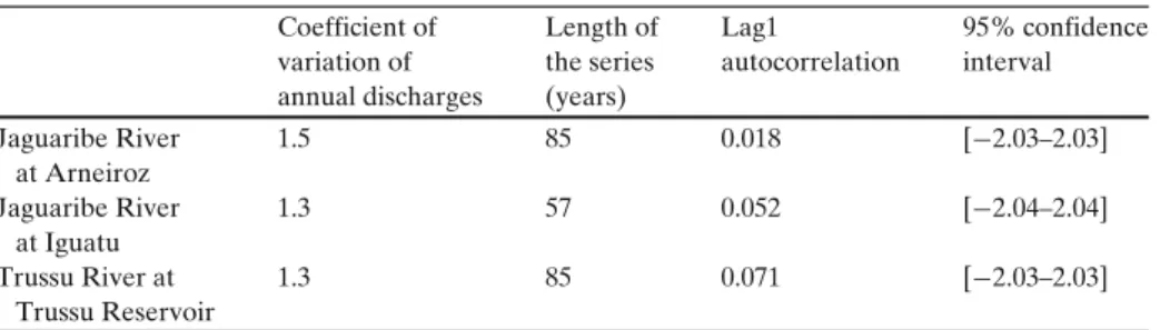
To prove the hypothesis of serial independence of annual discharges empirically, we analyzed two sections on the Jaguaribe River and one section on the Trussu River. The data were obtained from the Jaguaribe Water Management Plan. The results showed that the statistical hypotheses of no serial correlation are accepted in all cases (Table1).
6.2 RTD Application to Trussu Reservoir
The RTD can be used as a tool to model the transformations in the storage process as well as for preliminary reservoir sizing. A hydrological study using RTD can be performed in six steps: (1) evaluating the river hydrological regime by the mean and coefficient of variation of annual inflows from historical records or regionalization; (2) computing the reservoir dimensionless shape factor using Eq.3; (3) computing the dimensionless evaporation factor according to fE=(3α1/3.E/1/3)/μ1/3; (4) com-puting the dimensionless capacity factor fK = K/μ; (5) selecting the diagram that
Table 1 Serial independence tests on the Jaguaribe river basin, Ceará State, Brazil
Coefficient of Length of Lag1 95% confidence variation of the series autocorrelation interval annual discharges (years)
Jaguaribe River 1.5 85 0.018 [−2.03–2.03]
at Arneiroz
Jaguaribe River 1.3 57 0.052 [−2.04–2.04]
at Iguatu
Trussu River at 1.3 85 0.071 [−2.03–2.03]
Trussu Reservoir
Fig. 3 Annual hydrograph of Trussu river at Trussu reservoir, in Jaguaribe Valley, Ceará, Brazil
corresponds to theCvvalue; and (6) from the intersection of fKand fEisolines find, as shown in Fig.2, the evaporation, spill and release as a percent of the mean annual inflow.
The RTD was applied to the Trussu reservoir in the Jaguaribe River Basin, Ceará State in Northeast Brazil. The reservoir monthly inflows hydrograph is shown in Fig.3.
The reservoir data include storage capacity K=263.00 hm3
; mean annual inflow µ = 72.74 hm3; the coefficient of variation of annual inflows Cv = 1.3; and the maximum water depth hMAX =34.5 m. The monthly evaporation data are shown
in Table2. The net precipitation over the lake in the dry season (precipitation minus evaporation) and the seepage are negligible.
Additionally, as an academic evaluation, we use the same reservoir data, except we assume that the Cv values is 0.6. The results demonstrate the importance of the Cv values on the water budget for high evaporation conditions.
To solve this problem, the first step is to divide the year into two seasons. From the annual hydrograph of inflows, the dry season was defined as the period from June to December. The estimated values of the RTD dimensionless parameters fKand fE
are determined. The dry season evaporation is equal to 1.11 m (sum of evaporation depths from June to December).
Table 2 Mean evaporation depth in the Trussu reservoir in the Jaguaribe river basin in Ceará State (mm)
Jan Feb Mar Apr May Jun Jul Aug Sep Oct Nov Dec
The RTD parameters are: Dimensionless capacity factor
fK=K
μ=263.0∗106
73.74∗106=3.5
Dimensionless reservoir shape factor
α=K
(hM AX)3=263∗106
(34.5)3=6405
Dimensionless evaporation factor
fE=
3α1/3E
μ1/3=
3∗64051/3∗1.1
263∗1061/3
=0.15
Using the RTD forCV equal to 1.3 and obtaining the intersection of the isolines fE
(0.15) and fK(3.5) as shown, we determine that Mean release=50%; Mean spill=
27%; Mean evaporated volume=23% in terms of the mean annual inflow. Thus,
E{D} =0.50µ=0.50×73.74=36.87hm3/year;
E{EV} =0.23µ=0.23×73.74=16.96hm3/year;
E{SP} =0.27µ=0.27×73.74=19.91hm3/year;
The yield is Y=E{D} / 0.95=38.81 hm3 /year.
For Cv equal to 0.6 the following values were obtained: mean release = 80%; Mean spill =6%; Mean evaporated volume = 14% in terms of the mean annual inflow. Thus,
E{D} =0.80µ=0.80×73.74=58.99hm3/year;
E{EV} =0.14µ=0.14×73.74=10.32hm3/year;
E{SP} =0.06µ=0.06×73.74=4.42hm3/year;
The yield is Y=E{D} / 0.95=62.09 hm3 /year.
These results show the effects of inflow variability in the semi-arid region. The releases increase by 60%; the evaporations loss decreases by 39%; and the spills decrease by 78%. These results show the importance of inflow variability in the storage process, especially in high evaporation regions. The water is kept in the reservoir for a longer period of time, and the opportunity for evaporation increases.
Table 3 Trade-off release-evaporation-spill in the Trussu reservoir obtained from the regulation triangle diagram
Dimensionless capacity Release (%) Evaporation (%) Spill (%)
Cv=1.3 Cv=0.6 Cv=1.3 Cv=0.6 Cv=1.3 Cv=0.6
3.5 50 80 23 14 27 6
3.0 47 79 20 13 33 8
2.5 44 77 18 11 38 12
2.0 40 73 16 10 44 17
1.5 35 66 13 9 52 25
Fig. 4 aApplication of the Regulation Triangle Diagram Cv=1.3 for Trussu Reservoir at Jaguaribe River Basin in Northeast of Brazil. The results show the transformation of the mean annual inflow in release, evaporation and spill for several reservoir capacities.bThe hypothetical case of Trussu with Cv=0.6
To analyze the trade-off spill–release–evaporation, one can follow the isoline fE=
0,15 and obtain the values for the other dimensionless capacities (e.g., fK=3.0, 2.5, 2.0, 1.5 and 1.0). The results are shown in Table3and Fig.4(a, b).
It can be observed that for Cv = 0.6, the release from a reservoir with fK =
1.0 (55%) is greater than the release from a reservoir with fK = 3.5 in a region
where Cv= 1.3 (50%). These values indicate why reservoirs are built with high dimensionless capacities in semi-arid regions, where fKis typically greater than two.
7 Key Point: Yield Estimation from Monthly and Yearly Data
It is critical in the TRD model to divide the year into two seasons to estimate the dimensionless evaporation factor. That point was studied by Cavalcante Filho (2007) who evaluated 50 reservoirs in Ceará State. He found the length of the dry season that makes the yield estimated from the RTD equal to the yield computed using monthly data. He found values of the dry season length that range from six to 7 months for Ceará State that give a good approximation
8 Summary and Conclusions
This article describes a graphical procedure for modeling the yield–evaporation spill for water-supply reservoir planning: the Regulation Triangle Diagram (RTD). There are two points to be considered in the RTD method: (1) the diagram itself, which depicts the expected steady-state allocation of reservoir outflows among three mutually exclusive pathways, the release, spill and evaporation; (2) and the construction of diagrams for a given regional hydrological regime.
Considering the second point, a set of diagrams can be built to determine the parameters of a given region with similar hydrological characteristics. The diagram range was made to encompass the conditions of Brazil’s semi-arid climate with a coefficient of variation ranging from 0.6 to 1.6 and intermittent rivers.
Notation
At Lake area at beginning of year t Atw Lake area end of wet season on year t
Cv Coefficient of variation of reservoir annual inflows Dt Release from the reservoir during year t
E Evaporation depth from the reservoir at dry season EDA Extended deficit analysis
fE Reservoir dimensionless evaporation factor
fK Reservoir dimensionless capacity
fM Reservoir dimensionless yield
It Reservoir annual inflow at year t K Reservoir capacity
N Number of years on reservoir simulation NF Number of failure years on reservoir simulation
NNF Number of no failure years on reservoir simulation
qt Ratio between the release in the year t and the reservoir yield
R Reservoir reliability RTD Regulation triangle diagram SPA Sequent peak algorithm
SPt Volume spilled from the reservoir during year t
S-Y-R Storage yield reliability TPM Transition probability matrix Y Reservoir yield
Zact Reservoir activity capacity
Zt Reservoir storage contents at beginning of year t
Zt+1w Reservoir storage contents at end of wet season on year t
Ztd Reservoir storage contents at end of dry season on year t
Ztw Reservoir storage contents at end of wet season on year t
µ Mean annual inflow into the reservoir in volume units ϕ Expected value of qt
Acknowledgements This paper is a result of significant research in reservoir sizing supported by CAPES, CNPq, FINEP and FUNCAP in Brazil. Prof. Renata Luna and Dr. João Fernando Menescal were very helpful in the diagram design. The comments of the editor and reviewers are gratefully acknowledged.
Appendix: RTDs for Cv=0.6 to 1.6
References
Campos JNB (1987) A procedure for reservoir sizing on intermittent rivers under high evaporation rate. PhD Diss. Colorado State University, Fort Collins, Co, USA
Campos JNB (1991) Dimensionamento de reservatórios: O Método do Diagrama Triangular de Regularização. UFC, Fortaleza, Ce, Brazil
Campos JNB, Nascimento LSV, Studart TMC, Barcelos DG (2004) Desvios nas estimativas de vazões regularizadas resultantes da representação das relações cota x área x volume por equações matemáticas In: Proc of XXI Congresso Latino Americano de Hidráulica held in São Pedro. São Paulo, Brazil; International Association of Hydraulic Resources
Cavalcante Filho EC (2007) Regularização de vazões em reservatórios através de modelos mensal e bi-sazonal. MSc Thesis, Universidade Federal do Ceará, Fortaleza, Ce Brazil
Ceará State Water Law (1994) State Decree n0 23067/94
Celeste AB, Bilib M (2009) The role of spill and evaporation in reservoir optimization models. Water Resour Manag 24:617–628. doi:10.1007/s11269-009-9468-4
COGERH/ENGESOFT (2000) Plano de Gerenciamento das Águas da Bacia do Rio Jaguaribe. Fortaleza, Ceará
Hazen A (1914) Applied stochastic theory of storage in evolution. In: Chow VT (ed), Advances in hydrosciences, vol 12. Academic, NY
Klemes V (1981) Storage to be provided in impounding reservoirs for municipal water supply. Trans Am Soc Civ Eng 77:1539–640
Montaseri M (2000) Sthocastic investigation of the planning charactheristics of within-the-year and over-year reservoir system. PhD thesis. Departament of Civil And Offshore Engineering. Heriot-Watt University Edinburg, UK
Montaseri M, Adeloye AJ (2004) A graphical rule for volumetric evaporation loss correction in reservoir capacity-yield planning in Urmia Region, Iran. Water Resour Manag 18:55–74 Moran PAP (1954) A probability theory of dams and storage system. Aust J Appl Sci 5:116–126 McMahon TA, Adeloye AJ (2005) Water resources yield. Water Resources Publications, Colorado.
LLC; 2005
McMahon TA, Mein RG (1986) River and reservoir yield. Water Resources Publications. Fort Collins, Co
McMahon TA, Pegram GG, Vogel RM, Peel MC (2007a) Revisiting reservoir storage-yield using a global streamflow database. Adv Water Resour 30:1858–1872
McMahon TA, Pegram GG, Vogel RM, Peel MC (2007b) Review of Gould Dincer reservoir storage yield estimates. Adv Water Resour 30:1873–1882
Opricovic S (2009) A compromise solution on water resources planning. Water Resour Manag 23:1549–1561. doi:10.1007/s11269-008-9340-y
Rippl W (1883) Capacity of storage reservoirs for water supply. Minutes Proc Inst Civ Eng 71: 270–278