Phytoplankton response to nutrient pulses in an upwelling region: microcosms experiments

UNIVERSIDADE DE LISBOA

FACULDADE DE CIÊNCIAS

DEPARTAMENTO DE BIOLOGIA ANIMAL

Phytoplankton response to nutrient pulses in an upwelling

region: microcosms experiments

Afonso Miguel Barros Barreto Ferreira

Mestrado em Ecologia Marinha

Dissertação orientada por:

Doutora Ana C. Brito

I

“Afortunadamente, el contacto con la Naturaleza hace ver continuamente la limitación de nuestros esquemas y lo poco que sabemos.”

I

ACKNOWLEDGEMENTS

Em primeiro lugar, gostaria de agradecer à Doutora Ana C. Brito. Por todo o apoio, por toda a motivação e por toda a paciência que teve durante a orientação da tese. Obrigado também por ser um exemplo como investigadora e por estar sempre disponível para me ajudar.

Não poderia deixar também de destacar e agradecer às seguintes pessoas pelo papel fundamental que tiveram na realização deste trabalho: Carolina Sá, Nelson Silva, Ana Margarida Dias e Carolina Beltrán. Obrigado também pela disponibilidade para tirar dúvidas e pela grande ajuda nesta fase final. Gostaria ainda de agradecer a todas as pessoas que ajudaram no trabalho de laboratório, seja cá ou no Chile, em especial aos seguintes: Ana Amorim, Paola Reinoso, Randy Finke, Ricardo Calderón, Ricardo Prego, Sylvain Faugeron, Vanda Brotas, Vera Veloso e Wiebe Kooistra.

À Professora Isabel Domingos, pelo encorajamento e por procurar sempre defender os alunos do seu mestrado.

A todos os meus amigos que acompanharam durante este processo. Desde o pessoal da Madeira, aos amigos da licenciatura e mestrado (tanto de Ecologia Marinha como de Ecologia e Gestão Ambiental). Sem vocês, teria sido bem mais complicado manter a minha sanidade mental ao longo deste ano. Por fim, um obrigado especial à Rita e à minha família, em especial aos meus pais e à Teresa.

II

The work hereby presented has been submitted to an international journal as follows:

Ferreira, A.M., Sá, C., Silva, N., Beltrán, C., Dias, A.M., Brito, A.C., submitted. Phytoplankton response to nutrient pulses in an upwelling region: microcosms experiments. Journal of Experimental Marine Biology and Ecology.

III

ABSTRACT

The occurrence of nutrient enrichment in coastal areas can, in severe cases, lead to serious disturbances in marine ecosystems. Much is still to be done to understand how phytoplankton communities respond to natural and anthropogenic enrichment. This knowledge is essential to evaluate the implications on ecosystem functioning. The main goal of this study is to understand the response of phytoplankton communities to pulse nutrient enrichments in a region of intense upwelling conditions, namely the Humboldt Current System. In order to achieve this, a microcosm experiment with natural assemblages was conducted. In this experiment, two different experimental treatments were established to achieve N or P-limitation in the microcosms. The microcosms were enriched at the beginning and at half the duration of the experiment. Laboratory work included the analysis of nutrients, as well as phytoplankton pigments (HPLC) and cell abundances (microscopy). The phytoplankton community structure was also evaluated using chemotaxonomy (HPLC-CHEMTAX). Post-bloom conditions were observed at the beginning of the experiment, characterized by high content of chlorophyll a degradation products. A fast response to the initial enrichment was observed in both treatments as biomass increased from day 0 to 1. After the second enrichment pulse, a new biomass increase was observed as cell abundances peaked on Day 4. However, abundances slightly dropped in the remainder of the experiment. Although higher biomass values were found under higher DIN concentrations, the community’s composition was similar in both experimental treatments. Centric diatoms, especially Chaetoceros sp., dominated samples in both enrichments, suggesting growth advantages. Phytoflagellates and pennate diatoms were also common, while abundances of dinoflagellates, on the other hand, were low. HPLC-CHEMTAX results were not in agreement with the ones obtained from cell counts, possibly due to changes in the cells’ pigment content. These studies are relevant for understanding the functioning of phytoplankton communities and its influence on the whole ecosystem dynamics, thus being helpful for environmental quality assessment and management of marine resources.

Keywords: Phytoplankton Assemblage, Microcosm Experiments, Nutrient enrichment,

IV

RESUMO ALARGADO

O enriquecimento em nutrientes de zonas costeiras pode advir de diferentes fontes, podendo causar graves distúrbios nos ecossistemas marinhos. Este enriquecimento em nutrientes pode levar a que ocorra eutrofização, podendo esta ser classificada como antropogénica ou natural, consoante a origem do enriquecimento. Nos casos de origem antropogénica, esta pode ocorrer, por exemplo, devido à escorrência de compostos químicos provenientes de atividades humanas ou devido à deposição atmosférica de gases. Já nos casos em que a origem apresenta um caráter natural, as causas mais comuns são o transporte fluvial de nutrientes, quando não influenciado pelo Homem, ou o afloramento costeiro (upwelling). Este último é particularmente importante nos quatro sistemas de afloramento costeiro de fronteira oriental: a Corrente da Califórnia, a Corrente das Canárias, a Corrente de Benguela e a Corrente de Humboldt. Estes sistemas, apesar de ocuparem apenas 2% do oceano, contribuem para mais de 20% do total de peixe capturado a nível global. O Sistema da Corrente de Humboldt, que se estende desde cerca dos 42ºS até ao equador e engloba a costa do Equador, Perú e parte da costa do Chile, distingue-se dos restantes pela sua elevada produtividade pesqueira. O enriquecimento em nutrientes proveniente do afloramento costeiro é extremamente importante para as comunidades marinhas locais, principalmente para os produtores primários. O fitoplâncton, como componente basal das teias tróficas marinhas, tem um papel muito importante para o funcionamento do ecossistema. Como tal, qualquer alteração ambiental que afete as comunidades fitoplanctónicas, seja na turbulência da coluna de água ou na disponibilidade de luz ou em nutrientes, poderá ter consequências nos restantes elementos da teia trófica. Deste modo, é de extrema importância compreender-se como as comunidades de fitoplâncton respondem a enriquecimentos em nutrientes, quer estes sejam de origem natural ou antropogénica. Este conhecimento é essencial para se conseguir avaliar os potenciais impactos de alterações ambientais no funcionamento do ecossistema. Uma das melhores ferramentas disponíveis para se avaliar a dinâmica do fitoplâncton e a sua relação com enriquecimentos em nutrientes é a realização de experiências laboratoriais com comunidades naturais.

Deste modo, o principal objetivo deste trabalho é compreender a resposta de uma comunidade de fitoplâncton ao enriquecimento em nutrientes numa região com elevada intensidade de upwelling. De forma a atingir este objetivo, foram estabelecidas diversas metas específicas: i) avaliar a resposta a nível da biomassa a eventos de enriquecimento em nutrientes previamente estipulados; ii) estudar a sucessão da comunidade durante e após o enriquecimento; iii) averiguar se a comunidade reage de forma diferente a eventos discretos de enriquecimento em nutrientes com composições distintas; iv) analisar se o uso complementar de uma abordagem quimiotaxonómica (HPLC-CHEMTAX) pode fornecer informações adicionais de elevada relevância.

De forma a cumprir estes objetivos, foi realizada uma experiência com recurso a microcosmos que durou seis dias. A recolha de água para a experiência foi efetuada junto à baía de Algarrobo, na zona central do Chile (30-40ºS). Foram estabelecidos dois tratamentos experimentais: o tratamento N-limited (limitado em azoto) e o tratamento P-N-limited (limitado em fósforo). Nestes tratamentos, o objetivo era submeter a comunidade de fitoplâncton a condições de limitação em azoto ou fosfato, consoante o tratamento, de acordo com o rácio de Redfield (N-limited = N:P < 16:1; P-limited = N:P >16:1). Para tal, os microcosmos foram enriquecidos com uma solução que continha nitrato (NO3-),

fosfato (PO43−) e ácido silícico (Si[OH]4). A concentração de nitrato e fosfato adicionada aos

microcosmos foi ajustada de acordo com cada tratamento. O conteúdo em nutrientes, nomeadamente em azoto inorgânico dissolvido (DIN) e fosfato, foi analisado ao longo da experiência. A comunidade

V

fitoplanctónica foi também estudada através de contagens de células por microscopia e da análise dos pigmentos fotossintéticos via cromatografia liquida de alto desempenho (HPLC). Por fim, os resultados provenientes da HPLC foram utilizados para, através do programa de químiotaxonomia CHEMTAX v1.95, estimar a biomassa relativa dos principais grupos de fitoplâncton existentes nos microcosmos.

Analisando dados ambientais das duas semanas anteriores à experiência para a costa do Chile, os baixos valores da temperatura da superfície da água do mar e a existência de ventos perpendiculares de média intensidade junto à costa apontam para a existência de condições favoráveis à ocorrência de afloramento costeiro. Os valores de clorofila a observados (>1 mg m-3_{) parecem corroborar esta}

condição, principalmente nas semanas antes da experiência. A elevada concentração de pigmentos associados à degradação da clorofila a encontrada nos microcosmos aponta na mesma direção e sugere que a comunidade de fitoplâncton estudada estava num estado pós-florescência (bloom).

A comunidade respondeu de forma rápida ao enriquecimento inicial, aumentando a sua biomassa logo no primeiro dia da experiência. Este aumento foi observado tanto para a clorofila a como para a abundância de células em ambos os tratamentos. Devido ao crescimento do fitoplâncton, houve um grande consumo dos nutrientes, principalmente de DIN. Ao segundo e terceiro dia houve um declínio da abundância de fitoplâncton no tratamento N-limited, enquanto tal não se verificou no tratamento P-limited, onde se verificou inclusive um máximo no terceiro dia. Esta diferença pode estar relacionada com a disponibilidade de nutrientes nos microcosmos, i.e., a concentração de DIN no tratamento N-limited pode não ter sido o suficiente para promover o crescimento do fitoplâncton. Relativamente à comunidade fitoplanctónica, o principal grupo a ser beneficiado foi o das diatomáceas, em especial as diatomáceas cêntricas. Na verdade, observou-se um domínio de células de diatomáceas. Este domínio é algo recorrente em sucessões de upwelling e pode ser explicado pelas vantagens que este grupo apresenta no que diz respeito à assimilação de grandes concentrações de nutrientes e pela falta de predadores. O género Chaetoceros, em particular, devido ao seu domínio ao nível das abundâncias, mostrou ser uma componente bastante relevante para o funcionamento do ecossistema e a sua dinâmica deve ser tida em conta na gestão dos recursos marinhos desta região. Outro grupo comum nas amostras foi o dos fitoflagelados, principalmente das classes Chrysophyceae e Cryptophyceae. Por outro lado, as contagens de dinoflagelados foram relativamente baixas. Em relação ao segundo enriquecimento, houve um novo aumento das abundâncias de fitoplâncton em ambos os tratamentos. No entanto, após atingirem um máximo no quarto dia da experiência, as abundâncias sofreram um declínio. Tendo em conta que ainda parecia haver concentrações de nutrientes suficientes para o crescimento, especula-se que o crescimento da comunidade poderá ter sido limitado por um micronutriente (e.g. Fe), sendo que já foi reportado limitação em Fe para o sistema de afloramento costeiro de Humboldt. O segundo enriquecimento não pareceu ter tido um impacto significativo na estrutura da comunidade, uma vez que as abundâncias relativas dos principais grupos se mantiveram similares ao que tinha sido observado após o enriquecimento inicial. No geral, concluiu-se que, as comunidades de fitoplâncton estudadas reagiram de forma semelhante a enriquecimentos em nutrientes com composições distintas, embora as abundâncias observadas tenham sido mais elevadas no tratamento P-limited.

No entanto, a análise dos pigmentos fitoplanctónicos, incluindo o software CHEMTAX, revelou resultados contraditórios. Nestes, houve uma queda abrupta dos principais pigmentos fotossintéticos encontrados na amostra, como clorofila a ou a fucoxantina, a partir do segundo dia da experiência. Pensa-se que tal poderá ter acontecido devido à ocorrência de fotoaclimação, ou seja, as células terão otimizado a sua absorção de fotões, através da diminuição da concentração de clorofila a e de outros pigmentos fotossintéticos, de forma a evitar que a elevada luz incidente levasse a danos irreversíveis nos seus fotossistemas. Embora os microcosmos estivessem protegidos de radiação solar direta, é possível que esta proteção não tenha sido suficiente, levando então à fotoaclimação. Uma

VI

forma de evitar que isto aconteça em estudo futuros seria, por exemplo, aumentar a proteção solar. Os resultados deste estudo são relevantes para perceber o funcionamento das comunidades de fitoplâncton e os seus efeitos na dinâmica do ecossistema, podendo ser úteis para a avaliação de qualidade ambiental e gestão de recursos em habitats aquáticos. Para além disto, esta informação pode ser também utilizada na gestão de problemas relacionados com descargas de nutrientes nesta região, podendo servir de base para análises nos restantes sistemas de afloramento costeiro de fronteira oriental. Este conjunto de sistemas de upwelling, apesar das suas diferenças, já estudadas, na disponibilidade de nutrientes, na produtividade primária e nas próprias características do afloramento costeiro, sabe-se que têm em comum a predominância de comunidades de diatomáceas e condições de limitação em azoto semelhantes. Como tal, as respostas da comunidade de fitoplâncton considerada neste estudo podem ser similares às observadas nestes sistemas de afloramento costeiro, particularmente nos casos em que posso ocorrer limitação em ferro, como o sistema de afloramento costeiro da Corrente da Califórnia.

VII

TABLE OF CONTENTS

ACKNOWLEDGEMENTS ... I

ABSTRACT ... III

RESUMO ALARGADO ... IV

TABLE OF CONTENTS ... VII

LIST OF TABLES ... VIII

LIST OF FIGURES ... IX

LIST OF ABBREVIATIONS AND SYMBOLS... XIII

1.

INTRODUCTION ... 1

1.1. State of the art ... 1

1.2. Aim and objectives ... 6

2.

METHODS ... 7

2.1. Study site ... 7

2.2. Seawater sample collection ... 8

2.3. Experimental design ... 8

2.4. Nutrient Analysis ... 10

2.5. Phytoplankton community analysis ... 10

2.5.1. Cell abundances analysis ... 10

2.5.2. HPLC analysis ... 10

2.5.3. CHEMTAX Analysis ... 11

3.

RESULTS ... 12

3.1. Pre-experiment environmental conditions ... 12

3.2. Chlorophyll and nutrients dynamics ... 14

3.3. Nitrogen-to-phosphorus ratio ... 16

3.4. Phytoplankton Community ... 17

4.

DISCUSSION ... 27

4.1. Post-bloom phytoplankton response to nutrient enrichment ... 27

4.2. Phytoplankton response to nutrient enrichment: Additional pulses ... 29

4.3. Chaetoceros dominance ... 30

4.4. Changes in pigment and photoacclimation ... 31

4.5. Final considerations ... 33

VIII

LIST OF TABLES

Table 2.1: Stock solution composition for each experimental treatment. ... 9

Table 2.2: Measured and target (in brackets) concentrations for DIN (dissolved inorganic

nitrogen) and phosphate on Day 0. ... 9

Table 2.3: Detected phytoplankton pigments concentrations throughout the experiment (mean

and minimum-maximum values) ... 10

Table 2.4: Initial and final pigments-to-chl a ratio matrices in CHEMTAX analysis. ... 11

Table 3.1: Cell abundances (mean and minimum-maximum values) of the 10 most abundant

taxa observed. ... 19

IX

LIST OF FIGURES

Figure 1.1: SNPP VIIRS mean sea surface temperature (SST) for 2015. The rectangles signal

the location of the four Eastern Boundary Upwelling Systems (EBUS). ... 2

Figure 1.2: Relationship between the nitrate uptake pathway (highlighted by the green dotted

line) and photosynthesis during periods of low temperature and high nitrate concentration.

Nitrate reductase (NR); Nitrite reductase (NiR); Dissolved organic nitrogen (DON); light

energy (hv); PSII (photosystem II), e- (electrons), RUBISCO (Ribulose-1,5-bisphosphate

carboxylase/oxygenase); PGA (phosphoglyceric acid). Adapted from Lomas and Glibert

(1999a). a). ... 4

Figure 1.3: A) Succession of phytoplankton communities as nutrients and turbulence decrease

(Mandala; Margalef, 1978). B) Succession of phytoplankton communities as nutrients and

turbulence decrease (main sequence) and alternative sequence that leads to red tide events,

showing main groups associated with each state (Margalef et al., 1979). C) Separation of

phytoplankton life-strategies (C, R and S) as a result of the interaction between nutrient

accessibility and light depth (Reynolds, 1987). ... 4

Figure 1.4: Revision of Margalef’s mandala, including 12 traits of marine phytoplankton. The

traits are: 1) the gradient of nitrogen forms preferentially assimilated, from ammonium to

nitrate and/or from organic to inorganic forms; 2) the gradient of the dissolved inorganic N/P

ratio; 3) the gradient of adaptation to high vs low light and autotrophy vs mixotrophy; 4) the

gradient of the cell’s motility, from absence of motility to swimming to strategies of vertical

sink/float migration; 5) the gradient of turbulence from low to high; 6) the gradient of

pigmentation of cells, through the relative proportion of pigments classes; 7) the gradient of

temperature from high to low; 8) the gradient of cell size, from small to large; 9) the gradient

of the phytoplanktont’s growth rate, from low to high; 10) the gradient of the tendency of

cells to be toxic or to produce other bioreactive compounds, from high to low; 11) the

ecological strategy gradient, ranging from r to K and 12) propensity for the resulting

production to constitute regenerated production or new production (Glibert, 2016). ... 5

Figure 2.1: The Humboldt Current System (HCS), with special emphasis on the Central Chile

region (30º-40ºS). Main upwelling centres are represented by black dots, while grey dots

represent sites with frequent upwelling. Coastal areas with occasional upwelling are shown as

dark lines. Adapted from Thiel et al., 2007. ... 7

Figure 2.2: Location (red triangle) of the seawater sample collection off Algarrobo Bay,

Chile. ... 8

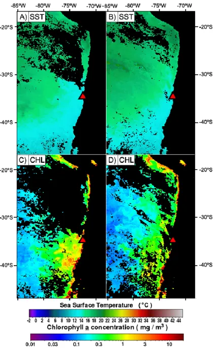
Figure 3.1: SNPP VIIRS mean sea surface temperature (SST; ºC) and chlorophyll a

concentration (CHL; mg m

) in the Chilean coast on the weeks preceding the experiment (on

the left: 9

-16

, on the right: 16

-23

of October 2013). The red triangle marks the location

of the water collection station. ... 12

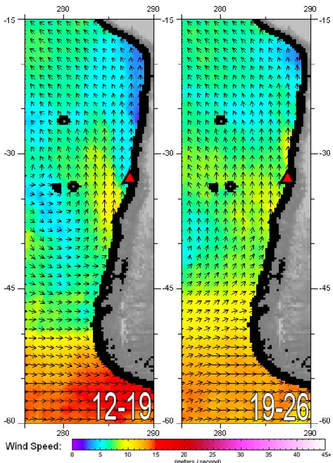
Figure 3.2: Mean WindSat wind vector direction and speed (ms

_{) in the South-East Pacific on}

X

the weeks preceding the experiment (12

_-19

_{and 19}

_-26

_{of October 2013). The red triangle}

marks the location of the water collection station. Note that the three round black patches on

the left side of the images correspond to the Desventuradas and Juan Fernández

archipelagoes. ... 13

Figure 3.3: Mean chlorophyll a concentrations (mg.m

) from Day 0 to Day 6 for both

treatments and control. Error bars shown are standard errors (SE). Note that the dotted,

dashed and solid lines respectively correspond to Control, N-limited and P-limited values. .. 14

Figure 3.4: Dissolved inorganic nitrogen (NO

+ NO

) mean concentrations (µM) from Day

0 to Day 6 for both treatments and control. Error bars shown are standard errors (SE). Note

that the dotted, dashed and solid lines respectively correspond to Control, N-limited and

P-limited values. ... 15

Figure 3.5: Phosphate (PO

) mean concentrations (µM) from Day 0 to Day 6 for both

treatments and control. Error bars shown are standard errors (SE). Note that the dotted,

dashed and solid lines respectively correspond to Control, N-limited and P-limited values. .. 15

Figure 3.6: Mean nitrogen-to-phosphorus ratio (N:P) from Day 0 to Day 6 for both treatments

and control. Error bars shown are standard errors (SE). Note that the dotted, dashed and solid

lines respectively correspond to Control, N-limited and P-limited values. ... 16

Figure 3.7: Mean total cell abundances (cells L

) from Day 0 to Day 6 for both treatments

and control. Error bars shown are standard errors (SE). Note that the dotted, dashed and solid

lines respectively correspond to Control, N-limited and P-limited values. ... 17

Figure 3.8: Mean cell abundances (cells L

) of pennate diatoms (solid line with dark squares),

centric diatoms (solid line with white circles), phytoflagellates (Chrysophyceae +

Cryptophyceae + Prasinophyceae + Prymnesiophyceae + Euglenophyceae; dotted line with

white triangles) and dinoflagellates (dash-dotted line with white diamonds) in the Control

treatment. Error bars shown are standard errors (SE). ... 18

Figure 3.9: Mean cell abundances (cells L

) of pennate diatoms (solid line with dark squares),

centric diatoms (solid line with white circles), phytoflagellates (Chrysophyceae +

Cryptophyceae + Prasinophyceae + Prymnesiophyceae + Euglenophyceae; dotted line with

white triangles) and dinoflagellates (dash-dotted line with white diamonds) in the N-limited

treatment. Error bars shown are standard errors (SE). ... 18

Figure 3.10: Mean cell abundances (cells L

) of pennate diatoms (solid line with dark

squares), centric diatoms (solid line with white circles), phytoflagellates (Chrysophyceae +

Cryptophyceae + Prasinophyceae + Prymnesiophyceae + Euglenophyceae; dotted line with

white triangles) and dinoflagellates (dash-dotted line with white diamonds) in the P-limited

treatment. Error bars shown are standard errors (SE). ... 19

Figure 3.11: Mean cell abundances (cells L

) of Chaetoceros sp. (dash-dotted line with black

diamonds), Nitzschia sp. (solid line with white triangle), Gymnodinium sp. (dotted line with

black square) and Scrippsiella sp. (dashed line with white circle) in the N-limited treatment.

Error bars shown are standard errors (SE). ... 20

Figure 3.12: Mean cell abundances (cells L

) of Chaetoceros sp. (dash-dotted line with black

XI

diamonds), Nitzschia sp. (solid line with white triangle), Gymnodinium sp. (dotted line with

black square) and Scrippsiella sp. (dashed line with white circle) in the P-limited treatment.

Error bars shown are standard errors (SE). ... 21

Figure 3.13: Total chlorophyll a (TChl a; dashed line with black squares) and chlorophyll a

degradation products - chlorophyllide a (Chlide a; dotted line with white diamonds),

pheophytin a (Phe a; solid line with white circles) and pheophorbyde a (Pheide a; grey line

with grey triangles) mean concentrations (mg m

) from Day 0 to Day 6 in the Control

treatment. Error bars shown are standard errors (SE). Note that pheophorbyde a

concentrations are measured in the secondary axis (right, in gray). ... 22

Figure 3.14: Total chlorophyll a (TChl a; dashed line with black squares) and chlorophyll a

degradation products - chlorophyllide a (Chlide a; dotted line with white diamonds),

pheophytin a (Phe a; solid line with white circles) and pheophorbyde a (Pheide a; grey line

with grey triangles) mean concentrations (mg m

) from Day 0 to Day 6 in the N-limited

treatment. Error bars shown are standard errors (SE). Note that pheophorbyde a

concentrations are measured in the secondary axis (right, in gray). ... 22

Figure 3.15: Total chlorophyll a (TChl a; dashed line with black squares) and chlorophyll a

degradation products - chlorophyllide a (Chlide a; dotted line with white diamonds),

pheophytin a (Phe a; solid line with white circles) and pheophorbyde a (Pheide a; grey line

with grey triangles) mean concentrations (mg m

) from Day 0 to Day 6 in the P-limited

treatment. Error bars shown are standard errors (SE). Note that pheophorbyde a

concentrations are measured in the secondary axis (right, in gray). ... 23

Figure 3.16: Mean concentrations (mg m

_{) of MgDVP (solid line with white squares),}

chlorophyll c

(Chl c

; dotted line with white circles), fucoxanthin (Fuco; dashed line with

grey triangles), chlorophyll b (Chl b; dash-dotted line with white circles) and chlorophyll a

(Chl a; dotted line with black diamonds) from Day 0 to Day 6 in the N-limited treatment.

Error bars shown are standard errors (SE). ... 23

Figure 3.17: Mean concentrations (mg m

_{) of MgDVP (solid line with white squares),}

chlorophyll c

(Chl c

; dotted line with white circles), fucoxanthin (Fuco; dashed line with

grey triangles), chlorophyll b (Chl b; dash-dotted line with white circles) and chlorophyll a

(Chl a; dotted line with black diamonds) from Day 0 to Day 6 in the N-limited treatment.

Error bars shown are standard errors (SE). ... 24

Figure 3.18: Chlorophyll a concentrations (absolute contribution; mg m

_{), estimated through}

the CHEMTAX analysis, for Haptophyceae (Hapto), dinoflagellates (Dinof), Chrysophyceae

(Chryso) and diatoms from Day 0 to Day 6 in the N-limited treatment. Error bars shown are

standard errors (SE). ... 24

Figure 3.19: Chlorophyll a concentrations (absolute contribution; mg m

), estimated through

the CHEMTAX analysis, for Haptophyceae (Hapto), dinoflagellates (Dinof), Chrysophyceae

(Chryso) and diatoms from Day 0 to Day 6 in the P-limited treatment. Error bars shown are

standard errors (SE). ... 25

Figure 3.20: CHEMTAX chlorophyll a absolute concentrations (mg m

) obtained through

CHEMTAX for diatoms against diatoms abundances (cells L

) for both experimental

XII

treatments. ... 25

Figure 3.21: CHEMTAX chlorophyll a absolute concentrations (mg m

) obtained through

CHEMTAX for dinoflagellates against dinoflagellates abundances (cells L

) for both

experimental treatments. ... 26

Figure 3.22: CHEMTAX chlorophyll a absolute concentrations (mg m

) obtained through

CHEMTAX for diatoms against diatoms abundances (cells L

_{), only for Days 1 and 2, for}

both experimental treatments. ... 26

Figure 3.23: CHEMTAX chlorophyll a absolute concentrations (mg m

) obtained through

CHEMTAX for dinoflagellates against dinoflagellates abundances (cells L

), only for Days 1

and 2, for both experimental treatments. ... 27

XIII

LIST OF ABBREVIATIONS AND SYMBOLS

β,β – Car β,β -Carotene Chl a Chlorophyll a Chl b Chlorophyll b Chl c2 Chlorophyll c2 Chl c3 Chlorophyll c3 Chlide a Chlorophyllide a

DIN Dissolved Inorganic Nitrogen

EBUS Eastern Boundary Upwelling Systems

FAO Food and Agriculture Organization of the United Nations

Fuco Fucoxanthin

HCS Humboldt Current System

Hex-fuco 19’-Hexanoyloxyfucoxanthin

HPLC High Performance Liquid Chromatography

MgDVP Mg-2,4-divinylpheoporphyrin a5 monomethyl ester

N:P Nitrogen-to-Phosphorus Ratio

NH4+ _Ammonium

NO2- Nitrite

NO3- Nitrate

OSPAR Convention for the Protection of the Marine Environment of

the North-East Atlantic

Phe a Pheophytin a

Pheide a Pheophorbide a

PO43- Phosphate

PTFE Polytetrafluoroethylene

Si[OH]4 Silicic acid

SNPP VIIRS Suomi National Polar-Orbiting Partnership Visible Infrared

Imaging Radiometer Suite

SST Sea Surface Temperature

1

1. INTRODUCTION

1.1. State of the art

The occurrence of nutrient enrichment in coastal areas may have different sources and, in severe cases, can lead to serious disturbances in marine ecosystems (Smith et al., 1999). Eutrophication is frequently considered as potentially harmful for aquatic ecosystems and able to disrupt ecosystem services. However, for truly understanding eutrophication, it is crucial to separate the process from its causes and consequences (Nixon, 1995).

Eutrophication can occur naturally or due to anthropogenic forcing, but it is always driven by enrichment in nutrients (Ferreira et al., 2011). Human-induced or cultural eutrophication is commonly associated with land-originated inputs, originating from point (e.g. wastewater effluent, runoff from mines or aquacultures, waste disposal sites or animal feedlots) or non-point sources (e.g. atmospheric deposition or runoff from agriculture or urbanization; Carpenter et al., 1998). This enrichment in nutrients can prompt a significant increase in the biomass of primary producers, leading to a decrease in transparency and to an increase in organic matter sedimentation. In severe cases of eutrophication, this situation may deteriorate as high consumption of oxygen from both grazers and sediment aerobic bacteria leads to oxygen depletion and, consequently, to mass death of fish and macroinvertebrates (Ferreira et al., 2011).

When eutrophication initially began to be widely regarded as a problem circa 1960s (Nixon, 1995), scientists initially thought of it as a state. For instance, Rodhe (1969) created a classification system for determining eutrophication in lakes that considered its primary production. In this system, a lake with 350-700 g C m-2 _year-1 _{was classified as eutrophic (in a polluted sense). Over the past few}

decades, however, some authors have argued that eutrophication should be rather seen as a process (e.g. Ansari et al., 2011; Ferreira et al., 2011; Nixon, 1995). During this period, the definition of eutrophication has been intensively discussed. Nixon (1995), searching for an operational definition, defined it as “an increase in the rate of supply of organic matter to an ecosystem”. However, this definition was deemed as insufficient for water quality management and, after further discussion, more adequate definitions emerged. For instance, the OSPAR Eutrophication Strategy defines it as the “enrichment of water by nutrients causing an accelerated growth of algae and higher forms of plant life to produce an undesirable disturbance to the balance of organisms present in the water and to the quality of the water concerned, and therefore refers to the undesirable effects resulting from anthropogenic enrichment by nutrients (…)” (OSPAR Commission, 2010). This and other similar definitions have been imperative for the implementation of environmental legislation that tackles eutrophication, such as the Marine Strategy Framework Directive (Directive 2008/56/EC; e.g. Cabrita et al., 2015; Ferreira et al., 2011; Fleming-Lehtinen et al., 2015)

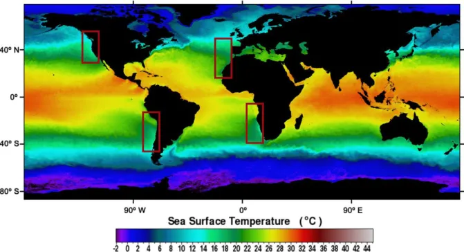
Natural eutrophication occurs due to natural processes, for example due to natural nutrient flow from rivers or upwelling. However, it should be noted that, nowadays, most rivers are highly influenced by anthropogenic action and that pristine rivers are scarce. In most cases, this sort of eutrophication is considered as an important part of the natural variability of a given aquatic system. Coastal upwelling occurs when deep nutrient-rich and cooler waters arise as winds drive alongshore, enhancing primary productivity (Thiel et al., 2007). This phenomenon is particularly important in four major coastal currents located in the eastern boundaries of the Pacific and Atlantic basins, the eastern boundary current systems (EBUS; Figure 1.1): the California Current System (CalCS), the Canary Current System (CanCS), the Humboldt Current System (HCS) and the Benguela Current System (BCS). Despite covering less than 2% of the ocean, these systems are responsible for 7% of the global marine primary production and more than 20% of global fish catches (Wang et al., 2015).

2

Notwithstanding their common upwelling occurrence, these systems are highly heterogeneous and there are differences in the timing, duration and intensity of the upwelling. For instance, in lower latitudes, upwelling can occur all year, while in higher latitudes it displays a seasonal pattern, occurring mainly during spring and summer (Wang et al., 2015).

Figure 1.1: SNPP VIIRS mean sea surface temperature (SST) for 2015. The rectangles signal the location of the four Eastern Boundary Upwelling Systems (EBUS).

The Humboldt Current System extends from ~42ºS up to the equator (Thiel et al., 2007) and encompasses the shoreline along Chile, Peru and Equador. Due to its heterogeneity, the HCS can be divided in three biomes: i) the upwelling system off Peru (~ 4-16ºS), known for its immense productivity and upwelling occurrence during all year, ii) the moderate to low productivity zone from southern Peru to northern Chile (18-26ºS) and iii) central Chile (30-40ºS), typical of seasonal upwelling and high productivity (Chavez and Messié, 2009). Despite displaying one the highest average primary productivities of all the EBUS (2.18 g C m-2 _day-1_{; Carr, 2002), its active area is}

smaller than BCS and CalCS, thus contributing to a lower annual primary productivity than its counterparts (Carr, 2002). Nonetheless, the HCS is one of the regions with highest fish production (representing 10% of the world fish catch; Chavez et al., 2008), particularly due to the well-known anchoveta (Engraulis ringens Jenyns, 1842) fishery off coastal Peru, whose landings from 2003-2012 averaged over 7 million tonnes (FAO, 2016). This production is due to the HCS’s unique efficiency in the energy transfer between trophic levels (Chavez and Messié, 2009), leading to a much higher fish per unit of primary production. Thus, as its main primary producers, phytoplankton communities have a major role in the maintaining the functioning of the HCS.

Marine phytoplankton communities can be very diverse, encompassing a myriad of life forms which may range from 0.2 µm to over 2 mm (Reynolds, 2006). For phytoplankton, apart from cell size (i.e. width), the surface-to-volume (S/V) ratio is also considered as a relevant trait for phytoplankton physiology. The higher the S/V ratio is, the easier it is for cells to assimilate nutrients and grow faster (Reynolds, 2006). The S/V ratio has direct implications on the constant of half saturation (KS, i.e. the

concentration of a given nutrient required to satisfy half of the maximum uptake capacity of the cell). Thus, smaller phytoplanktonts with high S/V ratios and low KS, such as cyanobacteria and small

3

flagellates (e.g. most Chrysophyceae, Cryptophyceae and Haptophyceae), can grow under lower nutrient conditions.

Photosynthesis is a process common to most primary producers in nature. In general, this process utilizes electromagnetic radiation as an energy source, carbon is fixed and oxygen is released. Photosynthesis is essential for the production of organic compounds (through the synthesis of organic carbon from inorganic carbon), converting light energy into chemical energy. Since photosynthesis cannot occur without light, phytoplankton is not able to grow under light limitation. However, living near the surface, where light intensity may be excessive, can result in photoinhibition and damage of cells’ photosystems. Thus, most phytoplanktonts generally live in an intermediate layer, called the deep chlorophyll maximum (DCM), where there exists an optimization of the utilization of light and nutrients. In fact, sustained phytoplankton growth is only possible if the concentration of nutrients in the surrounding waters is sufficient. For phytoplankton, the nutrients most often associated with growth limitation are nitrogen (N) and phosphorus (P), as both are essential for important internal components of the cell like nucleic acids (Reynolds, 2006). However, there are other elements that may act as limiting nutrients, such as iron (Fe), due to its important role as an electron acceptor in photosynthesis, and silicon (Si). Silicon, along with oxygen and hydrogen, makes up silicic acid (Si[OH]4), an important component for the skeleton (frustule) of diatoms. Thus, silicon limitation may

occur and inhibit diatom growth.

Nutrient requirements by phytoplankton have been extensively studied in the past. Redfield (1934, 1958) discovered that carbon, nitrate and phosphate concentrations observed in different oceans occurred in the same proportions (C:N:P = 106:16:1). He also concluded that the exact same proportions could be generally found in phytoplankton cells. This ratio, known as the Redfield ratio, is still used nowadays because of its importance for understanding ocean biogeochemistry. Later, the Redfield ratio was extended to include iron (C:N:P:Fe = 106:16:1:0.001; Sarmiento & Gruber, 2006) and silicon (C:Si:N:P = 106:15:16:1; Brzezinski, 1985) due to their role as possible limiting nutrients.

These nutrients can be available in both its inorganic or organic forms, but are generally assimilated by phytoplankton in its inorganic form. Inorganic nitrogen, for instance, is mainly available to phytoplankton in the form of the ions nitrate (NO3-), nitrite (NO2-) and ammonium (NH4+).

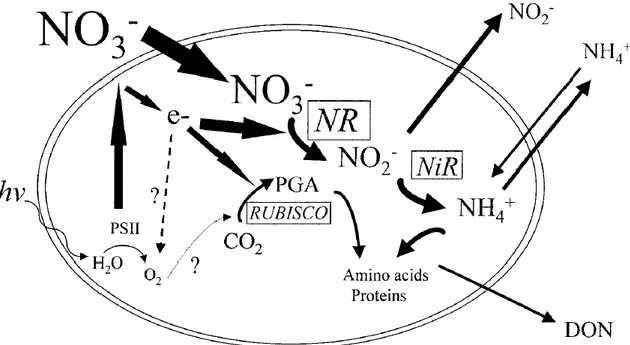
Of these three forms, nitrate is the most common in the open sea, hence being the one that is typically assimilated by phytoplanktonts (Reynolds, 2006). This status can change in coastal regions due to the influence of multiple inputs. Nonetheless, nitrate must be reduced to ammonium in order to be utilized intracellularly (Owens and Esaias, 1976; Figure 1.2). This process requires additional metabolic energy cost, which is why ammonium was, until recently, thought as the preferentially assimilated inorganic nitrogen compound for all phytoplankton groups (Dortch, 1990).

In spite of this theoretical disadvantage in assimilating nitrate, several studies have shown that diatom assemblages under low temperatures (<15ºC) and high concentrations of nitrate favour nitrate assimilation (Glibert et al., 2015; Lomas and Glibert, 1999a, b). Under such conditions, diatoms are highly productive and generate electrons in excess from photosynthesis. In order to avoid photoinibition of photosynthesis, cells have to dissipate some of these electrons through the reduction of nitrate (via nitrate reductase; see Figure 1.2). Thus, they hypothesized that nitrate assimilation is a strategy to maintain intracellular energy balance. This is particularly relevant for understanding the dynamics of diatoms in upwelling-influenced ecosystems given that low temperatures and high nitrate concentrations are typical of these regions.

4

Figure 1.2: Relationship between the nitrate uptake pathway and photosynthesis during periods of low temperature and high nitrate concentration. Nitrate reductase (NR); Nitrite reductase (NiR); Dissolved organic nitrogen (DON); light energy (hv); PSII (photosystem II), e- (electrons), RUBISCO (Ribulose-1,5-bisphosphate carboxylase/oxygenase); PGA (phosphoglyceric acid). Adapted from Lomas and Glibert (1999a). a).

Figure 1.3: A) Succession of phytoplankton communities as nutrients and turbulence decrease (Mandala; Margalef, 1978). B) Succession of phytoplankton communities as nutrients and turbulence decrease (main sequence) and alternative sequence that leads to red tide events, showing main groups associated with each state (Margalef et al., 1979). C) Separation of phytoplankton life-strategies (C, R and S) as a result of the interaction between nutrient accessibility and light depth (Reynolds, 1987).

5

However, it is not just light and nutrients that determine phytoplankton growth and ecology. Turbulence is also very important in shaping phytoplankton assemblages. In 1978, Margalef introduced his “mandala”, clarifying the underlying relation between turbulence and nutrient availability (Figure 1.3A). According to Margalef, turbulence, unless when excessive, could help the uptake of nutrients and assure the survival of non-motile populations, like most diatoms. In such an environment, motility would be regarded as a waste of energy. However, the less turbulent an environment is, the more essential motility becomes to avoid sinking and consequent cell losses, which is why dinoflagellates dominate stratified waters. The “mandala” successfully simplified this succession from r species (i.e. species that thrive under unstable environments, such as diatoms) to K species (i.e. typically associated with stable environments, such as dinoflagellates) in a typical temperate winter-spring bloom sequence. Later, Margalef tried to explain the formation of red tides as a divergence from the main succession promoted by nutrient inputs from terrestrial and anthropogenic sources (Margalef et al., 1979; Figure 1.3B).

Figure 1.4: Revision of Margalef’s mandala, including 12 traits of marine phytoplankton. The traits are: 1) the gradient of nitrogen forms preferentially assimilated, from ammonium to nitrate and/or from organic to inorganic forms; 2) the gradient of the dissolved inorganic N/P ratio; 3) the gradient of adaptation to high vs low light and autotrophy vs mixotrophy; 4) the gradient of the cell’s motility, from absence of motility to swimming to strategies of vertical sink/float migration; 5) the gradient of turbulence from low to high; 6) the gradient of pigmentation of cells, through the relative proportion of pigments classes; 7) the gradient of temperature from high to low; 8) the gradient of cell size, from small to large; 9) the gradient of the phytoplanktont’s growth rate, from low to high; 10) the gradient of the tendency of cells to be toxic or to produce other bioreactive compounds, from high to low; 11) the ecological strategy gradient, ranging from r to K and 12) propensity for the resulting production to constitute regenerated production or new production (Glibert, 2016).

6

The subject of phytoplankton life-strategies was again addressed by Reynolds in his “intaglio”, a conceptual model that divided phytoplanktonts in colonists (C-strategists), slow-growers (S-strategist) and ruderals (R-strategists) (Reynolds, 1987; Smayda and Reynolds, 2001; Figure 1.3C). This model differed from the Margalef’s mandala in some aspects: i) it originally focused on freshwater phytoplankton (although it has since been applied to marine waters, e.g. Alves-de-Souza et al., 2008; Brito et al., 2015); ii) each of the three adaptive strategy (C, S and R) may include r- or K-selected species and iii) it adapts the mandala’s nutrients and turbulence axes to nutrient accessibility and light/mixed depth, respectively. More recently, Margalef’s mandala was expanded by Glibert (2016), resulting in a highly complex updated mandala which covers twelve effects or response traits, such as the ecological strategy (r or K), temperature, cell size and relative availability of inorganic nitrogen or phosphorus (see Glibert, 2016 for more details; Figure 1.4). In this new mandala, diatoms are shown to be associated with, for example, high turbulence, low temperatures, higher concentrations of nitrate and nitrogen limitation. Another conclusion is that bloom-forming dinoflagellates are more associated with nitrogen limitation, low temperatures and higher growth rates than low biomass dinoflagellates. These models are crucial for understanding phytoplankton dynamics in an ever-changing world.

Changes in environmental conditions can lead to changes in phytoplankton communities. As seen above, light, nutrient availability and turbulence or stratification have implications on the phytoplanktonic groups that bloom and dominate an ecosystem. Since any given change in the community might have consequences for the ecosystem, particularly in the local trophic chain, the dominance of a particular phytoplankton group may determine which organisms top the trophic web. Cury (2008) demonstrated such dynamic in marine trophic webs off Cape Agulhas. On one hand, when turbulence is low, phytoflagellates dominate. These are then consumed by small copepods, which in turn are consumed by sardines. On the other hand, diatoms bloom when turbulence is high and are consumed by larger copepods. These larger copepods are preferentially consumed by anchovies. Thus, there is a natural oscillation between high biomasses of sardines or anchovies.

There is still much to learn about how phytoplankton communities react to nutrient enrichments, whether these enrichments are natural or anthropogenic. This knowledge would be essential for providing insight on their implications for the ecosystem functioning. Thus, solving this challenge would be the first step towards the possibility of assessing the potential impacts of changes in environmental conditions, namely nutrient availability. One crucial way is through laboratory experiments with natural phytoplankton assemblages. Despite its intrinsic limitations (Carpenter, 1996; Schindler, 1987), these experiments are one of the best tools available to understand phytoplankton dynamics and its relation with nutrients inputs (Domingues et al., 2015).

1.2. Aim and objectives

The main goal of this study is to understand the response of phytoplankton communities to pulse nutrient enrichments in a region of intense upwelling conditions. To achieve this goal, several specific objectives were established: i) assess the biomass response to known nutrient pulses; ii) study the succession of the phytoplankton community under enrichment; iii) examine if the phytoplankton community reacts differently to nutrient pulses with distinct compositions; iv) analyse if the complementary use of a chemotaxonomy approach (HPLC-CHEMTAX) can provide additional valuable insight.

7

2. METHODS

2.1.

Study site

The coastal waters off Central Chile (30-40ºS; Figure 2.1) are one of the main biomes of the Humboldt Current System. Upwelling in this region displays a seasonal recurrent pattern, occurring during the austral spring-summer (October-March), when favourable winds (from S/SW) predominate (Thiel et al., 2007). Due to the high spatial heterogeneity of the coastline, upwelling is more intense in the following locations: off Coquimbo (30ºS), off Valparaíso (33ºS) and off Concepción (36ºS). These upwelling centres contribute to a high productivity during upwelling season and are the major reason why Chile became one of the main “fishing nations”, with high abundance of sardines and anchovies’ stocks (Peterson et al., 1988). The mean upwelling intensity in Central Chile is high (~1.2 m2 _s-1_{), but}

is considerably lower than other intense upwelling regions (e.g. >2 m2 _s-1 _{off Peru and off Namibia;}

PFEL upwelling index, Wang et al., 2015). However, it is also much higher than what can be found off the Iberian Peninsula (<1 m2 _s-1_{; Wang et al., 2015), per example. During upwelling season,}

chlorophyll a ranges between 3.8-26 mg m-3_{, much higher values than what have been measured}

during winter (1-2.5 mg m-3_{; González et al. 1989; Montecino et al. 2004).}

Figure 2.1: The Humboldt Current System (HCS), with special emphasis on the Central Chile region (30º-40ºS). Main upwelling centres are represented by black dots, while grey dots represent sites with frequent upwelling. Coastal areas with occasional upwelling are shown as dark lines. Adapted from Thiel et al., 2007.

This region has relatively low average sea surface temperature (SST; e.g. 14ºC off Valparaíso; Hormazabal et al., 2001), mainly due to the Humboldt Current upward transport of nutrient-rich cooler subantartic waters and, in the austral summer, to strong upwelling. However, this dynamic can be interrupted during El Niño events. When these events occur, warm and nutrient-poor equatorial waters are conveyed to coastal Chile, interrupting the flow of the Humboldt Current. This leads to a general increase in SST and, consequently, a decrease in upwelling intensity in the region. Moreover, it can

8

cause negative impacts on the local communities (Thiel et al., 2007). One of the main characteristics of this region is the occurrence of iron limitation during intense upwelling events. This trait is common in the HCS, mostly due to its short continental shelf and low riverine influence, the main sources of iron in coastal waters (Hutchins et al., 2002; Thiel et al., 2007).

2.2.

Seawater sample collection

Seawater was collected on the 25th _{October of 2013, at noon, from a coastal point facing the Algarrobo}

Bay in the Valparaíso region, Chile (33°19'16.9"S 71°45'36.3"W; Figure 2.2). Niskin bottles were used to collect approximately 200 L of seawater from the surface (0-5 m depth). Seawater was then filtered through a 200μm mesh in order to remove zooplankton, macroalgae and detritus.

Figure 2.2: Location (red triangle) of the seawater sample collection off Algarrobo Bay, Chile.

The seawater was then rapidly transported in 50L jerricans to the laboratory in the Estación Costera de Investigaciones Marinas “Las Cruces” (ECIM; 33°30'05.8"S 71°38'01.7"W), where it was agitated to ensure homogenisation and partitioned into plastic containers, the microcosms/incubators used in these experiments. The containers were acid-washed and rinsed with natural seawater for 3 times to ensure that no contamination, particularly nutrients, was taking place. They were subsequently filled with 3 L and allowed to rest in a tank with regular light conditions until the following day.

2.3. Experimental design

In order to assess the response of the phytoplankton community to different nutrient enrichments, two different experimental treatments were established: the N-limited and the P-limited treatments. In each treatment, the microcosms were enriched with a solution containing nitrate (NO3-)

and phosphate (PO43−), specifically prepared to achieve those conditions, using the N:P Redfield ratio

as a benchmark (N-limited = N:P < 16:1; P-limited = N:P >16:1; Redfield, 1958). Both solutions also contained silicic acid (Si[OH]4) to prevent Si-limitation. These solutions were prepared with analytical

grade NaNO3,NaH2PO4 and Na2SiO3 reagents (Table 2.1), thus only altering the reactants’ ratio to

reach the adequate nutrient final concentrations. The recipes chosen for achieving each of these solutions followed previous works by Brito (2010), Brito et al., (2010) and Edwards et al. (2003,

9

2001). A control treatment was also established.

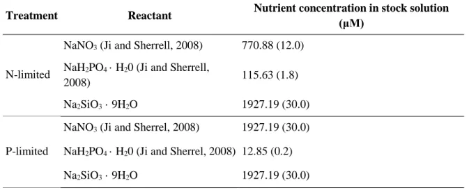
Table 2.1: Stock solution composition for each experimental treatment and target concentrations in the microcosms (in brackets)

Treatment Reactant Nutrient concentration in stock solution

(μM)

N-limited

NaNO3 (Ji and Sherrell, 2008) 770.88 (12.0)

NaH2PO4 · H20 (Ji and Sherrell,

2008) 115.63 (1.8)

Na2SiO3 · 9H2O 1927.19 (30.0)

P-limited

NaNO3 (Ji and Sherrel, 2008) 1927.19 (30.0)

NaH2PO4 · H20 (Ji and Sherrel, 2008) 12.85 (0.2)

Na2SiO3 · 9H2O 1927.19 (30.0)

The experiment started on the 26th _{of October 2013 (Day 0). Containers were manually}

agitated 4 times per day and temperature and salinity were monitored everyday with the help of a thermometer and a refractometer, respectively, to make sure these conditions remained stable throughout the experiments.

2.2.1. Experiment details

The experiment focused on phytoplankton response to pulse enrichment events, simulated in laboratory by two separate microcosm enrichments. These enrichments occurred at day 0 and at day 3, halfway through the experiment.

Table 2.2 displays the initial post-enrichment nutrients concentrations. 24 microcosms (12 per treatment) were subjected to both treatments considered previously: N-limited and P-limited. Another 12 containers were used as controls. From day 0 to day 6, two containers (plus one control) from each treatment were sacrificed every day. Sacrificed containers were used for the measurement of nutrients and phytoplankton pigments and for microscopic analysis of the phytoplankton community. This approach prevented any interference with the ongoing experiment, avoiding any contamination to the incubators. The enrichment was done by adding 47.6 mL of the solution associated with each treatment (Table 2.2). The added volume was the same for each treatment to avoid any issues related to dilution factors. The second enrichment pulse, on day 3, was intended to assess how the community reacted to an enrichment event shortly after the other. The experiment ended in day 6, when the last microcosms were removed.

Table 2.2: Measured and target (in brackets) concentrations for DIN (dissolved inorganic nitrogen) and phosphate on Day 0.

Treatment Nutrient concentration (μM) DIN Phosphate Control 0.8 1.0 N-limited 13.0 (12.0) 2.9 (1.8) P-limited 30.8 (30.0) 1.2 (0.2)

Note: Control’s nutrient concentrations correspond to the measured concentrations in natural seawater and therefore should be regarded as the surplus found regarding the targets concentrations.

10

2.4. Nutrient Analysis

A sample of 200 mL was collected from each sacrificed incubator, frozen immediately at – 25 ºC and subsequently analysed to measure dissolved inorganic nutrients (nitrate and nitrite (NO2-+NO3

-), phosphate (PO43-) and silicic acid (Si[OH]4) with the aid of a AutoAnalyzer, accordingly to the

methodology of Atlas et al. (1971). The analyses were carried out at the Pontificia Universidad Católica de Valparaíso. Nitrogen-to-phosphorus ratio (N:P) was calculated since it significantly influences the phytoplankton species composition (Tilman et al., 1982).

2.5. Phytoplankton community analysis

2.5.1. Cell abundances analysis

Samples (125 mL) were taken from the sacrificed containers and subsequently preserved with neutral Lugol’s solution (2%). Samples were then kept in brown-glass flasks and stored in a cool place. Before the analysis, 100 mL settling chambers were used for 48 hours after gently agitating the samples for homogenisation. Phytoplankton cells were counted and identified to the lowest taxon possible (Lund et al., 1958; Utermöhl, 1958) using an inverted light microscope, in agreement with the proceedings of Chrétiennot-Dinet (1990), Hoppenrath et al. (2009), Ricard (1987), Sournia (1986) and Tomas (1997).

2.5.2. HPLC analysis

300 mL samples were filtered with Whatman GF/F glass fibre filters (25 mm diameter and 0.7 µm pore size) in low light conditions. After filtration, filters were stored at -80ºC until analysis. In order to extract phytoplankton pigments, the filters were placed in centrifuge tubes for extraction in 3 mL of 95% cold-buffered methanol (2% ammonium acetate), containing the pigment trans-β-Apo-8’-carotenal (0,05 mg L-1 _{as the internal standard). Samples were then sonicated (Bransonic 1210) for 5}

minutes, placed in the freezer (-20 ºC) and allowed to rest for one hour. Following 5 min centrifugation at 3ºC, the extract was filtered through PTFE membrane filters (0.2 µm pore size) to ensure that no residues were inserted in the HPLC system. For pigment analyses, Zapata et al. (2000) method was carried out with a 1 ml min-1 _{flux and an injection volume of 100 µl. This method uses a}

monomeric C8 column and a mobile phase containing pyridine. After pigment identification from absorbance spectra and retention times, concentrations were calculated from signals in the photodiode array detector. Pigment standards from DHI (Institute for Water and Environment, Denmark) were used to previously calibrate the HPLC.

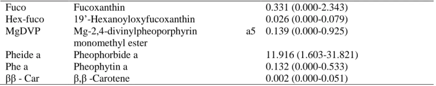
Table 2.3: Detected phytoplankton pigments concentrations throughout the experiment (mean and minimum-maximum values)

Abbreviation Pigment Average and range of concentrations

(mg m-3₎ Chl a Chlorophyll a 0.206 (0.000-1.889) TChl a Total Chlorophyll a 0.279 (0.000-2.549) Chlide a Chlorophyllide a 0.042 (0.000-0.589) Chl b Chlorophyll b 0.054 (0.000-0.136) Chl c2 Chlorophyll c2 1.247 (0.061-3.949) Chl c3 Chlorophyll c3 0.065 (0.000-0.205) Diadino Diadinoxanthin 0.010 (0.000-0.095)

11

The CHEMTAX chemical taxonomy software (version 1.95; Mackey et al., 1996; Wright et al., 1996) was used to estimate the relative contribution of phytoplankton groups to total chlorophyll a biomass, hence calculating their relative abundances. This software, given an initial pigment ratio matrix, uses factor analysis and a steepest descent algorithm to calculate the best fit to the data acquired through HPLC, as shown in Mackey et al. (1996).

Four phytoplankton classes were considered (Diatoms-1, Dinoflagellates-4, Chrysophyceae and Haptophyceae) based on identified pigments (HPLC) and main taxa from microscopy. The pigments chosen were chl c3, fucoxanthin, hex-fuco (19' – hexanoyloxyfucoxanthin), chl b and chl a and its initial pigment ratios to chlorophyll a were obtained from previous several CHEMTAX studies (diatoms-1 - Gibb et al., 2001; dinoflagellates-4 - Lampert et al., 2016; Chrysophyceae - Laza-Martinez et al., 2007; Haptophyceae - Seoane et al., 2009). The relatively low number of pigments loaded into the software is a result of the low pigment variability in the collected water sample (Table 2.). Diatoms-1 were included due to the detection of high abundances of Chaetoceros sp. Dinoflagellates-4 inclusion was prompted by the presence of Gymnodimnium sp. cells and the absence of peridinin, while Chrysophyceae were the most abundant flagellate group in microscopy samples. Pigment data was divided in two sub-matrices (N-limited and P-limited) according to which treatment the samples were subjected. These sub-matrices did not include any control samples as it would increase the error, thus affecting the CHEMTAX analysis. The initial and final ratios are shown in.

Table 2.4: Initial and final pigments-to-chl a ratio matrices in CHEMTAX analysis.

Taxa Chl c3 Fuco Hex-fuco Chl b Chl a

Initial ratios

Diatoms-1 0 0,818 0 0 1

Dinoflagellates-4 0 0 0 0,741 1

Chrysophyceae 0,250 0,970 0 0 1

Haptophyceae 0,229 0,316 0,534 0 1

Final ratios (N-limited)

Diatoms-1 0 0,727 0 0 1

Dinoflagellates-4 0 0 0 0,738 1

Chrysophyceae 0,522 0,271 0 0 1

Haptophyceae 0,128 0,208 0,424 0 1

Final ratios (P-limited)

Diatoms-1 0 0,637 0 0 1

Dinoflagellates-4 0 0 0 0,730 1

Chrysophyceae 0,498 0,285 0 0 1

Haptophyceae 0,127 0,215 0,428 0 1

In order to optimize the CHEMTAX analysis, 60 pigment ratios matrices were generated by multiplying each cell of the initial ratio matrix by a randomly determined factor (Wright et al., 2009). The final matrix consisted in the average of the six ratio output matrices with lowest residual or root

12

mean square errors (< 0.05), thereby obtaining the best results. All the analyses were done following the proceedings of Wright et al. (2009).

3. RESULTS

3.1. Pre-experiment environmental conditions

Sea surface temperature, as measured by the SNPP VIIRS mission, for the two weeks preceding the experiment near the water collection station was between 12º-14ºC (Figure 3.1), similar values to the 14ºC measured in the Day 0 sample. The low SST detected along the Chilean Western coast are typical of a coastal upwelling event, a pattern which is corroborated by high chlorophyll a values in the same time-period. Plus, Figure 3.2 displays upwelling-favourable winds recorded near the sampling station with speed ranging from 5-10 m/s.

Figure 3.1: SNPP VIIRS mean sea surface temperature (SST; ºC) and chlorophyll a concentration (CHL; mg m-3_{) in the}

Chilean coast on the weeks preceding the experiment (on the left: 9th_-16th_{, on the right: 16}th_-23th _{of October 2013). The red}

13

Figure 3.2: Mean WindSat wind vector direction and speed (ms-1_{) in the South-East Pacific on the weeks preceding the}

experiment (12th_-19th _{and 19}th_-26th _{of October 2013). The red triangle marks the location of the water collection station. Note}

that the three round black patches on the left side of the images correspond to the Desventuradas and Juan Fernández archipelagoes.

14

Thus, the environmental conditions gathered suggest upwelling occurrence, particularly in the week of 9th_-16th _{October (Figure 3.1). Nutrient-rich waters due to upwelling are generally limited in}

nitrogen (i.e. with low N/P ratios), a view which is supported by the measured N/P ratio in Day 0 (0.83).

3.2. Chlorophyll and nutrients dynamics

Figure 3.3: Mean chlorophyll a concentrations (mg.m-3_{) from Day 0 to Day 6 for both treatments and control. Error bars}

shown are standard errors (SE). Note that the dotted, dashed and solid lines respectively correspond to Control, N-limited and P-limited values.

Both treatments triggered an increase in chlorophyll a after the initial enrichment, reaching maximum chl a concentrations on Day 1 (Figure 3.3). Chl a values in the P-limited treatment (1.61 mg m-3_{) were more than twice as high as the measured in the N-limited (0.74 mg m}-3_{), also on Day 1.}

After Day 1, chlorophyll a decreased throughout the experiment. The only exception was after the second enrichment pulse (Day 3) in the N-limited treatment, where a small peak (0.13 mg m-3_{) was}

registered. In the P-limited treatment, no chl a increase occurred after the second enrichment event. Contrastingly, chlorophyll a values in control samples dropped on Day 1 and remained low. Despite showing a similar trend throughout the experiment, chlorophyll a concentrations were always higher in the P-limited treatment, particularly in the first days.

15

Figure 3.4: Dissolved inorganic nitrogen (NO2-+ NO3-) mean concentrations (µM) from Day 0 to Day 6 for both treatments

and control. Error bars shown are standard errors (SE). Note that the dotted, dashed and solid lines respectively correspond to Control, N-limited and P-limited values.

Figure 3.5: Phosphate (PO43−) mean concentrations (µM) from Day 0 to Day 6 for both treatments and control. Error bars

shown are standard errors (SE). Note that the dotted, dashed and solid lines respectively correspond to Control, N-limited and P-limited values.

DIN and phosphate concentrations, for both treatments, are shown in Figures 3.4 and 3.5. In the P-limited treatment, nitrate concentrations sharply decreased from the beginning of the experiment until it reached a minimum of 1.95 µM on Day 3. After the second enrichment stage, it increased to 22.9 µM on Day 4 and then started to drop again. Meanwhile, in the N-limited treatment, almost all nitrogen was consumed after Day 0. This condition remained constant until the end of the experiment, even though there was a minor peak (1.1 µM) on Day 4. Regarding phosphate, its concentration in the N-limited treatment slowly rose to 1.01 µM after a 44% decline on Day 1. However, its behaviour in the N-limited treatment was similar to the one shown by nitrate in the P-limited: a decrease on Day 1 followed by an increase after Day 3, when the enrichment pulse occurred. Yet, in this case, phosphate reached a maximum of 3.06 µM on Day 4.

16

Overall, DIN concentrations were considerably higher in the P-limited treatment than in the N-limited, where they were kept within low values due to higher nitrogen consumption than enrichment. Moreover, phosphate did not appear to have been consumed as much in the P-limited. Its concentration kept slowly rising after Day 1 in the P-limited treatment while nitrate was being consumed. DIN and phosphate concentrations in control samples remained low with a slight decrease and did not fluctuate. When comparing nutrient concentrations against chlorophyll a (Figure 3.3), it seems phytoplankton did not respond to the second enrichment pulse despite Figures 3.4 and 3.5 showing nitrate and phosphate consumption over that period.

3.3.

Nitrogen-to-phosphorus ratio

The N/P ratios measured in the experiment are shown in Figure 3.6. As N-limited treatment samples were mainly enriched in phosphate, nitrogen-to-phosphorus ratios registered in the N-limited treatment and in the control samples were, as expected, low, remaining below 0.4 after the experiment began (Day 1).

Figure 3.6: Mean nitrogen-to-phosphorus ratio (N:P) from Day 0 to Day 6 for both treatments and control. Error bars shown are standard errors (SE). Note that the dotted, dashed and solid lines respectively correspond to Control, N-limited and P-limited values.

In the P-limited treatment, despite the initial high N/P ratio (26.18), it rapidly fell to 2.91 on Day 3. After rising to 26.82 on Day 4 due to the second enrichment pulse, the N/P ratio started to decline again and reached 15.98 in the end of the experiment. Overall, N:P appeared to have a tendency for nitrogen limitation values (<16.0; Redfield, 1958), even when originally limited in phosphorus.

17

3.4.

Phytoplankton Community

Figure 3.7 shows phytoplankton cells abundance time series for all treatments. In both treatments, abundance peaked on Day 1 and declined after it. In the P-limited treatment, concentrations increased again on Day 3 and reached a maximum of 16.9 x 106 _{cells L}

-1 on Day 4.

From Day 4-6, abundance decreased to 10.9 x 106 _{cells L}

-1. In the N-limited treatment though, the

response to the second enrichment was clearer as cells abundance only increased on Day 4 (16.0 x 106

cells L-1). Higher abundances were always found in the P-limited treatment (predominantly N

enrichment). Cells abundances seem to confirm the initial increase in biomass already seen in chlorophyll a concentrations. However, cell abundance peaked in the second half of the experiment, showing an increase in biomass that is inconsistent with chl a data.

Figure 3.7: Mean total cell abundances (cells L-1_{) from Day 0 to Day 6 for both treatments and control. Error bars shown are}

standard errors (SE). Note that the dotted, dashed and solid lines respectively correspond to Control, N-limited and P-limited values.