Impacts of closure of a military base on a small island open economy

(1)

WORKING PAPER SERIES

CEEAplA WP No. 10/2006

Impacts of Closure of a Military Base on a Small

Island Open Economy

Mário Fortuna Ali Bayar Suat Sisik Cristina Mohora Sameer Rege July 2006

(2)

Impacts of Closure of a Military Base on a Small

Island Open Economy

Mário Fortuna

Universidade dos Açores (DEG)

e CEEAplA

Ali Bayar

Universite Libre de Bruxelles

Departement D’Economie Appliquee

EcoMod

Suat Sisik

Universite Libre de Bruxelles

Departement D’Economie Appliquee

EcoMod

Cristina Mohora

Universite Libre de Bruxelles

Departement D’Economie Appliquee

EcoMod

Sameer Rege

Universidade dos Açores (DEG)

e CEEAplA

Working Paper n.º 10/2006

Julho de 2006

(3)

CEEAplA Working Paper n.º 10/2006 Julho de 2006

RESUMO/ABSTRACT

Impacts of Closure of a Military Base on a Small Island Open Economy

Military bases are commonplace in many countries. Their economic impact on the neighbouring communities depends on their location and the level of integration of their activities on the local economies. Base closures or base activity reductions are also frequent as a consequence of military strategy alterations. The current paper seeks to analyse the economic impact of a US base located in the island of Terceira in the Azores. The base has been an important element of economic life in this island since the end of WWII. The changing geo-strategic map of the world has, along the second half of the twentieth century, led to changing roles of this base and consequent changes in the intensity of its activity. On the other hand discussions over the importance of the base for the local economy are recurrent in an attempt, on the part of the participants, to set forth arguments in favour or against the presence of military forces in the location. The current paper tries to contribute with a quantification of the economic impact of the base using a dynamic CGE model of the Azorean economy. A closure scenario is created and the impacts traced through various economic indicators including some sector detail. Estimates are made for the overall impact and for the impact on the island that houses the base.

Mário Fortuna

Departamento de Economia e Gestão Universidade dos Açores

Rua da Mãe de Deus, 58 9501-801 Ponta Delgada Ali Bayar

Universite Libre de Bruxelles

Departement D’Economie Appliquee Avenue Paul Heger 2

B-1000 Bruxelles Suat Sisik

(4)

Cristina Mohora

B-1000 Bruxelles Sameer Rege

Departamento de Economia e Gestão Universidade dos Açores

Rua da Mãe de Deus, 58 9501-801 Ponta Delgada

(5)

IMPACTS OF CLOSURE OF A MILITARY BASE ON A SMALL ISLAND OPEN ECONOMY Mário Fortuna* Ali Bayar** Suat Sisik** Cristina Mohora** Sameer Rege* Abstract

Military bases are commonplace in many countries. Their economic impact on the neighbouring communities depends on their location and the level of integration of their activities on the local economies. Base closures or base activity reductions are also frequent as a consequence of military strategy alterations. The current paper seeks to analyse the economic impact of a US base located in the island of Terceira in the Azores. The base has been an important element of economic life in this island since the end of WWII. The changing geo-strategic map of the world has, along the second half of the twentieth century, led to changing roles of this base and consequent changes in the intensity of its activity. On the other hand discussions over the importance of the base for the local economy are recurrent in an attempt, on the part of the participants, to set forth arguments in favour or against the presence of military forces in the location. The current paper tries to contribute with a quantification of the economic impact of the base using a dynamic CGE model of the Azorean economy. A closure scenario is created and the impacts traced through various economic indicators including some sector detail. Estimates are made for the overall impact and for the impact on the island that houses the base.

* CEEAplA, University of the Azores ** ECOMOD, ULB

(6)

1. Introduction

Military bases are commonplace in many countries. Their location has important economic impacts on the neighbouring communities and depends on the level of integration of their activities with the local economies. Base closures or base activity reductions are also frequent as a consequence of military strategy alterations. The current paper seeks to analyse the economic impact of a US base located in the island of Terceira in the Azores. The base has been an important element of economic life on this island since the end of WWII. The activity of the base reflects the changing geo-political situation in the second half of the twentieth century.

The improvements in defence technology coupled with a new equilibrium in global power politics have impacted the American strategy and perhaps their perception of the Lajes air base. This is reflected in the strength of the military personnel on the base and their approach to integration in the local community. Housing problems in the past were solved via rentals of the local housing but in the recent times there has been a shift to housing in the air base, this reducing the dependence on the local economy.

During the 1980’s, in addition to the direct impact of the base’s activity, its presence justified aid given to the regional government and other given directly to the national authorities. The monetary compensation for the use of the base is immediately quantified. Not so obvious are the impacts on local economic activity that results from the presence of the base.

Discussions over the importance and the impact of the base for the local economy are recurrent in an attempt, on the part of the participants, to advance arguments in favour or against its presence. The current paper tries to contribute with a quantification of the economic impact of the base using a dynamic CGE model of the Azorean economy. A closure scenario is created and the impacts traced through various economic indicators including some sector detail. Estimates are made for the overall impact and for the impact on the island that houses the base.

In what follows section 2 reviews the body of the literature on base closures using CGE models. Section 3 presents the main variables that characterize the impact of the base on the local economy. Section 4 reviews the main characteristics of a CGE model of the Azores. Section 5 reviews the results of calibration of the model and the results of the closure scenario developed. Section 6 presents some of the main conclusions that can be drawn from application of the model.

2. Analysing Base Closures with CGE Models

Sandra Hoffmann, Sherman Robinson, & Shankar Subramanian (1996) analyze the impact of defense cuts on the economy in California using a computable general equilibrium (CGE) model. Their focus is on the migration of factors from California to other states and the impact of this migration on the economy. CGE models are better suited to analyze the economy wide impact of these defense cuts and their study shows that the impacts are highly sensitive to the assumption of inter-state mobility.

(7)

Other studies have taken a less elaborate approach looking mostly at lost direct expenditures and jobs on an accounting approach and looking other social and environmental impacts.

The current research paper can be classified as a cut in defence expenditure and is more focussed on base closure on an island economy where the economic conditions are not very conducive to factor mobility, especially labour migration.

3. The Military Base in Terceira/Azores

The base in Terceira/Azores houses both US and Portuguese military activities. It comprises an airport adequate for landing any known type of aircraft, fuel storage tanks and port facilities. This base has been extensively used in various international conflicts, namely those that have occurred in the last half century and in the Middle East during recent times.

The impact of the American component of the base can be simulated by the model using data on the main variables. In the simulation undertaken here the relevant data collected characterizes expenditures on construction works and repair, employment and private consumption by the US military, servicemen and civilians.

Access of locals to purchases in the base’s stores can also be taken into consideration. It is common for some locals to make their purchases in the base stores at prices that are lower than those practiced in the local stores, for a wider variety of products. There are no good estimates for the total value of the purchases made in these stores, which is equivalent to purchasing the goods abroad. Given that there are no good estimates of the values involved, two scenarios will be created to test the impact of these “imports”: one where the import effect is zero, the reference scenario and one in which 50% of the income is spent on these “foreign” stores.

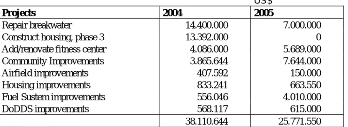
The main elements of the date on the activity of the US military are summarized in tables 1 and 2. Table 1 provides an estimate of the value (in US Dollars) of the construction works and repair commissioned by the Lajes Field Base for 2004 and for 2005.

Table 1 Construction works and repair commissioned by the Lajes Field base

US$

Projects 2004 2005

Repair breakwater 14.400.000 7.000.000

Construct housing, phase 3 13.392.000 0

Add/renovate fitness center 4.086.000 5.689.000

Community Improvements 3.865.644 7.644.000

Airfield improvements 407.592 150.000

Housing improvements 833.241 663.550

Fuel Sustem improvements 556.046 4.010.000

DoDDS improvements 568.117 615.000

38.110.644 25.771.550

Source: U.S. Air force

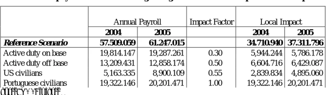
An evaluation of the local consumption expenditure by the US base staff in Azores is given in Table 2.

(8)

To estimate the local impact of the Lajes Field Base two scenarios are created. On the first scenario it is assumed that 30 per cent of the payroll of active duty personnel living on base is spent outside the base. For the active duty personnel living off base this figure is estimated at 50 per cent, and for US civilians living it is assumed at 55%. For the Portuguese civilians working on base, two scenarios are considered: one in which they spend 100 per cent of their income off base and one in which they spend only 50 per cent off base. This second scenario tries to take into account the mentioned fact that many civilians purchase goods in the base stores supplied by the US military.

Table 2 Annual payroll and estimates regarding the loss in terms of private consumption

Annual Payroll Impact Factor Local Impact

2004 2005 2004 2005

Reference Scenario 57.509.059 61.247.015 34.710.940 37.311.796

Active duty on base 19,814.147 19,287.261 0.30 5,944.244 5,786.178

Active duty off base 13,209.431 12,858.174 0.50 6,604.716 6,429.087

US civilians 5,163.335 8,900.109 0.55 2,839.834 4,895.060

Portuguese civilians 19,322.146 20,201.471 1.00 19,322.146 20,201.471

The closure of the US component of the Lajes Field base would have direct and indirect impacts on the economy of the Azores through the following four channels:

The reduction in the demand for construction works and repair;

The employment loss of the Portuguese civilians working on the base, which leads to a loss in the labour income and consumption demand both domestic and foreign, namely the demand of goods from the base’s stores;

The loss in the consumption demand from the US active duty personnel living on base and off base;

The loss of the rents of local lodging contracted quarters.

The difference of financial impact between the two scenarios is about US$10million, a variation of about 28%.

4. A CGE Model of a Small Island Economy

4.1 Model Description

The model is a static multi-sector computable general equilibrium model (CGE), which incorporates the economic behaviour of four economic agents: firms, households, government and the rest of the world. All economic agents are assumed to adopt an optimizing behaviour under relevant budget constraints and all markets operate under the perfect competition assumption. The goods-producing sectors, consisting of both public and private enterprises, are disaggregated into 16 sectors1. The model distinguishes 16 types of commodities, such that each sector produces one homogenous commodity. With regard to the rest of the world the economy is treated as a small open economy with no influence on (given) world market prices.

The model is calibrated on the regional Social Accounting Matrix for 1998. The model has been solved by using the general algebraic modelling system GAMS (Brooke et al., 1998).

1

(9)

The following conventions are adopted for the presentation of the model. Variable names are given in capital letters; small letters denote parameters calibrated from the database (SAM) and elasticity parameters. Subscript sec stands for an identifier of one of the 16 production activities and one of the 16 commodities. Subscript ct stands for an identifier of the wholesale and retail trade services. Subscript nct stands for an identifier of one of the 15 commodities (except wholesale and retail trade services).

4.2 Firms

The CGE model does not take into account the behaviour of individual firms, but of groups of similar ones aggregated into sectors. The model distinguishes 16 perfectly competitive production sectors (summarized in section 4.11).

The usual assumption for such a model is that producers operate on perfectly competitive markets and maximize profits (or minimize costs) to determine optimal levels of inputs and output. For example, for the firms operating internationally, the world market dictates the output price to a large extent, so, for an optimal outcome they have to produce as efficiently as possible. Some other firms are constrained in the costs level by domestic competitors. Thus, the optimizing producers minimize their production costs at every output level, given their production technology. Furthermore, production prices equal average and marginal costs, a condition that implies profit maximization for a constant returns to scale technology.

Gross output for each sector is determined from a nested production structure. At the outer nest producers are assumed to choose intermediate inputs and a capital-labour (KL) bundle, according to a Leontief production function, which assume an optimal allocation of inputs. At the second nest, producers choose the optimal level of labour and capital, according to a constant elasticity of substitution (CES) function which assumes substitution possibilities between labour and capital. Rigidities in the labour market are further introduced by the inter-sectoral wage differentials. The inter-sectoral wage differentials are derived as the ratio between the sectoral wage rate and the average wage rate at the national level (Dervis, De Melo and Robinson, 1982).

The demand equations for intermediate inputs, labour and capital and the corresponding zero profit conditions for these sectors are provided in section 4.12, equations (4.12.5-4.12.9). The nested structure and the functional forms used by these sectors are further given in figure 1. Gross output KL bundle Le ontie f C ES Labour C apital

Inte rme diate inputs

(10)

Figure 1: The nested Leontief and CES production technology

Treated at an aggregate level, firms receive income from sales of goods; they purchase intermediate inputs, make wage payments and save (see equation (4.12.10), section 4.12).

4.3 Households

The households receive income from labour and a fixed share of the capital income and transfers from the government as unemployment benefits (see equation (4.12.2), section 4.12) and pay taxes on income to government and save a fixed fraction of net (money) income (see equation (4.12.3), section 4.12). Further, households’ budget devoted to consumption of commodities is given by the total income minus the taxes and savings (see equation (4.12.4), section 4.12). A schematic representation of households’ decisions is given in figure 2.

The optimal allocation between the consumption commodities ( C_sec) is given by maximizing a Stone-Geary utility function:

Hsec U( C_sec) ( C_sec H_sec)

sec

α µ

= ∏ − (1)

subject to the budget constraint:

CBUD=(1-tsc_sec) (1+tc⋅ _sec)⋅P_sec⋅C_sec (2) where: _sec

sec H 1

α =

∑ .

sec

C represents the consumption of commodity sec by the households, P_sec is the consumer price net of taxes for the commodity sec, µ_sec is the minimum (subsistence) level of consumption of commodity sec by the households, and αH_sec is the income elasticity of the demand for commodity sec.

Sixteenth categories of consumer goods are distinguished. As already explained, each production sector is assumed to produce one homogenous commodity. Thus, the classification of the commodities follows the classification of the production sectors.

(11)

C api tal su ppl y Labor su ppl y In com e from capi tal Labor de m an d Un e m pl oym e n t In com e from l abor Un e m pl oym e n t be n e fi ts In com e Taxe s on i n com e Hou se h ol d savi n gs C om m odi ti e s (16 type s) C on su m pti on bu dge t

Figure 2: Decision structure of the households

Consumption is valued at consumer prices (1-tsc_sec) (1+tc⋅ _sec)⋅P_sec, which incorporate taxes on consumption (tc_sec) and subsidies on consumption ( tsc_sec).

After some rearrangements, the optimization process generates the demand equations for consumption commodities (see equations (4.2.12), section 4.12)2.

To evaluate the overall change in consumer welfare we use the equivalent variation in income( EV ), which is based on the concept of a money metric indirect utility function (Varian, 1992):

sec

H sec sec sec

sec sec PZ ( 1 tc0 ) ( 1 tsc0 ) EV = (V-VZ) H α α ⎡ ⋅ + ⋅ − ⎤ ⋅ ∏ ⎢ ⎥ ⎣ ⎦ (3)

The indirect utility function of the LES function in the counter-factual (policy scenario) equilibrium (V ) is defined as:

[

]

sec

sec sec sec sec sec

H sec sec sec sec sec V = CBUD- P ( 1 tc ) ( 1 tsc ) H H /(P ( 1 tc ) ( 1 tsc ))α µ α ⎡ ⎤ ⋅ + ⋅ − ⋅ ⋅ ∑ ⎢ ⎥ ⎣ ⎦ ⋅ + ⋅ − ∏ (4)

and the indirect utility function of the LES function in the benchmark equilibrium (VZ )

is given by:

2

The Linear Expenditure System (LES) was developed by Stone (1954) and represents a set of consumer demand equations linear in total expenditure.

(12)

[

]

sec

H sec sec sec sec sec VZ = CBUDZ- PZ ( 1 tc0 ) ( 1 tsc0 ) H H /(PZ ( 1 tc0 ) ( 1 tsc0 )) α µ α ⎡ ⎤ ⋅ + ⋅ − ⋅ ⋅ ∑ ⎢ ⎥ ⎣ ⎦ ⋅ + ⋅ − ∏ (5)

whereCBUDZ reflects the household’s budget available for consumption in the benchmark equilibrium,PZ_sec is the price of commodity sec in the benchmark and

sec

tc0 and tsc0_sec are the consumption tax rate and the subsidy rate in the benchmark equilibrium, respectively.

Equivalent variation measures the income needed to make the household as well off as she is in the new counter-factual equilibrium (policy scenario) evaluated at benchmark prices. Thus, the equivalent variation is positive for welfare gains from the policy scenario and negative for losses (Harrison and Kriström, 1997).

4.4 Government

Government revenues (TAXR) consist of taxes on households’ income, consumption taxes, taxes on investment goods and taxes on production plus transfers received by the government from the rest of the world:

sec sec sec sec sec sec sec sec

sec sec sec sec TAXR = ty YH + (P C (1-tsc ) tc +XD PD tp )+ P I tcinv +ER TRGW ⋅ ⋅ ⋅ ⋅ ⋅ ⋅ ⋅ ⋅ ⋅

∑

(6)

where ty is the tax rate on households income (YH ), tp_sec is the tax on production of sector sec and tcinv_sec is the tax rate on investment good sec. XD_sec represents the gross output of sector sec, where its price is given by PD_sec, and I_sec reflects the demand for the investment commodity sec. The transfers received by the government from the rest of the world (TRGW) are transformed in domestic currency by multiplying them with the exchange rate (ER).

Government expenditures (GEXP) consists of disposable budget for current consumption

(CGBUD), unemployment benefits to the households’ and subsidies on consumption and

production:

sec sec sec sec sec sec sec

GEXP = CGBUD+trep PL UNEMP+⋅ ⋅

∑

(P ⋅C ⋅tsc +XD ⋅PD ⋅tsp ) (7)

where UNEMP represents the number of unemployed, PL is the average wage rate, trep

is the replacement rate out of the average wage rate, tsc_sec is the subsidy rate on consumption of commodity sec and tsp_sec is the subsidy rate on production of sector sec.

Thus, government savings are given by the difference between government revenues and government expenditures:

SG = TAXR-GEXP (8)

The optimal consumption of commodities by the government is given by the maximization of a Cobb-Douglas utility function:

sec sec CG U( CG ) _CGsec sec α = ∏ (9)

(13)

subject to the budget constraint: sec sec sec CGBUD =

∑

CG ⋅P (10) With: _sec sec CG 1 α =

∑ . The optimization process yields the demand equations for each type of commodity (see equation (4.12.13), section 4.12).

4.5 Foreign trade

The specification of foreign trade is based on the small-country assumption, which means that the country is a price taker in both its imports and exports markets. As a result, both world import prices and world export prices are exogenously fixed. Two main groups of trading partners are distinguished in the model: the Mainland and the rest of the world.

The assumption of limited substitution possibilities between domestically produced and imported goods, which goes back to Armington (1969), is now a standard feature of applied models and will also be adopted here. It indicates that domestic consumers use composite goods ( X_sec) of imported and domestically produced goods, according to a CES function:

sec sec

A A

sec sec sec sec sec sec A 1 A sec sec X aA ( A1 MML A2 MROW A3 XDD ) ρ ρ ρ ρ γ γ γ − − − − = ⋅ ⋅ + ⋅ + ⋅ (11)

Minimizing the cost function:

sec sec sec sec sec sec sec sec sec sec

Cost ( MML ,MROW , XDD ) PMML MML PMROW MROW PDD XDD

= ⋅ +

⋅ + ⋅ (12)

subject to (11), yields the demand equations for imports from Mainland ( MML_sec), for imports from the rest of the world ( MROW_sec) and domestically produced goods

sec

( XDD ) (see equations (4.12.16-4.12.18), section 4.12); where aA_sec is the efficiency

parameter, γA1_sec, γA2_sec, γA3_sec are the distribution parameters and the elasticity of substitution between imports from different regions and domestically produced goods

sec

( Aσ ) is given by 1 ( 1+ρA_sec). PMML_secis the domestic price of imports of commodity sec from Mainland including trade margins, PMROW_sec is the domestic price of imports of commodity sec from the rest of the world including trade margins, and PDD_sec is the price of domestically produced commodity sec delivered to the domestic market also including trade margins.

The corresponding zero profit condition for the CES function is given by:

P ⋅X = PMML ⋅MML + PMROW ⋅MROW +PDD ⋅XDD (13)

where P_sec is the composite price of commodity sec net of taxes.

A limited substitution is also assumed to exist between goods produced for the domestic market ( XDD_sec), exports to Mainland ( EML_sec) and exports to the rest of the world

sec

(14)

sec sec sec sec

T T

sec sec sec sec sec sec T 1 T sec sec XD aT ( T1 EML T 2 EROW T 3 XDD ) ρ ρ ρ ρ γ γ γ − − − − = ⋅ ⋅ + ⋅ + ⋅ (14)

where aT_sec is the efficiency parameter, γT1_sec, γT 2_sec, γT 3_sec are the distribution parameters, and the elasticity of substitution ( Tσ _sec) between exports to different regions and domestically produced goods delivered to domestic market is given by

sec

1 ( 1+ρT ).

By maximizing the revenue function of the producer:

Re venue ( EML ,EROW , XDD ) PEML EML PEROW EROW PDS XDD

= ⋅ +

⋅ + ⋅ (15)

subject to (14) we derive the demand equations for exports and domestically produced goods (see equations (4.12.20-4.12.22), section 4.12), where PEML_sec is the domestic price of exports of sector sec to the Mainland, PEROW_sec is the domestic price of exports of sector sec to the rest of the world, and PDS_sec is the price of domestic output of sector sec delivered to domestic market excluding trade margins.

The zero profit condition for the CET function is further given by:

PD ⋅XD = PEML ⋅EML +PEROW ⋅EROW + PDS ⋅XDD (16) where PD_sec is the price of output produced by sector sec. Both exports and domestic output delivered to the domestic market are valued at basic prices, PEML_sec, PEROW_sec

and PDS_sec.

The balance of payments is now determined as all international incoming and outgoing payments have been taken into account:

sec

(MML PWMMLZ +MROW PWMROWZ ) =

( EML PWEMLZ +EROW PWEROWZ ) TRGW+SW+LW PLWZ

⋅ ⋅

∑

⋅ ⋅ + ⋅

∑

(17)

The surplus/deficit of the balance of payments ( SW ), expressed in foreign currency, is determined by the difference between imports and exports, valued at world prices, the transfers received by the government from the rest of the world (TRGW) and the labor income from non-residential firms (LW PLWZ)⋅ , where PWMMLZ_secis the foreign price of imports of commodity sec from the Mainland, PWMROWZ_sec is the foreign price of imports of commodity sec from the rest of the world, and PWEMLZ_sec, PWEROWZ_secare the foreign prices of exports of sector sec to the Mainland and to the rest of the world, respectively.

4.6 Investment demand

Total national savings are given by:

sec sec

(15)

where SH are the households’ savings, SF firms savings, SG government savings and

sec

DEP is the depreciation of the capital stock. Depreciation is modelled as a fixed share of capital stock (see equation 4.12.26, section 4.12).

The demand for investment commodities by type of commodity ( I_sec) is modelled in a simple way, by maximizing a Cobb-Douglas utility function:

sec

I sec sec

sec

U( I )= ∏Iα (19)

subject to the budget constraint:

S−

∑

SV ⋅P =

∑

I ⋅P ⋅ +( 1 tcinv ) (20)

with _sec

sec I 1

α =

∑ , where SV_{s ec} are the changes in stocks of commodity sec and tcinv_sec

is the tax rate on investment commodity sec. Changes in stocks are modelled in this case as a fixed share out of supply of commodities (see equation (4.12.27), section 4.12). Further, the maximization process yields the demand equations for investment commodities by type of commodity (see equation (4.12.28), section 4.12). The price of the composite investment commodity is further given by:

sec

I sec sec sec sec

PI = ∏[(P ⋅(1+tcinv ) ) / Iα ]α (21)

4.7 Price equations

A common assumption for CGE models, which has also been adopted here, is that the economy is initially in equilibrium with the quantities normalized in such a way that prices of commodities equal unity. Due to the homogeneity of degree zero in prices, the model only determines relative prices. Therefore, a particular price is selected to provide the numeraire price level against which all relative prices in the model will be measured. In this case, the GDP deflator (GDPDEF) is chosen as the numeraire.

Different prices are distinguished for all producing sectors, exports and imports. The domestic price of exports to Mainland ( PEML_sec) reflects the price received by the domestic producers for selling their output to the Mainland, where PWEMLZ_sec is the foreign price of exports to Mainland and ER is the exchange rate. The cost of trade inputs further reduces the domestic price received by the producers:

sec sec ct,sec ct ct

PEML =PWEMLZ ⋅ER−

∑

tcoeml ⋅P (22)

where tcoeml_{ct ,sec} is the quantity of commodity ct as trade input per unit of commodity sec exported and Pctrepresents the price of commodity ct. Commodity ct is in fact the

wholesale and retail sale commodity. In a similar way is defined the domestic price of exports to the rest of the world (see equation (4.12.38), section 4.12).

The domestic price of imports from Mainland ( PMML_sec) is determined by the foreign price of imports from Mainland ( PWMMLZ_sec), the exchange rate, and the cost of trade inputs for imports:

(16)

where tcomml_ct,sec is the quantity of commodity ct as trade input per imported unit of commodity sec.

The model distinguishes the price of domestic output supplied to domestic market paid by the consumers (PDD_i) and the price received by the producers (PDS_i). The difference between the two prices is represented by the cost of trade inputs for domestic output delivered to domestic market:

PDD =PDS +

∑

tcod ⋅P (24)

where tcod_ct,sec is the quantity of commodity ct as trade input per unit of commodity sec delivered to the domestic market.

The consumer price index (INDEX) used in the model is of the Laspeyres type and is defined as:

sec sec sec sec sec INDEX = P CZ (1+tc ) (1-tsc ) / PZ CZ (1+tc0 ) (1-tsc0 ) ⋅ ⋅ ⋅ ⎡ ⎤ ⎣ ⎦ ⋅ ⋅ ⋅ ⎡ ⎤ ⎣ ⎦

∑

(25)

Furthermore, GDP deflator is defined as the ratio of GDP at current market prices to GDP at constant prices (see equation (4.12.42), section 4.12).

4.8 Labour market

Labour services are used by firms in the production process (see equation (4.12.7), section 4.12). The model also allows for endogenous unemployment. Thus, the average wage rate paid by the firms is a function of consumer prices and the unemployment rate, as follows:

(

)

( ) /( ) 1

PL INDEX PLZ INDEXZ

beta UNEMP LSR UNEMPZ LSRZ

− =

⋅ − (26)

where LSR is the domestic labour supply, PL is the average wage rate in the current year and beta is a parameter. PLZ, INDEXZ, UNEMPZ and LSRZ represent the average wage rate, the consumer price index, the unemployment level and the domestic labour supply in the base year, respectively.

A labour supply curve, which assumes a positive correlation between the domestic labour supply and the real average wage rate:

elasLS

LSR = LSRZ ((PL INDEXZ)/(PLZ INDEX))⋅ ⋅ ⋅ (27)

is used to endogenize labour supply in the model, where elasLS is the real wage elasticity of labour supply.

Labour market is closed by changes in unemployment:

sec sec

LSK = LSR - UNEMP

∑

(28)

where LSK_sec is the labour demand by sector sec. Further, total labour supply (LS) is given by:

LS=LSR LW+ (29)

(17)

4.9 Market clearing equations

Equilibrium in the product, capital and labour markets requires that demand equals supply at the prevailing prices (taking into account unemployment for the labour market). The clearing equation for the labour market has already been presented above (see equation (28)).

Similarly, the sum of demand for intermediate inputs nct (excluding the wholesale and retail trade commodity) of sector sec ( io_nct,sec⋅XD_sec), of demand for government and households consumption, of demand for investment goods and inventories must equal the supply of the composite good nct from domestic deliveries and imports (X_nct):

nct,sec sec nct nct nct nct nct sec

io ⋅XD +C +I +SV +CG = X

∑ (30)

For the wholesale and retail trade commodity the market clearing equation is given by:

ct,sec sec ct ct ct ct ct ct sec

io ⋅XD +C +I +SV +CG +MARG = X

∑

(31)

where MARG_ct is the demand for trade services (Löfgren, Harris and Robinson, 2002). Total demand for trade services is further given by the sum of demand for trade services generated by the domestic output delivered to the domestic market, of the demand for trade services generated by the imports, and of the demand for trade services generated by the exports:

ct ct,sec sec ct,sec sec sec

ct,sec sec ct,sec sec ct,sec sec

MARG = (tcod XDD +tcomml MML +

tcomrow MROW +tcoeml EML +tcoerow EROW )

⋅ ⋅

⋅ ⋅ ⋅

∑

(32) Further, capital stock is fixed by sector; therefore the equation for the clearing of the capital market has been dropped.

4.10 Closure rules

The closure rule refers to the manner in which demand and supply of commodities, the macroeconomic identities and the factor markets are equilibrated ex-post. Due to the complexity of the model, a combination of closure rules is needed. The particular set of closure rules should also be consistent, to the largest extent possible, with the institutional structure of the economy and with the purpose of the model.

To balance the number of endogenous variables and the number of independent equations in the model, additional assumptions are needed. Therefore, the transfers received by the government form the rest of the world and the labour income from non-residential firms is exogenously fixed in real terms. Further, in order to achieve the clearing of the labour market, inter-sectoral mobility of labour is assumed. However, the presence of unemployment introduces rigidities in the labour market. The unemployment is endogenously determined through a wage curve. Labour supply is endogenously determined through a labour supply curve. On the capital market the sectoral capital stock is exogenously fixed, introducing rigidities.

The most widely accepted macro closure rule for CGE models implies the assumption that investment and savings balance. In the model, the investment is assumed to adjust to the available domestic and foreign savings. This reflects an economy in which savings form a binding constraint. The interest rate is assumed to effectively balance the supply and demand for investments, even if the specific mechanism is not incorporated

(18)

in the model. This macro closure rule is neoclassical in spirit. However, the fact that the model allows for unemployment introduces a Keynesian element. As already mentioned, in models of this size it is not uncommon that a few closure rules are combined to get as close as possible to a realistic representation of the economy.

The government behaviour is modelled through an optimization process, which yields the optimal allocation of governments’ consumption by type of commodity. The budget deficits/surpluses of the government are fixed as a share of GDP. For the external sector, the surplus/deficit of the balance of payments is fixed and the endogenous exchange rate brings the balance of payments into equilibrium.

Gross domestic product is obtained at both constant prices and current market prices (see equations 4.12.43-4.12.44, section 4.12). According to Walras’ law if (n-1) markets are cleared the nth one is cleared as well. Therefore, in order to avoid over-determination of the model, balance of payments equation (equation 17) has been dropped. However, the system of equations guarantees, through Walras’ law, that its balance is equal to the difference between the exports and imports and the transfers from the rest of the world.

4.11 Classification of the production sectors in the SAM Table 3: Classification of the production sectors in the SAM

Code Azores core model

Classification of the production sectors in the SAM and in AzoresMod NACE Division

sec1 Products of agriculture, hunting and forestry A

sec2 Fish B

sec3 Products from mining and quarrying C

sec4 Manufactured products D

sec5 Electrical energy, gas, steam and hot water E

sec6 Contruction work F

sec7

Wholesale and retail trade services; repair services of motor vehicles,

motorcycles and personal and household goods G

sec8 Hotel and restaurant services H

sec9 Transport, storage and communication services I

sec10 Financial intermediation services J

sec11 Real estate, renting and business services K

sec12

Public administration and defence services, compulsory social security

services L

sec13 Education services M

sec14 Health and social services N

sec15 Other community, social and personal services O

sec16 Private household with employed persons P

4.12 Model equations 4.12.1 Households

sec sec sec sec sec sec sec sec sec sec c sec c sec c sec c

sec c P C ( 1 tc ) ( 1 tsc ) P H ( 1 tc ) ( 1 tc ) H ( CBUD H P ( 1 tc ) ( 1 tsc ) ) µ α µ ⋅ ⋅ + ⋅ − = ⋅ ⋅ + ⋅ − + ⋅ −

∑

⋅ ⋅ + ⋅ − (4.12.1)

sec sec YH = aich KSK RK LSK wdif PL trep PL UNEMP+PLWZ ER LW ⋅ ⋅ + ⋅ ⋅ + ⋅ ⋅ ⋅ ⋅

∑

(4.12.2) ( ) SH =mps YH ty YH⋅ − ⋅ (4.12.3)

(19)

CBUD = YH-ty YH-SH ⋅ (4.12.4)

4.12.2 Firms sec sec sec

aKL ⋅XD = KL (4.12.5)

sec sec sec sec sec sec secc,sec sec secc secc

(1-tp +tsp ) PD⋅ ⋅XD = KL ⋅PKL +

∑

io ⋅XD ⋅P (4.12.6)

sec sec sec P ( P -1)

P

sec sec sec sec sec sec

LSK = KL ⋅[ PKL /(PL wdif⋅ )]σ ⋅γP2σ ⋅aPσ (4.12.7)

sec sec sec P ( P -1)

P

KSK = KL ⋅(PKL /(RK +d ⋅PI))σ ⋅γP1σ ⋅aPσ (4.12.8)

PKL ⋅KL = RK ⋅KSK +DEP ⋅PI+PL LSK⋅ ⋅wdif (4.12.9)

sec sec sec

SF = aicf⋅

∑

KSK ⋅RK (4.12.10)

4.12.3 Government

sec sec sec

TAXR = ty YH + [P C (1-tsc ) tc +XD PD tp + P I tcinv ]+ER TRGW ⋅ ⋅ ⋅ ⋅ ⋅ ⋅ ⋅ ⋅ ⋅

∑

(4.12.11)

GEXP = CGBUD+trep PL UNEMP+⋅ ⋅

∑

[P ⋅C ⋅tsc +XD ⋅PD ⋅tsp ] (4.12.12)

sec sec sec

P ⋅CG = Gα ⋅CGBUD (4.12.13) SG = TAXR-GEXP (4.12.14) RATIO = SG/GDPC (4.12.15) 4.12.4 Foreign trade sec sec sec

sec sec sec sec sec sec

A (1 - A ) A

sec sec sec sec sec sec sec A (1 - A ) A (1 - A ) A /(1 - A )

MML = (X /aA ) ( A1 /PMML ) [ A1 PMML + A2 PMROW + A3 PDD ] σ σ σ σ σ σ σ σ σ γ γ γ γ ⋅ ⋅ ⋅ ⋅ ⋅ (4.12.16) sec sec sec

A (1 - A ) A

sec sec sec sec sec sec sec A (1 - A ) A (1 - A ) A /(1 - A )

MROW = (X /aA ) ( A2 /PMROW ) [ A1 PMML +

A2 PMROW + A3 PDD ] σ σ σ σ σ σ σ σ σ γ γ γ γ ⋅ ⋅ ⋅ ⋅ ⋅ (4.12.17) sec sec sec

A (1 - A ) A

sec sec sec sec sec sec sec A (1 - A ) A (1 - A ) A /(1 - A )

XDD = (X /aA ) ( A3 /PDD ) [ A1 PMML + A2 PMROW + A3 PDD ] σ σ σ σ σ σ σ σ σ γ γ γ γ ⋅ ⋅ ⋅ ⋅ ⋅ (4.12.18)

P ⋅X = PMML ⋅MML +PMROW ⋅MROW +PDD ⋅XDD (4.12.19)

sec sec

sec

T (1 - T ) T

sec sec sec sec sec sec sec T (1 - T ) T (1 - T ) T /(1 - T ) sec sec sec sec

EML = (XD /aT ) ( T1 /PEML ) [ T1 PEML +

T2 PEROW + T3 PDS ] σ σ σ σ σ σ σ σ σ γ γ γ γ ⋅ ⋅ ⋅ ⋅ ⋅ (4.12.20) sec sec sec

T (1 - T ) T

sec sec sec sec sec sec sec T (1 - T ) T (1 - T ) T /(1 - T )

EROW = (XD /aT ) ( T2 /PEROW ) [ T1 PEML +

T2 PEROW + T3 PDS ] σ σ σ σ σ σ σ σ σ γ γ γ γ ⋅ ⋅ ⋅ ⋅ ⋅ (4.12.21) sec sec sec

T (1 - T ) T

sec sec sec sec sec sec sec T (1 - T ) T (1 - T ) T /(1 - T ) sec sec sec sec

XDD = (XD /aT ) ( T3 /PDS ) [ T1 PEML + T2 PEROW + T3 PDS ] σ σ σ σ σ σ σ σ σ γ γ γ γ ⋅ ⋅ ⋅ ⋅ ⋅ (4.12.22)

(20)

PD ⋅XD = PEML ⋅EML + PEROW ⋅EROW +PDS ⋅XDD (4.12.23)

4.12.5 Investments

sec

I sec sec sec sec

PI =

∏

[(P ⋅(1+tcinv ))/ Iα ]α (4.12.24)

sec sec

S = SH + SF + SG - SW ER + ⋅

∑

DEP ⋅PI (4.12.25)

sec sec sec

DEP = d ⋅KSK (4.12.26)

sec sec sec

SV = svr ⋅X (4.12.27)

sec sec sec sec secc secc secc (1+tcinv ) P⋅ ⋅I = Iα ⋅(S-

∑

SV ⋅P ) (4.12.28) 4.12.6 Labor market sec sec LSK = LSR - UNEMP

∑

(4.12.29) LS=LSR LW+ (4.12.30) ( ) ( )

(

/

)

elasLS LSR LSRZ= ⋅ PL INDEXZ⋅ PLZ INDEX⋅ (4.12.31) (PL / INDEX / PLZ / INDEXZ) ( )− =1 beta⋅

(

(UNEMP / LSR / UNEMPZ / LSRZ) ( )−1

)

(4.12.32)

4.12.7 Market clearing

ct ct,sec sec ct,sec sec sec

ct,sec sec ct,sec sec ct,sec sec

MARG = (tcod XDD +tcomml MML +

tcomrow MROW +tcoeml EML +tcoerow EROW )

⋅ ⋅ ⋅ ⋅ ⋅ ∑ (4.12.33) nct,sec sec nct nct nct nct nct sec io ⋅XD +C +I +SV +CG = X ∑ (4.12.34) ct,sec sec ct ct ct ct ct ct sec io ⋅XD +C +I +SV +CG +MARG = X

∑

(4.12.35) 4.12.8 Price equations

sec sec sec sec sec INDEX [ P CZ ( 1 tc ) ( 1 tsc )] / [ PZ CZ ( 1 tc0 ) ( 1 tsc0 )] = ⋅ ⋅ + ⋅ − ⋅ ⋅ + ⋅ −

∑

(4.12.36)

sec sec ct,sec ct ct

PEML = PWEMLZ ⋅ER-

∑

tcoeml ⋅P (4.12.37)

PEROW = PWEROWZ ⋅ER-

∑

tcoerow ⋅P (4.12.38)

PMML = ER PWMMLZ⋅ +

∑

tcomml ⋅P (4.12.39)

PMROW = ER PWMROWZ⋅ +

∑

tcomrow ⋅P (4.12.40)

PDD =PDS +

∑

tcod ⋅P (4.12.41)

(21)

4.12.9 Other macroeconomic variables

GDP = [C PZ (1+tc0 ) (1-tsc0 )+CG PZ +I PZ (1+tcinv0 ) +SV PZ +EML PWEMLZ ERZ+EROW PWEROWZ

ERZ-MML PWMMLZ ERZ-MROW PWMROWZ ERZ]

⋅ ⋅ ⋅ ⋅ ⋅ ⋅

⋅ ⋅ ⋅ ⋅ ⋅

⋅ ⋅ ⋅ ⋅

∑

(4.12.43)

GDPC = [C P (1+tc ) (1-tsc )+CG P +I P (1+tcinv ) +SV P +EML PWEMLZ ER+EROW PWEROWZ

ER-MML PWMMLZ ER-MROW PWMROWZ ER]

⋅ ⋅ ⋅ ⋅ ⋅ ⋅ ⋅ ⋅ ⋅ ⋅ ⋅ ⋅ ⋅ ⋅ ⋅

∑

(4.12.44) UNRATE = UNEMP/LS 100⋅ (4.12.45)

[

]

sec

H sec sec sec sec sec V = CBUD- P ( 1 tc ) ( 1 tsc ) H H /(P ( 1 tc ) ( 1 tsc ))α µ α ⎡ ⎤ ⋅ + ⋅ − ⋅ ⋅ ∑ ⎢ ⎥ ⎣ ⎦ ⋅ + ⋅ − ∏ (4.12.46)

[

]

sec

H sec sec sec sec sec VZ = CBUDZ- PZ ( 1 tc0 ) ( 1 tsc0 ) H H /(PZ ( 1 tc0 ) ( 1 tsc0 ))α µ α ⎡ ⎤ ⋅ + ⋅ − ⋅ ⋅ ∑ ⎢ ⎥ ⎣ ⎦ ⋅ + ⋅ − ∏ (4.12.47) sec H sec sec sec

sec sec PZ ( 1 tc0 ) ( 1 tsc0 ) EV = (V-VZ) H α α ⎡ ⋅ + ⋅ − ⎤ ⋅ ∏ ⎢ ⎥ ⎣ ⎦ (4.12.48) 4.12.10 Endogenous variables

CBUD household’s disposable budget for consumption CGBUD disposable budget for public consumption CGsec government demand for commodity sec

Csec consumer demand for commodity sec

DEPsec depreciation in sector sec

EMLsec export supply of sector sec to Mainland

ER exchange rate

EROWsec export supply of sector sec to ROW (rest of the world)

EV equivalent variation in income

GDP gross domestic product at constant prices GDPC gross domestic product at current prices GDPDEF GDP deflator

GEXP total government expenditures INDEX consumer price index

Isec investment demand for commodity sec

(22)

LSKsec labour demand by sector sec

LSR labour supply to domestic market MARGct trade margins

MMLsec import demand of commodity sec from Mainland

MROWsec import demand of commodity sec from ROW

PDDsec price level of domestic commodity sec delivered to the domestic market (including trade margins)

PDsec price level of domestic production of sector sec

PDSsec price level of domestic commodity sec delivered to the domestic market (excluding trade margins)

PEMLsec price of exports to Mainland in domestic currency

PEROWsec price of exports to ROW in domestic currency

PI price of the composite investment good PL average wage rate

PMMLsec price of imports from Mainland in domestic currency

PMROWsec price of imports from ROW in domestic currency

Psec price level of domestic composite commodity sec (net of taxes)

PKLsec return to capital-labour bundle

RKsec return to capital in sector sec

S total saving SF firms’ savings SG government savings SH household’s savings

SVsec changes in stocks of commodity sec

TAXR government revenue UNEMP number of unemployed UNRATE unemployment rate

V household’s indirect utility function KLsec capital-labour bundle

XDDsec domestic production delivered to domestic markets

XDsec sectoral production

Xsec domestic sales of commodity sec

YF firms’ income YH households’ income

4.12.11 Exogenous variables

(23)

INDEXZ consumer price index in the benchmark KSKsec capital stock in sector sec

LSRZ labour supply to domestic market in the benchmark LW labour supply to non-residential firms

PLWZ return to labour employed by the non-residential firms PLZ average wage rate in the benchmark

PWEMLZsec price of exports to Mainland in foreign currency PWEROWZsec price of exports to ROW in foreign currency PWMMLZsec price of imports from Mainland in foreign currency PWMROWZsec price of imports from ROW in foreign currency RATIO government savings to GDP ratio

SW foreign savings

TRGW transfers received by the government from the rest of the world UNEMPZ number of unemployed in the benchmark

VZ households’ indirect utility function in the benchmark

4.12.12 Parameters

aAsec efficiency parameter in the Armington function

aicf share of capital income received by the firms aich share of capital income received by the households

aPsec efficiency parameter in the CES production function (capital-labour)

aTsec efficiency parameter in the CET production function

aKLsec Leontief parameter corresponding to the capital-labour bundle

beta wage curve parameter dsec depreciation rate

elasLS real wage elasticity of domestic labour supply iosec,secc technical coefficients

mps marginal propensity to save

svrsec share of inventories of commodity sec in domestic sales

tc0sec initial average tax rate on households’ consumption of commodity sec (to be used in the definition of CPI)

tcinvsec average tax rate on investment commodity sec

tcinv0sec initial average tax rate on investment commodity sec (to be used in the definition of GDP at constant prices)

tcodct,sec quantity of commodity ct as trade input per unit of commodity

(24)

tcoemlct,sec quantity of commodity ct as trade input per exported unit of commodity sec to Mainland

tcoerowct,sec quantity of commodity ct as trade input per exported unit of commodity sec to ROW

tcommlct,sec quantity of commodity ct as trade input per imported unit of commodity sec from Mainland

tcomrowct,sec quantity of commodity ct as trade input per imported unit of commodity sec from ROW

tcsec average tax rate on households’ consumption of commodity sec

tpsec average tax rate on production of sector sec

trep replacement rate

tsc0sec initial average subsidy rate on households’ consumption of commodity sec (to be used in the definition of CPI)

tscsec average subsidy rate on households’ consumption of commodity

sec

tspsec average subsidy rate on production of sector sec

ty tax rate on households’ income

wdifsec wage rate differential of sector sec with respect to the national average wage rate

αGsec income elasticity of government demand for commodity sec

αHsec income elasticity of households’ demand for commodity sec

αIsec income elasticity of demand for investment commodity sec

γA1sec distribution parameter for imports of commodity sec from Mainland in the Armington function

γA2sec distribution parameter for imports of commodity sec from ROW in the Armington function

γA3sec distribution parameter for domestic demand from the domestic market of commodity sec in the Armington function

γP1sec distribution parameter for capital in the CES production function of sector sec

γP2sec distribution parameter for labour in the CES production function of sector sec

γT1sec distribution parameter for exports of sector sec to Mainland in the CET production function

γT2sec distribution parameter for exports of sector sec to ROW in the CET production function

γT3sec distribution parameter for domestic deliveries to domestic market of sector sec in the CET production function

(25)

σAsec elasticity of substitution between imports from ROW, imports from Mainland and domestic demand from domestic market for commodity sec in the Armington function

σPsec elasticity of substitution between capital and labour in sector sec

σTsec elasticity of transformation in the CET production function

4.12.13 Indexes

ct a subscript for wholesale and retail trade sector (1 sector) and also a subscript for wholesale and retail trade commodity (1 commodity)

sec a subscript for one of the production sectors (16 sectors) and also a subscript for one of the commodities (16 types of commodities) secc the same as sec (used for exposition purposes)

nct a subscript for one of the production sectors except wholesale and retail trade sector (15 sectors) and also a subscript for one of the commodities except wholesale and retail trade services (15 commodities)

5. Simulation of various base closure policies

Main results of the policy measure

This simulation exercise aims at evaluating the economic impacts of the Lajes Field base removal from Azores.

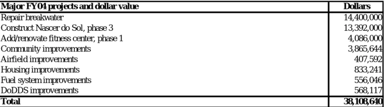
The setup of the policy scenario relies on the evaluation in terms of construction works and repair, employment and private consumption, provided by the U.S. Air Force. The main assumptions are summarized in tables 4 and 5. Table 4 provides an estimation of the losses in terms of construction works and repair caused by the removal of the Lajes Field base, expressed in US dollars.

Table 4: Construction works and repair commissioned by the Lajes Field base

Major FY04 projects and dollar value Dollars

Repair breakwater 14,400,000

Construct Nascer do Sol, phase 3 13,392,000

Add/renovate fitness center, phase 1 4,086,000

Community improvements 3,865,644

Airfield improvements 407,592

Housing improvements 833,241

Fuel system improvements 556,046

DoDDS improvements 568,117

Total 38,108,640

An evaluation of the loss in terms of private consumption, expressed in US dollars, due to the removal of the NATO base is given in table 5. To estimate the local impact on private consumption it has been assumed that 30 per cent of the consumption of active duty personnel living on base originates from the domestic economy. For the active duty personnel living off base the share of private consumption originating from the domestic economy is 50 per cent, while for the US civilians 55 per cent and for the Portuguese civilians 100 per cent.

(26)

Table 5: Estimates regarding the loss in terms of private consumption

Base personnel Annual Payroll ($) Local impact* ($)

Active duty on base 19,814,147 5,944,244

Active duty off base 13,209,431 6,604,716

US civilians 5,163,335 2,839,834

Portuguese civilians 19,322,146 19,322,146

Total impact of annual payroll 57,509,059 34,710,940

Local lodging contracted quarters 1,503

Note: *Estimated pay spent in local economy: 30% of active-duty pay, living on base; 50% of active-duty pay, living off base; 55% civilian pay.

The facility replacement value ($1,075,649,430) has not been taken into account in this policy scenario.

The closing of the Lajes Field base will have direct and indirect impacts on the Azores economy through the following four channels:

The reduction in the demand for construction works and repair;

The employment loss of Portuguese civilians working on the base, which leads to a loss in factor income;

The loss in demand from the US active duty personnel living on base and off base; The loss of rents of local lodging contracted quarters.

The decline in the demand for construction works and repair by the Lajes Field base leads to a decline in investment demand which further affects the production of construction work sector (see table 10). Both profitability and employment in the sector reduce (see tables 11 and 19).

The loss of employment by Portuguese civilians generates a fall in labour income for the Portuguese households. Thus, consumption demand for all products declines (see table 7). Consequently, production of most sectors goes down leading to a downwards adjustment in employment by the sectors.

All these effects are strengthened by the fact that demand from US active duty personnel living on base and off base as well as the US civilians falls. As a consequence, consumption demand for commodities drops by about 2 per cent (see table 7 in the Appendix).

The domestic currency depreciates to maintain the fixed trade deficit thus giving a boost to the external competitiveness by increasing exports to both Mainland and Rest of the World. Therefore, the negative impact induced by the private demand on the production and employment in the agriculture, hunting and forestry sector (sec1), fish (sec2), manufacture products (sec4), transport and communication services (sec9) and financial intermediation services (sec10) is reversed (see tables 10-11). Furthermore, imports from both Mainland and Rest of the World decline due to the relative increase of world prices of imports compared with the domestic prices and the drop in domestic sales. The fall in domestic and foreign savings, i.e. supply of loanable funds, generates a reduction in the demand for investment goods (see table 16).

At the macro level, GDP drops by 0.89 per cent, due to the retrenchment of the private and investment demand. Furthermore, the negative impact on employment accounts for about 0.1 percentage points (see table 6).

(27)

Table 6: Macroeconomic effects (% changes compared with the baseline)

GDP (% change) -0.89

Unemployment rate (%) 4.09

Change in unemployment rate (% points) 1.16

Welfare gains/losses (thousands EURO) -27,919

Welfare gains/losses (% of households income) -2.13

Macroeconomic variables

The measure generates a loss in households’ welfare of about 28 million €, which is equivalent to 2.13 per cent of households’ income.

The detailed sector results on output and prices are depicted in the Appendix.

6. Conclusions

The closure of the Lajes air base does adversely affect the economy. The mechanism is largely driven through the exogenous cut in American expenditure affecting the demand for services, construction and rental housing, besides increase in unemployment on account of job losses. The job loss leads to a fall in income and demand for both domestic and imported commodities forcing the producers to export more to the mainland and ROW.

(28)

References

Armington, P. (1969). A theory of demand for products distinguished by place of production. IMF Staff Papers, 16, 159-178.

Brooke, A., Kendrick, D., Meeraus, A., & Raman, R. (1998). GAMS – A user’s guide. Washington: GAMS Development Corporation.

Harrison, G. W., & Kriström B. (1997). General equilibrium effects of increasing carbon taxes in Sweden. Retrived from: http://www.sekon.slu.se/~bkr/Beijer.pdf.

Löfgren, H., Harris, R. L., & Robinson S. (2002). A standard computable general equilibrium (CGE) in GAMS. IFPRI, Microcomputers in Policy Research, vol.5.

Stone, R. (1954). Linear expenditure systems and demand analysis: An application to the pattern of British demand. Economic Journal, 64, 511-527.

Varian, H.R. (1992). Microeconomic analysis. New York: W.W. Norton.

Dervis, K., De Melo, J., & Robinson, S. (1982). General equilibrium models for development policy. Cambridge, UK: Cambridge University Press.

Sandra Hoffmann, Sherman Robinson, & Shankar Subramanian (1996) The role of defense cuts in the California recession computable general equilibrium models and interstate factor mobility, The Journal of Regional Science, Basil Blackwell, Volume 36 Issue 4 Page 571-595, November 1996

(29)

Appendix

Detailed sector results of the policy measure

Table 7: Changes in private consumption compared with the baseline (%)

Private consumption Commodities % change

Products of agriculture, hunting and forestry sec1 -1.95

Fish sec2 -1.88

Products from mining and quarrying sec3 -2.62

Manufactured products sec4 -2.68

Electrical energy, gas, steam and hot water sec5 -1.51

Contruction work sec6 -2.05

Wholesale and retail trade services; repair services of motor vehicles, motorcycles and personal and

household goods sec7 -2.03

Hotel and restaurant services sec8 -2.71

Transport, storage and communication services sec9 -3.00

Financial intermediation services sec10 -2.73

Real estate, renting and business services sec11 -2.66 Public administration and defence services,

compulsory social security services sec12 -2.36

Education services sec13 -2.37

Health and social services sec14 -2.32

Other community, social and personal services sec15 -2.53 Private household with employed persons sec16 -2.58

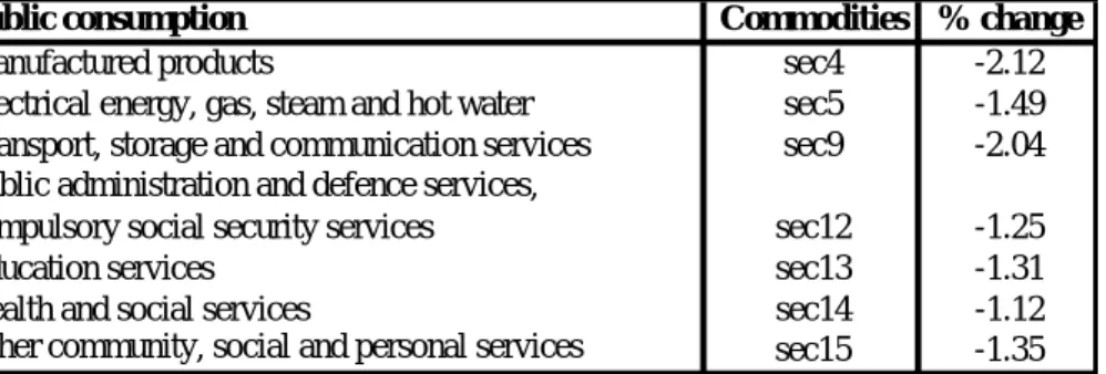
Table 8: Changes in government purchase of goods and services w.r.t. baseline (%)

Public consumption Commodities % change

Manufactured products sec4 -2.12

Electrical energy, gas, steam and hot water sec5 -1.49 Transport, storage and communication services sec9 -2.04 Public administration and defence services,

compulsory social security services sec12 -1.25

Education services sec13 -1.31

Health and social services sec14 -1.12

Other community, social and personal services sec15 -1.35