Taking the pulse of the real economy

(1)

TAKING THE PULSE OF THE REAL ECONOMY

Improving macro forecasts through Alternative Breakdown implementation

and reducing aggregation bias

MASTER THESIS

Date: 4th January 2019

University: Universidade Nova de Lisboa Faculty: School of Business and Economics Department: Finance

Supervisor: Prof. Irem Dermici

Name: Valentin Toshev ID number: 30302

Study: International Finance Specialisation: Corporate Finance

(2)

Abstract

In this research, I show that aggregate information from financial statement analysis helps in predicting real economic development. Further, I show that using the top 100 U.S. public companies, ranked by market capitalisation, represents a convenient method to proxy for the entire portfolio of traded companies. I then show that aggregate accounting information of the same 100 biggest companies has predictive information for next quarter real Gross Domestic Product (GDP) growth, after controlling for the traditional stock market returns, and explains a portion of professional macro forecasters’ revisions and errors. Konchitchki and Patatoukas (2014a) provide an intuitive framework for these findings. Yet, I contribute by finding that aggregate accounting drivers from the Alternative Breakdown provide greater predictive power when compared to DuPont and that introducing financial and nonfinancial data split reduces heterogeneity. Another contribution of mine is introducing out-of-sample analysis. Although, I find that current methods used by professional macro forecasters exhibit slightly lower root-mean-square error (RMSE), I only use annual stock market returns and aggregate accounting profitability drivers in my model.

Keywords: financial statement analysis; accounting; stock valuation; macro forecasting; macroeconomics; aggregate accounting profitability drivers.

(3)

List of Abbreviations

Abbreviation Meaning

13D SEC form for over 5% shares

AB Alternative Breakdown

ATO Asset Turnover

BAT Business Asset Turnover

FSA Financial Statement Analysis

FYR Fiscal-Year-End

IV Independent Variable

OM Operating Margin

PM Profit Margin

Rd Cost of Debt

RMSE Root-mean-square error

ROBA Return on Business Assets

ROE Return on Equity

SE Standard Error

SIC Standard Industrial Classification SME Small and Medium Enterprises SPF Survey of Professional Forecasters VIF Variance Inflation Factor

(6)

1. Introduction

Understanding the direction of an economy is crucial for both public and private decision makers. From employers who set workers’ money compensations and production schedules to macro economists setting federal budgets and forecasting consequent economic growth. Macroeconomics studies the aggregate economic behaviour of a country through examining specific accounts such as inflation, price levels, national income, rate of growth, gross domestic product, and unemployment. The responsible authority in the United States for economy-wide decisions is the Federal Reserve (The Fed). The Fed is accountable for setting monetary policy and keeping the economy either from overheating or triggering growth (Carlin and Soskice, 2015).

In this paper, I further develop the research done by Konchitchki and Patatoukas (2014a) on the link between macroeconomics and financial statement analysis (FSA). The building block of FSA is that companies disclose financial statements in timely fashion, providing accounting information to the general public, thus, reducing noise and information asymmetry among investors. Financial analysis can be conducted by two tools, either ratio analysis or cash flow analysis. In this research, I focus on ratio analysis which examines the relation between different line items in companies’ financial statements. Evaluating current and prior performance based on ratios is often used as a foundation to predict consequent performance on firm level (Penman, 1992; Fairfield et al.,1996; Abarbanell and Bushee, 1997, 1998). The building block in analysing firm’s performance is its own return on equity (ROE). ROE shows the ability of managers to generate returns on the funds provided by firms’ shareholders. An important indication for the company’s health is whether return of equity is in excess of its cost of capital (Palepu et al., 2015). DuPont analysis, invented by DuPont Corporation in 1920, breaks down ROE in three separate components: Profitability, Asset Efficiency, and Financial Leverage. Net income divided by sales yields the profit margin of a company, which measures profitability. Revenue divided by assets shows the asset turnover of a company and is known as asset efficiency. And assets divided by equity results in equity multiplier or as previously defined financial leverage (Palepu et al., 2015). Breaking down ROE in these three components provides analysts with additional information which is the main driver of higher or lower return compared to competitors. High profit margins attract new entrants and lead to mean reversion, asset turnover is unique, therefore more sustainable competitive advantage, and financial leverage gains depend on financing policies. Although, the accounting fundamentals established in

(7)

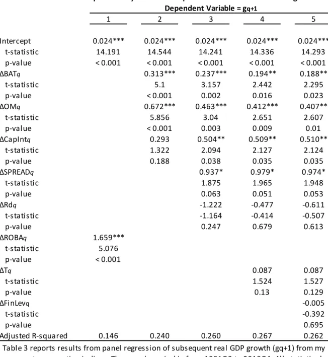
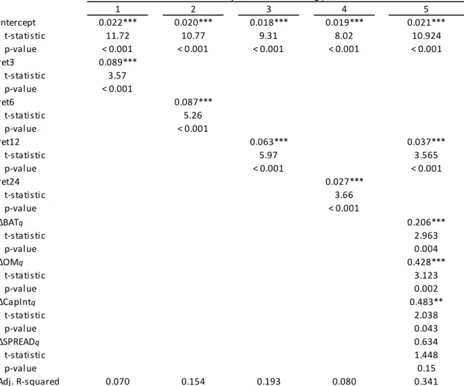
Konchitchki and Patatoukas (2014a) stem from the Classic DuPont breakdown, the two researchers ignore the financial leverage component. The focus of their research is on return on net operating assets (RNOA), and its further breakdown to profit margin and asset turnover (Fairfield and Yohn, 2001; Soliman, 2008). Konchitchki and Patatoukas argue that RNOA offers a more attractive measure at firm level since it is composed from unlevered financial statement items. Nevertheless, understanding whether companies earn returns higher than its cost of capital is crucial. Ivanov (2016) shows that the spread component, which is return on assets minus financing cost, is significant1 and positive predictor for consequent real GDP growth. And the spread component is amplified by the capital structure of the enterprise. Therefore, my first contribution is utilising the Alternative Breakdown (AB) instead of DuPont (Palepu et al., 2015; Ivanov, 2016). AB provides a more thorough perspective because it encompasses return on business assets (ROBA), spread and financial leverage. ROBA measures the efficiency of the company to generate profits by its investment and operating assets scaled by the business assets. Introducing the spread, presents the economic effect of whether the return is enough to cover the borrowing cost. Companies unable to meet their financial obligations have a deteriorating effect on the return on equity. The financial leverage amplifies the positive or negative result by the corresponding liability and equity allocation. To sum up, there are three essential differences between my paper and Konchitchki and Patatoukas (2014a). First, I use ROBA which measures company’s ability to deploy both operating and investment assets, compared to only operating in RNOA. Second, I include spread component, accounting for the incremental usefulness of introducing debt into the capital structure. And third, I control for financial leverage. I conjecture that changes in the Alternative Breakdown ratios have significant relationship with the consequent real GDP growth. Consistent with my conjecture, financial statement analysis performed at aggregate level, provides useful information for consequent economic growth. ΔROBA is a significantly positive independent variable and explains 14.6 percent of the variation in consequent real GDP growth. Decomposing ΔROBA into ΔBAT, ΔOM, and ΔCapInt improves the predictive content to 24.0 percent. Breaking down AB further increases the explanatory power up to 26.7 percent.

Second contribution is introducing data splits by the two sub-hypotheses. The intuitive logic behind this decision stems from sample’s heterogeneity which has been pointed as a driver of insignificant results for some variables (Konchitchki and Patatoukas, 2014a; Ivanov, 2016). I

(8)

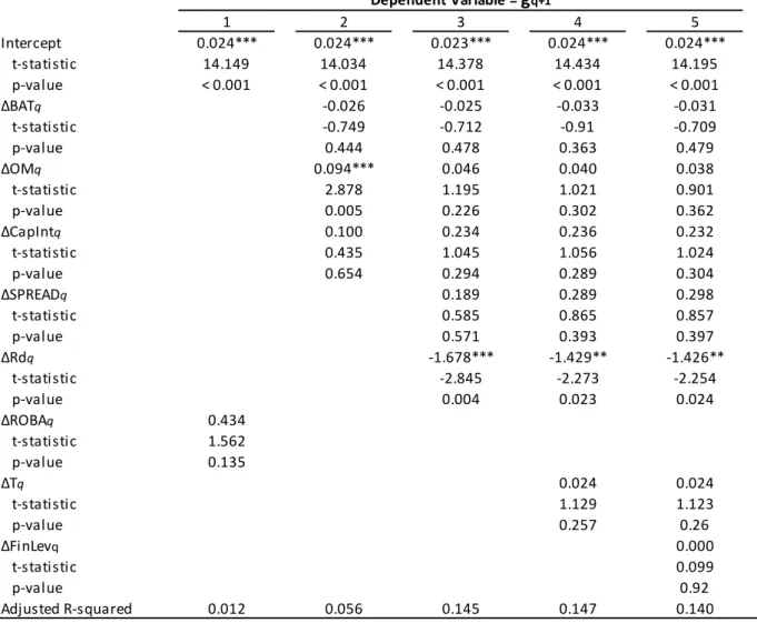
motivate my data separation by the following criteria, previous academic motivation, easiness for implementation and whether at least 100 companies remain in each filter. I first test whether domestic companies provide better proxy for corporate profits’ component of the GDP. Companies operating in the domestic market must pay 100% of their taxes in the U.S. and multinational companies (MNCs) might not. MNCs use a wide range of techniques to pay the least possible taxes through ambiguous transfer prices, company debt location and tax system loopholes. On the contrary to my prediction, the explanatory power of the domestic companies is significantly lower compared to the overall sample. The change in return on business assets of domestic companies explains 6.7 percent of the consequent real GDP variation compared to the 14.6 percent in all companies. Although, the domestic companies exhibit similar increase in explanatory power as all companes, it peaks at 9.7 percent in Column four. There is one apparent limitation in the way I split the data. I use Compustat Domestic and International tickers, which do not allow to examine the percentage of international activity, thus, companies with little to almost none international activity are also dropped.

Most of the empirical literature developed between 1960s and early 2000s has been suggesting that credit growth to the financial industry is contributing to growth boost. On the contrarily, more recent research suggests that high credit to GDP is dampening the economy growth if it is extended to the financial industry. The main reasons behind that are diminishing returns from an increase of the financial industry. The human intensity of the above-mentioned sector, which draws people from R&D and the high capital to income ratios are leading causes (Bezemer et al., 2016; Cecchetti and Kharroubi 2012). Therefore, I conjecture that separating companies in nonfinancial and financial will have a positive impact on the predictive content. Coinciding with my conjecture, changes in the AB ratios of nonfinancial companies predict variations of consequent real GDP growth with higher precision. All columns exhibit higher predictive content, except the first one. Nonfinancial companies’ peak in adjusted R squared is 29.6, compared to 26.7 percent in all companies and 14.7 percent in financial. Furthermore, the independent variables also exhibit higher overall significance level which can be a sign of reduced heterogeneity.

Per Fama (1981; 1990), the stock prices depict the investors’ expectations regarding the future economic development and provide information regarding the consequent economic growth or decline. To address the question, I first examine if the stock markets contain any predicting power for subsequent real GDP growth. The 12-month buy-and-hold returns (ret12) exhibit the highest goodness of fit. In my third contribution, I investigate if the aggregated accounting

(9)

profitability drivers can provide additional forecasting power which is not contained in stock prices. The results, which are based on the AB ratios of nonfinancial companies2, provide incremental explanatory power over consequent real GDP growth, even after controlling for stock market returns. Furthermore, the adjusted R squared increases from 19.3 percent for stock market returns to 34.1 percent when aggregated accounting drivers are included.

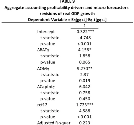
The authority setting interest rate policies in the US is the Federal Reserve. The Federal Reserve uses credible forecast information provided by Survey of Professional Forecasters (SPF), executed by the Federal Reserve Bank of Philadelphia. However, I predict that macro forecasters are unaware of the usefulness of accounting information (Konchitchki and Patatoukas, 2014). Coinciding with my conjecture and marking my fourth contribution, the alternative breakdown and stock market returns explain 22.3 percent of macro forecasters’ revisions. Moreover, forecasting errors of SPF are also predictable through aggregate changes in business asset turnover and stock market returns. Both independent variables explain 6.0 percent of next quarter prediction error. Expanding on the previous results, I test the impact of aggregate accounting drivers on future stock market returns. The aggregated accounting profitability drivers have no explanatory power for the future stock market returns.

In Konchitchki and Patatoukas (2014a), their model provides significant predictability power of consequent real GDP growth and macro forecasters’ errors. Therefore, providing them with a low-cost and efficient model to improve SPF forecasting accuracy. In my fifth contribution, I examine whether the same aggregate accounting profitability drivers can predict the macro forecasters’ revisions after the article has been made available. I run auxiliary tests on the different regressions, which are not presented in the paper, but show that the macro accounting literature had impact on forecasters. However, the post publishing period is rather short, only 25 more observations, therefore, I cannot draw definitive conclusions. In my final contribution, I test the predictive ability of the model in an out-of-sample situation. Comparing to the RMSE of the SPF forecasts, my model has larger errors by 0.23 percent, but the results are promising and provide ground for further research.

The remainder of the paper goes as follows. Section 2 presents prior research in the field of financial statement analysis and connects it to economic growth prediction. In Section 3, I motivate my research hypotheses. Section 4 describes my research design. Section 5 contains

2_{I also ran additional analysis to test if all companies do not provide higher predictive content. The Adjusted}

(10)

empirical results. Section 6 presents out-of-sample comparison to current macro forecasters’ methods. Finally, Section 7 contains concluding remarks, limitations and paths for further research.

(11)

2. Literature Review

The modern society metaphor for King Arthur seeking for the holy grail is the public and private sector’ eagerness to predict economic development. Macroeconomic volatility is significant not only for the development of the gross domestic product but also important in equity market valuation (Aked, Mozzoleni and Shakernia, 2017). The remainder of this section will lead the reader through the development of financial statement analysis and its link to forecasting macroeconomic growth. By examining the prior literature, I interlink this section to the next, where I develop the hypotheses of this research. First, I explain the origin of financial statement analysis and its predictive power for earnings on firm level. Second, I examine the literature on DuPont analysis and the choice of certain ratios. Third, I show the founding papers on macro accounting published by Konchitchki and Patatoukas, where the authors link financial statement analysis and DuPont profitability ratios to forecasting economic development. The purpose of financial statement analysis is to improve comparability between companies and reduce informational asymmetry between stakeholders. The works of Beaver (1968), Ball and Brown (1968) set the foundation of accounting researchers analysing the relation between earnings and security returns. There are several different approaches to earnings forecasting. Starting with Kormendi and Lipe (1987) who decompose the earnings into six components and document diminishing relation between transitory3_{components and stock returns. In 1993, Lev}

and Thiagarajan propose an alternative approach by establishing a set of financial ratios proposed by “experts”4_{and test their correlation with contemporaneous stock returns. In their}

article “Fundamental Information Analysis”, Lev and Thiagarajan identify 12 fundamental signals5 based on practitioners’ toolset when valuing company’s future. Inventory, Receivables, Capital Expenditures, Gross Margin, S&A Expenses, Order Backlog, Labour Force and Effective Tax are significant predictors of excess return variance. Furthermore, Lev and Thiagarajan (1993), find that the fundamental signals can also predict the analysts’ forecast errors. I establish this article as a relevant founding paper to my research since it provides an academic proof of the relationship of the fundamental signals and consequent returns. Abarbanell and Bushee (1997, 1998) further extend the research done by Lev and Thiagarajan (1993) to prove that fundamental analysis can deliver alpha as the market underuses the

3_{Transitionary items refer to items which are further down the balance sheet (Bagnoli and Watts, 2007).}

4_{Which is referred to as guided research, compared to statistical procedure. The difference is that the former uses}

intuitive motivation whereas the latter might identify hard-to-justify balance sheet items.

(12)

available information. Abarbanell and Bushee use the same fundamental signals as defined by Lev and Thiagarajan (1993) and find that analysts misuse fundamental analysis information and their ex post forecast errors are predictable. Abarbanell and Bushee (1998) also examine a holdout sample period which leads to the same conclusions as previous tests. Furthermore, they find that sizeable firms are less exposed to trading influence. Thus, contributing to the decision to use the top 100 U.S. companies ranked by market capitalisation. Followed by Fairfield et al. (1996) who apply different income statement items to predict the return on equity (ROE). Their conclusion is that income statement items are less persistent moving down the profit and loss statement.

Moving further, Nissim and Penman (2001) propose a method to equity valuation by using the DuPont analysis and decomposing the company’s return into return on operating assets (RNOA). The profit margin of a company is a composition of different factors such as first mover advantages, product differentiation, positioning, branding, and uniqueness. Asset Turnover (ATO), on the other hand, is internal measurement as it represents efficiency of a company and asset usage. The nature of the two components is different as high profit margins draw new competition and profits exhibit mean-reversion. On the other hand, production efficiency is harder to imitate. Per prior research, ATO changes provide significant predictive capabilities for subsequent RNOA and are of more persistent nature (Fairfield and Yohn, 2001). Soliman (2008) tries to establish if the DuPont composition retains its persistency when the Fama-French risk factors and Abarbanell and Bushee fundamental signals are included. The risk factors control whether abnormal returns are subject to an increase in company’s exposure. The fundamental signals control whether DuPont analysis provides any incremental predictive power. Since the gross margin (GM) and profit margin (PM) have similar definition, and ATO and CapEx, too. The findings confirm previous research which suggests that level of PM and ATO have insignificant relation with changes in RNOA. On the other hand, changes in ATO explain consequent period’s RNOA variation and retain significance even with the inclusion of fundamental signals and risk-factors. Another compelling evidence is that all fundamental factors from Abarbanell and Bushee retain consistency in terms of magnitude, sign, and significance as per prior research (Abarbanell and Bushee, 1998; Lev and Thiagarajan, 1993). Suggesting that both fundamental signals and DuPont analysis provide explanatory information regarding subsequent period changes in RNOA. The two models are not self-excluding and increase the explanatory power when both of them are included. Changes in ATO is also significant in predicting consequent stock return, analysts forecast revisions and errors withal

(13)

(Soliman, 2008). A limitation of this study is that the author does not include the fundamental signals to control if those do not already predict these forecast errors. Considering that Lev and Thiagarajan (1997) establish a correlation between fundamental signals and forecast errors of analysts6. All in one, the research proves that DuPont analysis is incrementally useful in forecasting consequent profitability. Supplementary to earlier studies, Soliman (2008) examines the behaviour of analysts and stock market investors to understand to what extend they consider PM and ATO when predicting future behaviour of returns. Accordingly, the market recognises RNOA’s significance but does not fully apprehend the magnitude. Therefore, forecasters’ revisions and errors are predictable by changes in ATO.

Expanding previous research and connecting two streams of literature Konchitchki (2013) lays the foundations of the macro accounting. In the paper “Accounting and the Macroeconomy: The Case of Aggregate Price-Level Effects on Individual Stocks” (Konchitchki, 2013) proves that as financial statements are in nominal terms and not inflation adjusted, there are discrepancies in the purchasing power. He provides an example where a company buys land 60 years and 1 year ago for $100 each, adding up to $200 in the financial statement. But under U.S. GAAP only downward revaluation are possible, otherwise the book value is kept at purchase price. Konchitchki (2013) proposes a cost-efficient way by separating accounting information into two components: monetary holdings and nonmonetary holdings. Prior research concludes that on aggregate levels the correlation between inflation and stock returns is negative (Bodie 1976; Fama and Schwert 1977; Fama 1981). During high inflation periods stocks deliver inferior returns and are inadequate hedging technique. Konchitchki (2013) challenges this assumption by developing ex ante strategy based on company-by-company foundations. The method yields significant results and provides a stock-hedging strategy against inflation. Additional contribution to the literature is establishing connection between accounting data on company-level to the forecast of macroeconomic performance. Yet, Konchitchki is using a complex algorithm to adjust for inflation effects. Implementing it at aggregate level is difficult which is limitation of my study as the financial statement items are not inflation adjusted7. Concluding, this article sets the foundation for their further research by demonstrating a correlation between financial statement data and consequent economic realisations.

6_{Abarbanell and Bushee’s fundamental signals are identical to those established in the preceding research done}

by Lev and Thiagarajan.

(14)

Konchitchki and Patatoukas (2014b) argue that using aggregated quarterly data of all listed companies is more consistent approach. The aforementioned articles discuss the informational context of accounting data on firm-level, yet, Konchitchki and Patatoukas (2014b) establish a link between financial statement data and gross domestic product growth. Corporate profits are integral part of GDP, under the income approach, and must exhibit correlation with the other components (Fischer and Merton, 1984; BEA, 2004). Public companies are obliged to report their quarterly earnings compared to the current method implemented by BEA, where corporate profits are forecasted based on IRS’ tax return extrapolation with a two-year lag. Additionally, financial statement analysis is a significant predictor of consequent company performance, therefore, a good proxy for taxes payable by the company. On the other hand, economists consider accounting as non-sense, and do not apply it to their predictions (Konchitchki and Patatoukas 2014b). This is best represented by a quote from McCloskey (1993, p,111): “We economists spurn accounting - another course I never took. But we end up reinventing it. Maybe we should study the subject a little, or at least make our students learn it. After all, it's what we really, truly know.”. And further proven by the lack of references to the topic in the meetings minutes of Federal Open Market Committee. The aggregate accounting earnings prove to be significant and positive over a horizon of up to four quarters. Therefore, it is a clear that aggregate accounting earnings growth have substantial forecasting power regarding the successive GDP growth. Furthermore, the predictive capabilities in one quarter ahead are the strongest, in terms of significance and slope coefficient. Additionally, aggregate accounting earnings growth explains forecasters’ errors in up to three quarters in the future. Again, as with the GDP growth, the most significant is predicting one-quarter-ahead. All in one, Konchitchki and Patatoukas (2014b), prove that aggregate accounting earnings growth has predictive power for up to four quarters but is strongest in the consequent. Furthermore, they prove that macro forecasters do not consider accounting earnings as relevant and that forecast errors can be explained by the data available on company-level. These findings provide foundation for the next paper.

Konchitchki and Patatoukas (2014a) hypothesize that financial statement analysis can be utilised to predict future real economic growth. Widely accepted technique is to use return on net operating assets (RNOA) as an indicator of the company performance8 (Soliman, 2008). Operating income is the difference between sales and cost of goods sold, depreciation expense

8_{The link between previous papers is obvious, by predicting enterprises’ earnings they funnel in the taxable income}

(15)

selling, general, and administrative expense. Net operating assets is operating assets minus non-operating cash and short-term investments, minus non-interest-bearing liabilities. This type of breakdown presents RNOA as an unlevered estimate of company business performance.

𝑅𝑁𝑂𝐴 = 𝑆𝑎𝑙𝑒𝑠

𝑁𝑒𝑡 𝑂𝑝𝑒𝑟𝑎𝑡𝑖𝑛𝑔 𝐴𝑠𝑠𝑒𝑡𝑠 ×

𝑂𝑝𝑒𝑟𝑎𝑡𝑖𝑛𝑔 𝐼𝑛𝑐𝑜𝑚𝑒 𝐴𝑓𝑡𝑒𝑟 𝐷𝑒𝑝𝑟𝑒𝑐𝑖𝑎𝑡𝑖𝑜𝑛

𝑆𝑎𝑙𝑒𝑠

The first component is referred as asset turnover (ATO) and provides an overview of company’s efficiency to generate sales relative to its assets. The second part know as profit margin (PM) determines how well a firm controls its expenses. Konchitchki and Patatoukas (2014a) fill a much-needed gap in research literature by trying to predict overall economic activity by aggregating firm-level data. I contribute to this research by replacing the DuPont analysis with Alternative Breakdown (AB). Consisting of three essential differences, return on equity, role of leverage within a company, and whether a company earns returns higher than cost of debt. I further discuss the reasons for choosing AB in the next chapter. The results show that aggregate accounting profitability drivers, and especially ∆OM and ∆DEP have significant predictive content for consequent real GDP growth. Konchitchki and Patatoukas (2014a) prove a significant importance of accounting data and underutilisation by macro forecasters, but also investors. Yet, some of the variables expected to be significant in the research are not. With a possible explanation being the heterogeneity of the sample. Thus, I include two different splits in my data, the financial to nonfinancial and domestic to MNCs. In the following sections, I back the choices by previous research conducted on the topics.

Equation 1. RNOA decomposition (Konchitchki and Patatoukas, 2014)

(16)

3. Hypothesis Development

3.1. The Alternative Breakdown

The Alternative Breakdown (AB) is a similar decomposition as DuPont analysis with one essential difference, it shows broader range of variables in the decomposition of return on equity. AB provides an overview of company’s activities both on the business and investment side, therefore, supporting a more thorough examination of firm’s performance (Ivanov, 2016; Palepu et al., 2015). In Konchitchki and Patatoukas (2014a), the two researchers only use profitability and asset efficiency perspective of DuPont - return on net operating assets (RNOA). RNOA shows the operating picture of a company, whereas return on business assets (ROBA) also accounts for investment assets. Additionally, the Alternative Breakdown also includes two extra components Spread and Financial Leverage as it can be seen in Equation 2 and also in Appendix 1: Derivations and Ratio list.

𝑅𝑂𝐸 = 𝑅𝑒𝑡𝑢𝑟𝑛 𝑜𝑛 𝐵𝑢𝑠𝑖𝑛𝑒𝑠𝑠 𝐴𝑠𝑠𝑒𝑡𝑠 +

(𝑅𝑒𝑡𝑢𝑟𝑛 𝑜𝑛 𝑏𝑢𝑠𝑖𝑛𝑒𝑠𝑠 𝑎𝑠𝑠𝑒𝑡𝑠 – 𝐼𝑛𝑡𝑒𝑟𝑒𝑠𝑡 𝑒𝑥𝑝𝑒𝑛𝑠𝑒 𝑎𝑓𝑡𝑒𝑟 𝑡𝑎𝑥) × 𝐹𝑖𝑛𝑎𝑛𝑐𝑖𝑎𝑙 𝐿𝑒𝑣𝑒𝑟𝑎𝑔𝑒

When a company finances its activities solely with equity, return on business assets (ROBA), would equal ROE. Return on business assets minus cost of borrowing, referred to as spread, indicates if operating and investment returns are greater than interest cost paid. If a company’s business returns are lower than cost of debt, introducing debt to their financial structure destroys value for equity holders. Furthermore, this economic effect is magnified by debt to equity ratio, referred to as financial leverage in the equation. All in one, a clear predictor of future returns is whether companies deliver higher returns than their cost of debt. Otherwise, companies will either become insolvent or need a major financing restructuring which would have negative implications for consequent period’s GDP growth. Moreover, ROBA can be decomposed into extended DuPont breakdown utilised by Konchitchki and Patatoukas (2014a). Therefore, providing a clear understanding if the additional variables provide any incremental usefulness for prediction next period GDP growth.

𝑅𝑂𝐸 = (1 − 𝑇𝑎𝑥 𝑅𝑎𝑡𝑒) × ((𝑂𝑝𝑒𝑟𝑎𝑡𝑖𝑛𝑔 𝑀𝑎𝑟𝑔𝑖𝑛 𝐵𝑒𝑓𝑜𝑟𝑒 𝐷𝑒𝑝𝑟𝑒𝑐𝑖𝑎𝑡𝑖𝑜𝑛 − 𝐶𝑎𝑝𝑖𝑡𝑎𝑙 𝐼𝑛𝑡𝑒𝑛𝑠𝑖𝑡𝑦) × 𝐵𝑢𝑠𝑖𝑛𝑒𝑠𝑠 𝐴𝑠𝑠𝑒𝑡 𝑇𝑢𝑟𝑛𝑜𝑣𝑒𝑟 − 𝑅𝑑) × 𝐹𝑖𝑛𝑎𝑛𝑐𝑖𝑎𝑙 𝐿𝑒𝑣𝑒𝑟𝑎𝑔𝑒

Equation 2. Classic Alternative Breakdown (Palepu, Healy, and Peek, 2015)

(17)

Each separate variable from the Alternative Breakdown flows differently into the gross domestic product and its consequent growth patterns. Based on the literature review, I expect significant and positive relationship between changes in financial statement items and consequent company growth. Therefore, the same variables should show persistency and significance in predicting consequent GDP growth (Soliman, 2008; Konchitchki and Patatoukas, 2014a, 2014b). Leading to my first and most prominent conjecture.

H1. Fluctuations in aggregate accounting profitability drivers from the Alternative Breakdown can be utilised to predict consequent real GDP growth.

In the following subsubsections I define each variable used as a component of the Alternative Breakdown and conjecture their impact on consequent real GDP growth predictions. The derivation of the Alternative Breakdown and the corresponding components are available in Appendix 1: Derivations and Ratios.

3.1.1. Business Asset Turnover (BAT)

Business Asset Turnover is the ability of a company to generate revenues in relation to business assets (Fairfield and Yohn, 2001). The ratio is referred as asset utilisation and shows how much sales a company makes per dollar of business asset. A change in ATO is linked to improving or deteriorating productivity and is a sound predictor of future profitability. Efficiency materializes from better utilisation of property, plant, and equipment which is difficult to imitate by existing competitors or new entrants. Therefore, the benefits of these changes are less transitory (Soliman, 2008). Furthermore, Romer (1986) proves that changes in capital returns are more persistent predicter of consequent company performance compared to profit margins due to mean reversion and accounting reasons.

Although, previous theoretical works support the hypothesis of ATO being a better predictor, Konchitchki and Patatoukas (2014a) find that on aggregate level asset turnover does not provide useful information regarding consequent GDP growth. There is a twofold explanation for the results. Firstly, heterogeneity of the sample and different asset usage. And secondly, largest companies in the US economy have high efficiency levels with relatively no to infrequent changes in their asset utilization (Ivanov, 2016). Yet, predicting the impact of business asset

Equation 3. Extended Alternative Breakdown Model (Ivanov, 2016)

(18)

turnover is difficult due to the opposite findings of the articles before and after 2014 (Romer, 1986; Fairfield and Yohn, 2001; Konchitchki and Patatoukas, 2014a; Ivanov, 2016).

3.1.2. Capital Intensity

Changes in depreciation are a sound predictor of future economic activity at firm level (Ou and Penman, 1989; Cheng, 2005). In my sample, the top 100 companies are ranked by market capitalisation, but most of them are also leaders based on physical assets, too (Murphy, 2018). Therefore, depreciation expense is substantial, and large changes can be related to replacement or enhancement of existing assets. The purchases represent large investments and can be expected to have positive link to real GDP growth. Company acquisitions of new assets funnel into the income approach twice – firstly, new machines are either more efficient or provide greater capacity and secondly, it is a corporate sale for another company.

On the other hand, real earnings management (REM) cuts in selling, general and administrative expenses and consequent reversals are a significant predictor of lower future performance (Vorst, 2015). If the management manages earnings with an objective to meet earnings benchmarks, issuance of debt or equity, or achieving compensation thresholds, their consequent performance will be damaged. In the light of Vorst (2015), a decrease in new asset investments compared to their competitors can lead to lower future efficiency and profitability. Hence, sacrificing company’s competitive position in the market and potentially leading to bankruptcy. Yet, this effect can be muted on aggregate level and large U.S. companies are thoroughly followed by analysts, leaving less room for earnings manipulation by management. In Konchitchki and Patatoukas (2014a), changes in depreciation exhibits significant and positive relationship. I conjecture that in my findings the results are also significant and with positive sign.

3.1.3. Tax Rate

In the income approach to measure GDP, corporate profits are a main driver. Therefore, using the extended AB in which the effective tax rate is calculated, should yield significant correlation with the consequent GDP growth (Konchitchki and Patatoukas, 2014b). The effective tax rate is a better predictor compared to statutory rates since it incorporates tax reliefs and benefits. Referring to Appendix 3, where all twelve variables from Lev and Thiagarajan (1993) are explained, an increase in effective tax rate provides only transitionary benefits. The impact of

(19)

increased company net earnings and decreased effective tax rate9 has a negative effect on corporate profits component of GDP. On the other hand, due to the transitionary nature of these changes, Lev and Thiagarajan (1993) conjecture that a decrease in effective tax rate will have positive effect on GDP growth when a reversal occurs. However, increased effective tax rate will result in more corporate profits which drive GDP growth and increased effective tax rate depresses nominal growth based on Keynesian tax theory (Furceri and Karras, 2011; Ivanov, 2016). Additionally, tax smoothing theory suggests that companies issue debt during recession with repayment schedule in expansion (Barro, 1979). Therefore, I conjecture that the impact of tax rate is ambiguous as an increase in tax rate will mean more income from taxes for the government, but also reduce the willingness of companies to produce.

3.1.4. Financial Leverage

The debt and equity composition of companies has been extensively discussed in theory of Modigliani-Miller (1959). Under certain set of key assumptions10_{the framework hypotheses}

that firm value is only determined by its earnings power and is not dependent on financing decisions. In the described environment, returns only switch from equity to debt holders and vice versa. I will not examine in-depth the best aggregate capital structure strategy due to sample’s heterogeneity which is translated into different per sectors optimal capital structures. For example, utility companies have steady cash-flows allowing them to take on greater debt. Additionally, in the sample there are both financial and nonfinancial firms which highly differ in their capital structure. Loans are liabilities for the latter companies, but assets for the banking industry. Furthermore, under the Basel III regulators have imposed non-risk leverage ratio restrictions which limits the financial exposure (Smith, Grill and Lang, 2017). An undeniable benefit for increasing debt is the tax shield, however, very high leverage ratio can trigger covenants and destabilise the company further resulting in higher financing costs.

On the other hand, Karpavicius (2014) proposes an alternative argumentation suggesting a significant relationship between optimality theory and capital structure. By modifying the sample to account for behavioural biases, namely the short-term outlook of management, also discussed previously under Vorst (2015). Under favourable market conditions high levels of debt can be sustainable, refinancing risk low and threat of triggering covenants insignificant. Nonetheless, financial difficulty can prompt banks to downsize loans based on asymmetric

9_{Without the respective increase in statutory tax rate. Analysts consider such decrease transitionary (Wall Street}

Journal, 1990).

10_{Such as no taxes, no bankruptcy costs, symmetry of market information, no transaction costs, equal borrowing}

(20)

information also damaging healthy companies. From the financial perspective of the sample, in time of crisis, the interbank markets experience considerable pressures and pose a liquidity pressure to serve its existing obligations to companies (Allen and Carletti, 2008).

Furthermore, the equity holders, as residual claimants, can be viewed to hold a long call with strike price of the liabilities value. Therefore, they only make money if the assets are worth more than the debt.

[Insert Figure 2 here]

Viewing the company from this perspective, we can use Black-Scholes option pricing model to determine the call value. Establishing that debt holders have a fixed pay-out and the excess is claimed by equity holder brings conflicting interests. Considering two alternative projects, equal investment value, yet Project A is riskier than Project B. The latter project has larger variance, higher payoff in the up state (favourable) and lower payoff in the down state

(bankruptcy). Therefore, shareholders’ decision favours the riskier project since in down state

the company is bankrupt, and their payoff is zero but have a higher upside (Amaro de Matos, 2008).

Moreover, shareholders have voting majority and can exert power over the direction of a company, thus, shareholder activism becomes a threat for the optimal capital structure. Furthermore, Klein and Zur (2011) find evidence that shareholder activism reduces bond holders’ wealth. Hedge fund activism results in excess return of -3.9 percent in the day before and after the 13D filing, and -4.5 percent in the following year subsequent of the filling date. Targeted companies decrease their cash at hand, double common shareholder dividends and increase debt-to-asset ratio. Thus, companies face prospective interest and principal payments with depleted cash accounts, resulting in credit risk increase. Hence, leading to substantial amount of companies being downgraded after the initial 13D filing. These finding are not contradictory to earlier positive abnormal returns attributed to shareholder, but rather to wealth expropriation from debt to equity holders (Klein and Zur, 2011).

All in one, increased debt can be beneficial for a company in terms of tax benefits, but this can also be caused by shareholder activism raising company’s volatility and overall risk. Therefore, the relationship between GDP growth and companies’ leverage is ambiguous at aggregate level. Not in terms of the weight attributable to changes in debt level, but the causality of this variation is unknown.

(21)

3.1.5. Cost of Debt

A conventional method to estimate the cost of debt is through defaultable bond pricing. Investors in corporate bonds suffer an extra risk of the company going bankrupt, thus, demand a higher return. Figure 3 represents a usual connotation of such formula, where YTMC and

YTMG are yield to maturity of a corporate bond and government bond with identical maturity,

and GSPREAD is an additional yield investor requires for the extra risk. Although, there are more

sophisticated methodologies11, this model provides the basic option pricing foundation (Pereira, 2018).

𝑌𝑇𝑀𝑐 = 𝑌𝑇𝑀𝐺 + 𝐺𝑆𝑃𝑅𝐸𝐴𝐷

YTMG is a proxy for the risk-free rate set by the Central Bank and is an essential tool of

monetary policy kit to regulate inflation levels. Under the three-equation model of macroeconomic policy, proposed by Carlin and Soskice (2015), an increase in policy rate is to tackle inflationary shocks. Therefore, an increase in risk-free is related to a decrease in consequent period economic output and results in lower GDP growth. On the other hand, if the change in cost of debt is only due to increased risk of a company12, I expect the effect on real GDP growth to be insignificant. On an occasion that the change is on aggregate level, decreased cost of debt can be perceived as lower risk economic risk. To understand better if cost of debt fluctuations are due to the policy rate or mark-up, the analysis must evaluate the companies on firm-level. Yet, the purpose of this study is to use aggregate changes.

All in one, the cost of debt fluctuations provide ambiguous relationship to the consequent real GDP growth as they can be of double nature. Increasing the risk-free rate is a tool used by the Central Banks, to contract the economy. On the other hand, aggregate risk premium increase can also have a negative impact on the economy because investors predict greater risk for which they must be compensated.

3.2. Domestic Sales

The published research by Konchitchki and Patatoukas (2014a, 2014b), provides findings that aggregate accounting earnings variation is a significant predictor about the future GDP. As

11_{For example, interest swap rate interpolation, option adjusted spread and risk-neutral pricing model} 12_{I assume the risk-free remains unchanged and the change is only in the mark-up}

(22)

previously discussed in Section 2 Literature Review, accounting earnings are better predictor for current taxable income than the annual tabulations of IRS.

A critique to the income approach is provided by Viet (2009) in her book for the United Nations Statistics Division. The argumentation behind is that operating surplus can be calculated only for an enterprise and not for its belonging establishments. An example would make it clearer: we have a corporation with three locations, two of which are subsidiaries which produce and sell items and the last one is the headquarter. The operating surplus derivation can be done only on aggregate level and not separately per location. Thus, the consolidated corporate profit cannot be separated for multinational corporations (MNCs) which operate in multiple countries. In this line of thinking Grubert (2012) provides information that from 1996 to 2004, the unrepatriated foreign income13_{rose from 17.4 percent to 31.4 percent. Furthermore,}

investments abroad also rose significantly. Redirecting money outside U.S. through tax differentials by which companies shift income to lower tax places through manipulating the transfer price, company debt location, and other loopholes in the tax systems.

Including home sales of the company, which is an indicator in Bloomberg Professional, will be a good predictor of consequent GDP growth. The main reason is that aggregate accounting is used as a proxy for corporate profits in U.S., but international activities are going to be taxed abroad and only the subsidiaries’ dividends are taxed under American laws (Grubert, 2012). However, including the Bloomberg Professional indicator provides information for only 10 years behind and proved hard to use on aggregate level. Therefore, I use the Compustat Domestic and International variables to determine the nature of their operation.

H1a. Changes in aggregate accounting profitability drivers of the Domestic Companies provide larger predictive content over consequent real GDP growth in comparison to the whole sample.

3.3. Financial and Non-Financial Breakdown

Most of the empirical literature developed between 1960s and early 2000s suggests that credit growth to the financial industry is contributing to positive economic activity. Rajan & Zingales (1998) provide empirical evidence that industries dependent on external funding exhibit higher growth rates in more financially developed countries. Since financial development decreases

13_{The definition used of foreign income in the paper is subsidiaries’ before foreign tax income of U.S. parent}

(23)

cost of raising funds, reduces asymmetrical information and moral hazards (Greenwood & Jovanovic, 1990).

On the contrarily, more recent research suggests that high credit to GDP is dampening the economic growth if it is extended to the financial industry. The main reasons behind that are the financial industry exhibits diminishing returns and its high human intensity which draws people from R&D positions, potentially impeding the growth of science breakthroughs (Bezemer et al., 2016; Cecchetti & Kharroubi 2012).

Thus, the USA, with its well-developed financial industry and high credit to GDP ratio, will exhibit relatively no correlation to consequent GDP growth.

Furthermore, Konchitchki and Patatoukas (2014a) suggest that their research can be improved by separating the data and further segmenting the sample. I assume that the biggest difference would come from financial and non-financial companies due to their difference in accounting of assets and liabilities (Pariente, 2018). In banks, earning assets represent loans extended to companies, whereas this is liabilities for a non-financial company (Pariente, 2018)

H1b. Changes in the aggregated accounting profitability drivers of the Nonfinancial Companies provide larger predictive content over consequent real GDP growth compared to financial companies and overall sample

3.4. The Stock Market Variable

In the context of rational expectations, we would suppose that stock market investors have anticipated future economic activity, and this is represented in stock prices. Per Fama (1981; 1990), stock prices depict investors’ expectations regarding future economic development and provide information regarding the consequent economic growth or decline. Rational investors are comparable to macro forecasters as they use their knowledge to predict future economic activity (Konchitchki & Patatoukas, 2014a).

Previous empirical research identifies S&P 500 as a suitable proxy for the U.S. market due to its easiness to obtain and interpretation (Konchitchki & Patatoukas, 2014a). Furthermore, S&P 500 is also used as a benchmark to active investing funds, but also replicated by passive investment funds. Therefore, changes in the index have significant effects on the economy since it is comprised of the top 500 public companies in the U.S.

H2. Aggregated accounting profitability drivers are beneficial in macro forecasting and are not subsumed by stock market returns

(24)

To address the question, I first examine if stock markets contain any predicting power for subsequent real GDP growth. Afterwards, I investigate if aggregate accounting profitability drivers can provide additional forecasting power which is not contained in stock prices.

3.5. History of Macro-Forecasting

The Federal Reserve administers the interest rate policies in the US. In targeting equilibrium output the Federal Reserve gathers its information from the Survey of Professional Forecasters (SPF) which is executed by the Federal Reserve Bank of Philadelphia. As the oldest and most reputable source of quarterly macro forecasts, SPF has a network of financial professionals, academia, government, labour unions and trade associations who provide quarterly predictions. Given that reputation is an important factor for those individuals and institution, they have an intrinsic incentive to provide accurate forecasts. The survey focuses on 27 different variables, weighting on mainly CPI inflation, GDP growth, and yields on long-term T-bonds. Therefore, macro forecasters should consider all available information to them at the time of their predictions. I test whether the AB ratios on aggregate level predict the macro forecasters’ revisions from q-1 to q. Consequently, I test if their forecast errors are predictable by the same aggregate accounting information.

Provided that aggregate accounting profitability drivers are not subsumed by stock investors, Konchitchki and Patatoukas (2014a) conjecture that macro forecasters are also unaware of the informative power of DuPont analysis. As in “Accounting earnings and gross domestic product”, the two researchers use SPF consensus forecasts as a proxy for the assumptions made by the U.S. Federal Budget (Konchitchki and Patatoukas, 2014a, 2014b). Since Federal Reserve’s Board of Governors utilises the SPF forecasts in the preparation of the “Greenbook” prior to the Federal Open Market Committee, Sims (2002) discovers that Greenbook predictions are identical to the SPF panellists as both groups’ reputation and jobs are at stake.

Broadening previous results that DuPont ratios on firm-level predict analysts’ forecast errors and on aggregate level DuPont explains variation in macro forecast errors (Soliman, 2008; Konchitchki and Patatoukas, 2014a). I predict that macro forecasters do not fully utilise the information in the financial statements of companies, in particular the AB ratios. Since, economists consider accounting as irrelevant to their work and lacks any useful information for their forecasts.

H3. Whether the macro forecasters (SPF) embed aggregate accounting profitability drivers from the alternative breakdown when forming their revisions of real GDP growth

(25)

H4. Whether SPF forecast errors are predictable by aggregate accounting profitability drivers from the alternative breakdown and stock market returns

3.6. Stock Valuation

Previous research provides evidence for the significant importance of the macroeconomic fluctuations in stock valuation. An important relation was established among stock pricing and its corresponding firm fundamentals with the inclusion of inflation and real GDP variables. Whether macro variables are included, fundamental factors results were insignificant (Lev & Thiagarajan, 1993). As discussed in the financial literature, the firm-level delay in accounting data assimilation provides the investors with an opportunity to earn abnormal returns (Abarbanell & Bushee, 1998; Soliman, 2008). If the model developed using accounting drivers can predict future real GDP growth and improve macro forecasters’ accuracy, I expect that stock market prices are not immediately affected but with a lag14.

H5. How do accounting profitability drivers affect the stock valuations based on the real GDP information provided?

14_{I structured my report in a way that cornerstone articles are examined in detail in section 2. Allowing me to}

briefly summarize the paragraph leading to the research questions. The main reason behind that is readers with satisfactory knowledge on the topic can benefit from easier composition and time-saving.

(26)

4. Methodology

4.1. Sample

I retrieve quarterly income statement and balance sheet data from Compustat Quarterly Preliminary History Dataset. The focus is only on companies which fiscal quarter ends align with calendar quarter ends - March, June, September, and December. I calculate quarterly ratios changes of profitability which are composed by ROBA15_{, Financial Leverage, and Cost of Debt.}

To tackle any data seasonality, I multiply all income statement variables by four. Consequently, I use year-over-year changes when compiling quarterly profitability ratios16. Furthermore, I eliminate companies which lack information for ratio calculation. To mitigate for the outlier’s effects, I exclude the top and bottom one percent of each profitability driver. Companies with negative Cost of Debt are also excluded from the sample17.

I retrieve SPF data from the Federal Reserve Bank of Philadelphia18 with a date span of 1981Q3 to 2018Q1, with only one missing data for the period of 1995Q4. The missing data point happened as a result of a governmental shutdown because of budgetary reform conflict. There are two reasons for the beginning point of my sample period to be 1981Q3. Firstly, Compustat data is limited beforehand. And secondly, SPF’s reports have been delivered in a consistent manner only after 1981Q3. I source the data on GDP preliminary growth from National Income and Product Accounts (NIPA) which is governed by the Bureau of Economic Analysis (BEA). I collect GDP growth forecast data of the mean19 SPF consensus for consecutive quarter q+1 denoted Eq[gq+1]. I use S&P 500 as a proxy for stock market portfolio and measure this by the

equites market return of a buy-and-hold portfolio with holding period of 3, 6, 12, and 24 months. Once, I have all the necessary data, I calculate each ratio for companies which have FYR as calendar quarters using Excel. In Stata, I filter the data to top 100 enterprises by market capitalisation, aggregate the ratios quarterly, and compute the changes from the same quarter, but the previous year. Second, I test if segregating the data to companies operating solely in the home market (U.S.) and multinational companies provide different predictive power. I filter by

15_{As previously discussed in Section 2.4. ROBA differentiates slightly from RNOA presented in the Konchitchki}

and Patatoukas (2014a).

16_{Konchitchki and Patatoukas (2014a, 2014b) use this method, moreover, Fairfield (2001) proves its effectiveness}

to tackle biasness by annualizing data.

17_{This is not a representation of survivorship bias, but rather safeguarding my data from outliers. It seems}

unreasonable to assume that a company would receive money for taking a loan.

18_{The Federal Reserve Bank of Philadelphia started facilitating the Survey of Professional Forecasters since 1990.} 19_{I obtain the mean consensus forecast of the SPF analysts compared to the individual predictions which are}

(27)

Compustat domestic and international indicators. The filtering of the data is easily done by introducing an if test or simple dummy variable. Consequently, I implement an identical process as with the data for all companies. Third, previous research suggests that financial sector expansion has diminishing contributions to economic growth. Thus, I conjecture that, a well-developed financial sector as in U.S., will explain smaller variation of consequent GDP and nonfinancial enterprises’ predictive content will raise since heterogeneity will be reduced. I use the SIC codes and separate the dataset in financial industry 6000-6799 and the rest which I refer to as nonfinancial industries. The rest of remaining procedures are duplicated as per Hypothesis 1. Fourth, if the initial hypothesis is proven, next step will be to include stock market return in macro forecasting models. This would determine if the information provided in AB ratios is not already included in stock market return. Konchitchki and Patatoukas (2014a), find that the greatest predicting power for consequent quarter is provided by the returns in previous 12 months20_{. Therefore, it suggests that investors’ forecasts of economic development is strongest}

at one year horizon. Hypothesis 2 examines the relationship between the 12 months buy-and-hold returns and test whether the aggregate ratios provide additional information. Expanding on the previous regressions, it would be useful to test whether forecast errors of SPF forecasters can be predicted by stock market returns and aggregate profitability drivers. Predicting that macro forecasters do not utilise accounting data due to being “too coarse” will be proven if any

β is significant. The concluding test examines whether the stock participants utilise the

accounting information in their prediction of the future stock market returns. The final model conjectures whether the future S&P returns can be predicted by the fitted value of real GDP growth (ĝ) based on the AB ratios, yet not already subsumed by the returns from the previous year (ret12). I use only the significant independent variables from Table 6 which are ΔBAT, ΔOM, ΔCapInt, and ΔSPREAD, to predict ĝ. I follow by estimating residuals and regressing them on future returns.

4.2. Timing of the experiment

The main reason to align fiscal and calendar quarters is to match the timing of SPF. The Federal Reserve Bank of Philadelphia sends the questionnaires to macro forecasters within one month after each quarter ends. Therefore, companies without financial statement data available by the end of first month (t) after fiscal quarter (q) are excluded from the sample. Using this method

20_{I also test if this is the case in my dataset by regressing consequent real GDP growth by 3, 6, 12, and 24 month}

returns. As per Konchitchki and Patatoukas (2014a), I find that the 12 month return has the highest predictive ability.

(28)

assures that all information is available to macro forecasters ex-ante. To align the financial information, I use conditional formatting provided by Compustat and fix the Fiscal-Year-End (FYR) to 3, 6, 9, and 12. Figure 4 illustrates the process and research design timeline, providing an example for 2011 (Konchitchki & Patatoukas, 2014a). SPF sends the questionnaires by the end of July 2011, thus financial statements information released by that time is readily available for their analysis. Analysts must deliver their prediction by the middle of next month. In Figure 4 macro forecasters receive prediction questionnaires by the end of July 2011 and return them by middle of August 2011.

[Insert Figure 4 here]

4.3. Descriptive statistics

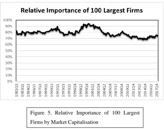
Figure 5 shows the top 100 U.S. firms, ranked by market capitalisation, as a fraction from the total market with aligning fiscal and calendar quarters. During the sample period, I find that my sample accounts for 79% on average of the population. However, in recent years we can see that line hoovers closer to 70% rather than 80%. Benjamin Graham, the father of value investing, provides a good explanation for this phenomenon. In the rise of a bull market, investors focus their money in fewer, bigger companies. But if the upward trend persists, smaller and mid-size companies exhibit interesting returns, too. Luring investors to spread their funds among more companies. Evidence points to a conclusion that positive returns in the SMEs are mainly driven by speculation. This explanation fits in the current state of the economy, where stocks exhibit all time high, therefore high market capitalisation is not clustered to few large companies (Graham, 2003).

(29)

Next, I present the descriptive statistics in Table 1 and the pairwise correlations in Table 2. The first noticeable divergence in the descriptive statistics of Konchitchki and Patatoukas (2014a) and mine are between values of assets turnover and return on assets. This can be explained as Konchitchki and Patatoukas (2014a) calculate those ratios based on the net operating assets where I use business assets which include also investment assets. Thus, the denominator of ROBA ratio is expected to be larger. Profit and Operating margins are very close to the original paper, but as expected 43 basis and 160 basis points higher, respectively. This can be explained as in the calculation of those ratios I include the investment profits as well. The cost of debt is between 54 and 250 basis points which can be attributable to the size of the companies, but also the monetary policies. The mean effective tax rate of the sample is 32 percent which is very close to the statutory tax rate21.

21_{Although the statutory tax rate was changed to 21 percent in the end of 2017 by the Tax Cuts and Jobs Act}

(TCJA), the effect can be observed only in 2018Q1 which is not enough to drive the mean downwards (Congress, 2017).

Figure 5. Relative Importance of 100 Largest Firms by Market Capitalisation

(30)

Although Ivanov (2016) ranks companies based on their assets, the mean, min, and max values of the variables are very close to each other. Understandably, the biggest companies in terms of assets and market capitalisation are not identical, but similar (Murphy, 2018). This serves as a good check due to the similarity of the ratio definition.

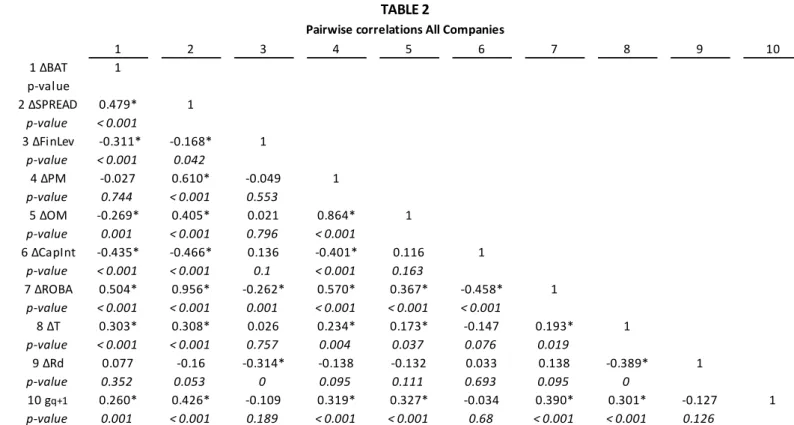
Second, pairwise correlations are presented in Table 2. The table already hints which variables will have a predictive power over consequent GDP growth. Yet, I test their combined significance in the following section. The correlation matrix also brings the multicollinearity problem as cost of debt is correlated to the financial leverage and tax rates. Therefore, in the following regressions I compute multicollinearity diagnostics, yielding very low Variance Inflation Factor (VIF) in all test regressions and proving no multicollinearity signals. I also check whether the results are different when excluding the cost of debt, financial leverage, and

Variable Mean Std.Dev. Min Max

BAT 0.34 0.051 0.218 0.456 SPREAD 0.023 0.008 0.005 0.038 FinLev 0.91 0.215 0.493 1.453 PM 0.174 0.029 0.115 0.227 OM 0.249 0.03 0.173 0.303 CapInt 0.075 0.009 0.049 0.104 ROBA 0.035 0.005 0.022 0.049 Rd 0.012 0.004 0.005 0.025 T 0.32 0.054 0.143 0.44 BAT -0.007 0.03 -0.104 0.083 SPREAD 0 0.005 -0.023 0.022 ΔFinLev 0.013 0.15 -0.464 0.393 ΔPM 0.002 0.016 -0.055 0.058 ΔOM 0.003 0.015 -0.043 0.045 ΔCapInt 0.001 0.008 -0.025 0.021 ΔRd 0 0.002 -0.005 0.007 ΔROBA 0 0.005 -0.024 0.022 ΔT -0.006 0.034 -0.095 0.093 gq+1 0.024 0.023 -0.061 0.087

Table 1 reports descriptive statistics for the quarterly time-series of the following aggregate ratios: BAT, SPREAD, FinLev, OM, PM, CapInt, Rd, T, and ROBA. Aggregate year-over-year changes are represented by Δ symbol. The sample period is from 1981Q3 to

2018Q1. *All numbers are presented in decimals

Descriptive Statistics

(31)

tax rates, the results yielded negligible differences in the overall predictive content and independent variable wise. As expected, some of the other variables exhibit correlation since they represent parts of the decomposed ratios. The changes in BAT, SPREAD, PM, OM, ROBA, and T, as shown in the last line of Table 2, show correlation at the 5 percent significance level.

4.4. Additional tests

I briefly go through few of the additional tests I ran to confirm that the correlation between variables in the descriptive statistics is not affecting the following regressions. I estimate the regressions in Section 5: Results using ordinary least squares regressions, I further perform standard errors Newey and West (1987) test with lag length of 4. I find no autocorrelation beyond four quarters behind. Assuring that the standard errors (SEs) are robust is important, otherwise, it can lead to incorrect rejection or acceptance of null hypothesis, Type I error. All regressions have robust SEs and exhibit no systematic pattern in residuals22.

22_{I also double check the results through using vce (robust) function in Stata.}

1 2 3 4 5 6 7 8 9 10 1 ΔBAT 1 p-value 2 ΔSPREAD 0.479* 1 p-value < 0.001 3 ΔFinLev -0.311* -0.168* 1 p-value < 0.001 0.042 4 ΔPM -0.027 0.610* -0.049 1 p-value 0.744 < 0.001 0.553 5 ΔOM -0.269* 0.405* 0.021 0.864* 1 p-value 0.001 < 0.001 0.796 < 0.001 6 ΔCapInt -0.435* -0.466* 0.136 -0.401* 0.116 1 p-value < 0.001 < 0.001 0.1 < 0.001 0.163 7 ΔROBA 0.504* 0.956* -0.262* 0.570* 0.367* -0.458* 1 p-value < 0.001 < 0.001 0.001 < 0.001 < 0.001 < 0.001 8 ΔT 0.303* 0.308* 0.026 0.234* 0.173* -0.147 0.193* 1 p-value < 0.001 < 0.001 0.757 0.004 0.037 0.076 0.019 9 ΔRd 0.077 -0.16 -0.314* -0.138 -0.132 0.033 0.138 -0.389* 1 p-value 0.352 0.053 0 0.095 0.111 0.693 0.095 0 10 gq+1 0.260* 0.426* -0.109 0.319* 0.327* -0.034 0.390* 0.301* -0.127 1 p-value 0.001 < 0.001 0.189 < 0.001 < 0.001 0.68 < 0.001 < 0.001 0.126

* shows significance at the .05 level

Table 2 reports Pearson correlation and two-sided p-values in italics. The sample period is from 1981Q3 to 2018Q1. Pairwise correlations All Companies

(32)

Moving our attention to the multicollinearity threat. Having a high correlation between independent variables can lead to large standard errors, which in turn will damage the representativeness of the current sample. Since some of the variables are defined as composite measures, they can be representative of perfect multicollinearity (Allen, 1997). Therefore, I exclude the ΔROBA after the first column and ΔRd which proves to be insignificant in the first regression, as those two variables are used to construct ΔSPREAD. Although perfect multicollinearity presents a threat, the solution is rather simple by excluding the composite measure or the constructing variables (Allen, 1997). I also test for extreme multicollinearity, to determine if the independent variables are exhibiting any signs. Allen (1997) suggests that multicollinearity can also be detected by examining the magnitude of the coefficients and standard deviations of the regressors. However, the VIF test suggests that there is no multicollinearity between the variables23_{. As Ivanov (2016) argues in his research, the}

insignificant relationship between the variables can be due to the heterogeneity of the sample, company specifics also affect the capital structure, and prior research focuses on long-term effects compared to my short-term horizon.