Study of the Drying Kinetics of Pears from cultivar D. Joaquina

(1)

Study of the Drying Kinetics of Pears from cultivar

D. Joaquina

Raquel P. F. Guiné1and Maria João Barroca2

1_{CI&DETS/ESAV, Instituto Politécnico de Viseu, Portugal (e-mail: raquelguine@esav.ipv.pt).}

2_{CERNAS/ISEC, Instituto Politécnico de Coimbra, Portugal (e-mail: mjbarroca@gmail.com).}

Conference Topic –CT4 – Bioengineering and Biotechnology Abstract

Drying is one of the most widely used methods for preserving foods allowing extending their shelf life by minimizing the moisture content in the food so that the deterioration reactions will not be able to occur.

The objective of the present work was to determine the drying kinetics of pears from cultivar D. Joaquina, and then use the experimental data to model the drying kinetics by means of different thin layer equations found in the literature. For that two temperatures were tested (60 and 70 ºC) and seven models were analysed.

The results obtained allowed concluding that while some models were very adequate to predict the drying behaviour like Newton, Page, Modified Page, Henderson & Pabis and Logarithmic, others were not so good, such as Wang & Singh and Vega-Lemus.

Key Words: Pear, Drying, Kinetic model, Thin layer model.

1. Introduction

The pear (Pyruscommunis L.) is original from temperate zones such as Europe, being cultivated in several countries, including Portugal. Their flavour is influenced by the volatile aromatic compounds present and by the ratio between the contents of sugars and organic acids, such as citric and malic acids, which are the predominant acids present. The pH stands in the range 2.6-5.4, and its bitter taste is normally associated with the rind, due to the phenolic and polyphenolic compounds. The colour of the peel depends on the amount and type of pigments present, being mainly chlorophyll (green) and carotenoids (yellow) [1], [2]. Drying of food products was one of the first preservations techniques used and is still nowadays a very important method of preservation which can be applied to a wide range of products[3], [4].

Drying has e primal role in the food processing industries [5], and is one of the most widely used methods for preserving foods [6], which allows extending their shelf life by removing the water to a level that minimizes the deterioration phenomena due to microorganisms, enzymes or ferments [7]–[9]. Besides preservation, other advantages of drying include lighter weight for transportation and smaller space needed for storage, as well as avoiding the need of expensive refrigeration systems, with obvious economic benefits [6], [9], [10].

The project and construction of drying systems is frequently done empirically, based on the extrapolation of knowledge existing for other cases. However, reliable process modelling is based on the knowledge about the physico-chemical behaviour of the foods, and also the drying kinetics, which accounts for the mechanisms of water removal [1], [11], [12].

The dehydration of hygroscopic food products is very complex being further difficult by their complex internal structure. Many studies have been conducted on the moisture transfer phenomenon, for many different food products and considering different types of kinetics. In scientific literature are described many different kinetic models, either mechanistic, empirical, or a combination of both [12]–[15].

The present work aimed at determining the drying kinetics of pears from cultivar D. Joaquina, as described by empirical models cited in the literature, for the convective drying performed at different temperatures.

(2)

2. Experimental

Pears of the variety D. Joaquina were used in this study. The pears of this variety are very sweet and quite small (about 4 to 5 cm diameter maximum) and exhibit good drying features [1]. The pears were dried in a drying chamber with ventilation (model WTB from Binder, Germany) at constant temperature, but with trials done at different temperatures. The air

flow was 300 m3_{/h and the air circulated parallel to the samples, at 0.35 m/s. The inlet}

average temperature was constant in each experiment, and experiments were conducted at different temperatures of 60 and 70 ºC, until they reached a moisture content of less than 1%, so as to obtain a highly crispy product.

Periodically samples were removed randomly in order to measure their average water content. The measurements were made with a Halogen Moisture Analyser (model HG53, from Mettler Toledo, USA), which was previously calibrated in terms of optimal operating parameters for this type of food. The operating conditions used were: temperature of 120 ºC, speed 3 = medium (in a scale of 1 = very fast to 5 = very slow).

3. Mathematical Modelling

Simulation models are basilar for the design of new driers or for the improvement of existing drying systems, besides being of extreme importance for the control of the drying operations. The drying kinetics may be fully described through the transport properties of both the material and the drying medium. In the drying of food products, it is typically used the drying constant, K, which combines all the transport properties and may be defined by the thin layer equation [4], [16].Thin layer equations are equations aimed to describe the drying phenomena in a combined way, despite of the controlling mechanism, and have been used to estimate drying times for several products and to access drying curves. Several thin layer equations, varying widely in nature, are available in the literature and have been used by many investigators to successfully explain the drying of several agricultural products [16], [17].

The drying kinetics was monitored in terms of evolution of the moisture content along drying, and the data was then expressed in terms of the dimensionless variable moisture ratio, defined as:

MR = _WW - We

0 - We (1)

where W is the moisture content at time t, W0 is the initial moisture content and We is the equilibrium moisture content, all expressed in dry basis.

To model the drying kinetics the experimental points (MR, t) were fitted to different empirical kinetic models from literature as shown in Table 1[10], [16], [18].

Table 1 – Empirical models to represent the drying kinetics.

Model name Equation

Newton MR = exp(- k t)

Page MR = exp(- k tn₎

Modified Page MR = exp(- (k t)n₎

Henderson & Pabis MR = a exp(- k t)

Logarithmic MR = a exp(- k t) + c

Wang & Singh MR = 1 + a t + b t2

Vega-Lemus MR = (a + k t)2

It is worth emphasize that the models used to describe the drying kinetics are empirical and therefore do not necessarily have a phenomenological meaning. They are merely equations that have been found to adequately represent the experimental data obtained for the drying curves.

(3)

The fittings were obtained with software SigmaPlot V11.0 (Systat Software, Inc.). To evaluate the most appropriate model to describe the drying behavior of the D. Joaquina pears, some statistical indicators were used as described by the following equations[4], [13], [19]–[25]:

Mean absolute error:

∑

=

−

=

N i

V

i

V

predi

N

MAE

1 exp, ,

1

(2)

Root mean square error:

∑

=

−

=

N i

V

i

V

predi

N

RMSE

1 2 , exp,

)

(

1

(3) Standard error:

1 )

(

1 2 , exp,

−

=

∑

₌

N

V

SE

N i i predi (4)

Sum of square errors:

∑

=

−

=

N i

V

i

V

predi

N

SSE

1 2 , exp,

)

(

1

(5) Chi square:

∑

=

−

=

N i i predi p

V

n

N

CS

1 2 , exp,

)

(

1

(6)

Relative percent deviation:

∑

=

−

=

N i i i pred i

V

N

RPD

1 exp, , exp,

100

(7)

In the above equations N is the number of observations and np is the number of parameters,

while Vexp,i and Vpred,i are the experimental and predicted values for the dependent variable at

any observation i. RMSE and CS aim at comparing the differences between the experimental and predicted values, and when they approach zero it indicates that the prediction is closer to the experimental data [22], [23]. On the other hand, the relative percent error compares the absolute differences between those values, and for RPD under 10 % the fit is considered to be good [23]. RMSE provides information on the short-term performance of the correlations by allowing a term by term comparison of the actual deviation between the calculated value and the measured value [10]. Other statistical information provided is the number of observations, correlation coefficient and standard error of estimate. Furthermore, an analysis of variance was also included, providing information about the F-test and the P-value. High values of F-test indicate the suitability of the models to describe the experimental data [21]. Other statistic testes used were the normality test (Shapiro-Wilk), the W Statistic and the constant variance test.

4. Results and Discussion

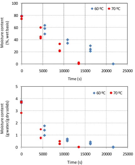
Figure 1 shows the evolution of the moisture content of D. Joaquina pears along drying, as expressed in wet basis and also in dry basis, for the two temperatures studied. The results show that in some cases for the same time the results of the determinations are slightly different, which is expected given the nature of products being dried, since the biological materials have some differences among the same lot that could account for the differences. However, and not devaluing the previously mentioned reasons, it is believed that the major factor responsible for these differences would be the size of the elements, because even though they were selected as to be the most similar as possible, the true is that a slight difference in the thickness of the sample would result in an additional resistance offered to the moisture diffusion, and therefore it would be expected a slower drying rate. As to the time required to complete the drying process, so as to reach a moisture content under 1% (wet basis), because it was aimed at obtaining a very crispy product, it was observed that the drying time was 6 hoursor3 hours and 45 minutes, respectively for 60 and 70 ºC.

Tables 2 to 9 show the results of the modelling of the drying data for both temperatures studied, with the seven different models tested, whose equations are presented in Table 1. The results indicate that in general all models tested are relatively good to fit the experimental data for both temperatures. However, it is possible to verify that the models with the least good performance were Wang & Singh and Vega-Lemus.

(4)

Figure 1 – Variation of moisture along drying: top - wet basis moisture content, bottom - dry basis moisture content.

Table 2 – Results of the fitting to the Newton Model.

60 ºC 70 ºC

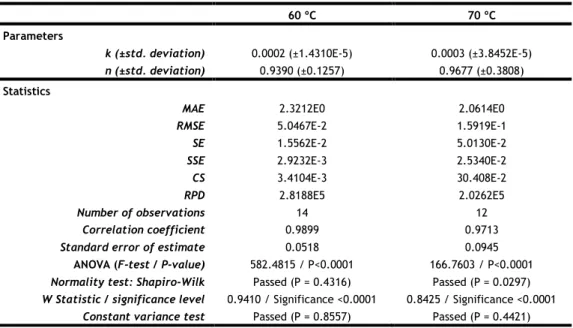
Parameters

k (±std. deviation) 0.0002 (±1.2112E-5) 0.0003 (±3.9677E-5)

Statistics

MAE 4.3521E-2 8.3726E-2

RMSE 5.6965E-2 1.5968E-1

SE 1.6396E-2 5.0285E-2

SSE 3.2450E-3 2.5497E-2

CS 3.4946E-3 2.7815E-2

RPD 9.3840E2 9.2031E2

Number of observations 14 12

Correlation coefficient 0.9896 0.9713

Standard error of estimate 0.0524 0.0946

ANOVA (F-test / P-value) 570.6087 / P<0.0001 166.6622 / P<0.0001

Normality test: Shapiro-Wilk Passed(P = 0.2143) Passed(P = 0.0332)

W Statistic / significance level 0.9192 / Significance<0.0001 0.8464 / Significance<0.0001

Constant variance test Passed (P = 0.7155) Passed (P = 0.2335)

0 20 40 60 80 100 0 5000 10000 15000 20000 25000 M o is tu re c o n te n t (% , w e t b a si s) Time (s) 60 ºC 70 ºC 0 1 2 3 4 5 0 5000 10000 15000 20000 25000 M o is tu re c o n te n t (g w a te r/ g d ry s o lid s) Time (s) 60 ºC 70 ºC

(5)

The results in Table 2 show that the Newton model is very adequate to model the drying kinetics, given the high values of F (∼570 and ∼167 for 60 and 70 ºC, respectively). Also the correlation coefficient is very close to 1 in both cases (0.9896 and 0.9713 for both temperatures). Since the RMSE and CS values, that compare the differences between the experimental data and the predictions given by the model, are in both cases very low, approaching zero, this is indicative that the prediction is very much close the experimental data.

Table 3 – Results of the fitting to the Page Model.

60 ºC 70 ºC

Parameters

k (±std. deviation) 0.0003 (±3.2452E-5) 0.0004 (±0.0001)

n (±std. deviation) 0.9391 (±0.1258) 0.9684 (±0.3811)

Statistics

MAE 3.5060E-2 8.4436E-2

RMSE 4.7991E-2 1.5992E-1

SE 1.3813E-2 5.0363E-2

SSE 2.3032E-3 2.5576E-2

CS 2.6870E-3 3.0691E-2

RPD 2.0701E3 9.6843E2

Normality test: Shapiro-Wilk Passed (P = 0.4314) Passed (P = 0.0297)

W Statistic / significance level 0.9410 / Significance <0.0001 0.8426 / Significance <0.0001

Tables 3 and 4 show that the Page and the Modified Page models are very similar, with values for the parameters k and n practically equal for both temperatures studied. Furthermore, the statistical information also confirms that these two models are adequate to fit the experimental data.

Table 4 – Results of the fitting to the Modified Page Model.

60 ºC 70 ºC

Parameters

n (±std. deviation) 0.9390 (±0.1257) 0.9677 (±0.3808)

Statistics

MAE 2.3212E0 2.0614E0

RMSE 5.0467E-2 1.5919E-1

SE 1.5562E-2 5.0130E-2

SSE 2.9232E-3 2.5340E-2

CS 3.4104E-3 30.408E-2

RPD 2.8188E5 2.0262E5

(6)

Table 5 reveals the results for the Henderson & Pabis model, one of the best given the statistical information that characterizes the fit. In this case the values of F are very high (∼580 and ∼230 for 60 and 70 ºC).

Table 5 – Results of the fitting to the Henderson & Pabis Model.

60 ºC 70 ºC

Parameters

a (±std. deviation) 1.0164 (±0.0362) 0.9112 (±0.0466)

Statistics

MAE 4.2778E-2 9.4407E-2

RMSE 5.5312E-2 1.4471E-1

SE 1.5920E-2 4.5571E-2

SSE 3.0594E-3 2.0941E-2

CS 3.5693E-3 2.5129E-2

RPD 9.5355E2 8.4155E2

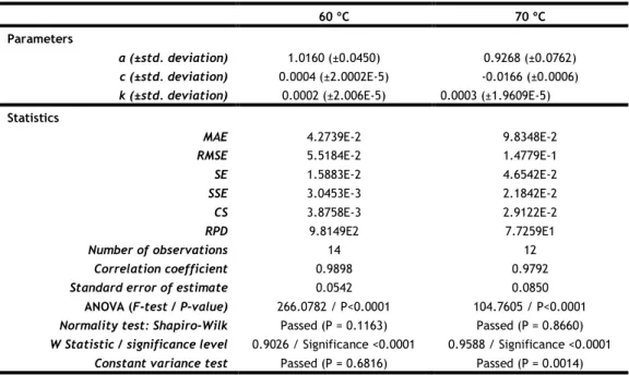
The results for the Logarithmic model shown in Table 6 also reveal that this equation is good to predict the behaviour of the pears at drying. In all cases the values of the standard error associated to estimation of the parameters in the model are under 10 % of the value, thus indicating the accuracy of the estimate.

Table 6 – Results of the fitting to the Logarithmic Model.

60 ºC 70 ºC

Parameters

a (±std. deviation) 1.0160 (±0.0450) 0.9268 (±0.0762)

c (±std. deviation) 0.0004 (±2.0002E-5) -0.0166 (±0.0006)

Statistics

MAE 4.2739E-2 9.8348E-2

RMSE 5.5184E-2 1.4779E-1

SE 1.5883E-2 4.6542E-2

SSE 3.0453E-3 2.1842E-2

CS 3.8758E-3 2.9122E-2

RPD 9.8149E2 7.7259E1

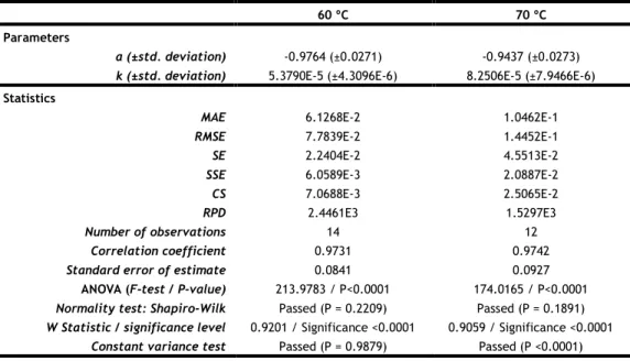
Tables 7 and 8 show the fits for the models Wang & Singh and Vega-Lemus. As it can be seen, these two models, although not totally inadequate, re slightly worse for the description of the kinetics of the D. Joaquina pears, when compared to the other models previously analysed. In fact, the different statistical parameters calculated show this less affinity to the

(7)

experimental data. This conclusion can also be confirmed by visualization of the predictions in the graphical mode.

Table 7 – Results of the fitting to the Wang & Singh Model.

60 ºC 70 ºC

Parameters

a (±std. deviation) -0.0001 (±7.4200E-6) -0.0002 (±1.6113E-5)

b (±std. deviation) 3.1580E-9 (±3.8460E-10) 8.2899E-9 (±1.3534E-9)

Statistics

MAE 1.7223E-1 1.7791E-1

RMSE 2.0356E-1 2.2642E-1

SE 5.8590E-2 7.1304E-2

SSE 4.1439E-2 5.1267E-2

CS 4.8345E-2 6.1520E-2

RPD 2.2310E4 9.9632E3

Table 8 – Results of the fitting to the Vega-Lemus Model.

60 ºC 70 ºC

Parameters

a (±std. deviation) -0.9764 (±0.0271) -0.9437 (±0.0273)

k (±std. deviation) 5.3790E-5 (±4.3096E-6) 8.2506E-5 (±7.9466E-6)

Statistics

MAE 6.1268E-2 1.0462E-1

RMSE 7.7839E-2 1.4452E-1

SE 2.2404E-2 4.5513E-2

SSE 6.0589E-3 2.0887E-2

CS 7.0688E-3 2.5065E-2

RPD 2.4461E3 1.5297E3

Constant variance test Passed (P = 0.9879) Passed (P <0.0001)

Figure 2 shows the fits obtained with two models, one considered as very adequate (Henderson & Pabis, for example) together with one model considered less adequate (Wang & Singh, for example). The graph in the right reveals that the curves are more distant from the experimental points when compared to the curves in the graph on the left.

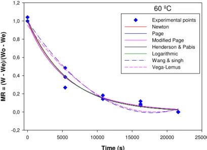
Figure 3 shows for one experimental essay, say for example at 60 ºC, the experimental points as well as the fits obtained with all the models tested in this study, for better visualization of

(8)

the adequacy. The results clearly indicate two categories of models, very similar among each category. The first corresponds to the models that are considered very adequate (Newton, Page, Modified Page, Henderson & Pabis and Logarithmic) and the second corresponds to the less adequate models (Wang & Singh and Vega-Lemus).

Figure 2 – Experimental points and fits obtained with Henderson & Pabis model (left) and Wang & Singh (right).

Figure 3 – Experimental points and fits for 60 ºC obtained with all models tested.

5. Conclusions

From the results obtained it was possible to conclude that although all models tested to describe the drying kinetics of D. Joaquina pears at 60 and 70 ºC showed some degree of adequacy, in fact five of them were highlighted as very good (Newton, Page, Modified Page, Henderson & Pabis and Logarithmic) whereas two others were good at predicting the experimental behaviour of the pears (Wang & Singh and Vega-Lemus).

Acknowledgement

The authors thank FCT (Fundação para a Ciência e Tecnologia) and research centre CI&DETS and CERNAS for financial support.

References

60 ºC Time (s) 0 5000 10000 15000 20000 25000 M R = ( W W e )/ (W o W e ) -0,2 0,0 0,2 0,4 0,6 0,8 1,0 1,2 Experimental points Newton Page Modified Page Henderson & Pabis Logarithmic Wang & singh Vega-Lemus Henderson & Pabis

Time (s) 0 5000 10000 15000 20000 25000 M R = ( W W e )/ (W o W e ) 0,0 0,2 0,4 0,6 0,8 1,0 1,2 60 ºC 70 ºC Fit 60 ºC Fit 70 ºC

Wang & Singh

Time (s) 0 5000 10000 15000 20000 25000 M R = ( W W e )/ (W o W e ) -0,2 0,0 0,2 0,4 0,6 0,8 1,0 1,2 60 ºC 70 ºC Fit 60 ºC Fit 70 ºC

(9)

[1] R. P. F. Guiné, D. M. S. Ferreira, M. J. Barroca, and F. M. Gonçalves, “Study of the drying kinetics of solar-dried pears,” Biosystems Engineering, vol. 98, no. 4, pp. 422– 429, Dezembro 2007.

[2] K. J. Park, A. Bin, F. P. Reis Brod, and T. H. K. Brandini Park, “Osmotic dehydration

kinetics of pear D’anjou (Pyrus communis L.),” Journal of Food Engineering, vol. 52, no. 3, pp. 293–298, May 2002.

[3] R. P. F. Guiné and J. A. A. M. Castro, “Pear Drying Process Analysis: Drying Rates and

Evolution of Water and Sugar Concentrations in Space and Time,” Drying Technology, vol. 20, no. 7, pp. 1515–1526, 2002.

[4] İ. T. Toğrul and D. Pehlivan, “Modelling of drying kinetics of single apricot,” Journal of

Food Engineering, vol. 58, no. 1, pp. 23–32, Jun. 2003.

[5] M. K. Krokida, V. T. Karathanos, Z. B. Maroulis, and D. Marinos-Kouris, “Drying kinetics

of some vegetables,” Journal of Food Engineering, vol. 59, no. 4, pp. 391–403, Oct. 2003.

[6] İ. Doymaz, “The kinetics of forced convective air-drying of pumpkin slices,” Journal of

Food Engineering, vol. 79, no. 1, pp. 243–248, Mar. 2007.

[7] I. Alibas, “Microwave, air and combined microwave–air-drying parameters of pumpkin

slices,” LWT - Food Science and Technology, vol. 40, no. 8, pp. 1445–1451, Oct. 2007.

[8] R. P. F. Guiné, D. M. S. Ferreira, M. J. Barroca, and F. M. Gonçalves, “Study of the Solar

Drying of Pears,” International Journal of Fruit Science, vol. 7, no. 2, pp. 101–118, 2007.

[9] K. Sacilik, “Effect of drying methods on thin-layer drying characteristics of hull-less

seed pumpkin (Cucurbita pepo L.),” Journal of Food Engineering, vol. 79, no. 1, pp. 23– 30, Mar. 2007.

[10] R. Guiné, “Analysis of the drying kinetics of S. Bartolomeu pears for different drying systems.,” EJournal of Environmental, Agricultural and Food Chemistry, vol. 9, no. 11, pp. 1772–1783, 2010.

[11] C. T. Kiranoudis, E. Tsami, and Z. B. Maroulis, “Microwave Vacuum Drying Kinetics of Some Fruits,” Drying Technology, vol. 15, no. 10, pp. 2421–2440, 1997.

[12] M. A. Salgado, A. Lebert, H. S. Garcia, J. Muchnik, and J. J. Bimbenet, “Development of the characteristic drying curve for cassava chips in monolayer.,” Drying Tecnology, vol. 12, no. 3, pp. 685–696.

[13] R. P. F. Guiné and R. M. C. Fernandes, “Analysis of the drying kinetics of chestnuts,” Journal of Food Engineering, vol. 76, no. 3, pp. 460–467, Outubro 2006.

[14] D.-W. Sun and J. L. Woods, “Simulation of the Heat and Moisture Transfer Process During Drying in Deep Grain Beds,” Drying Technology, vol. 15, no. 10, pp. 2479–2492, 1997.

[15] G. Vázquez, F. Chenlo, R. Moreira, and E. Cruz, “Grape Drying in a Pilot Plant With a Heat Pump,” Drying Technology, vol. 15, no. 3–4, pp. 899–920, 1997.

[16] R. P. F. Guiné, P. Lopes, M. Barroca, and D. M. S. Ferreira, “Effect of ripening stage on the solar drying kinetics and properties of s. Bartolomeu pears (Pyrus communis L.),” International Journal of Academic Research, vol. 1, no. 1, pp. 46–52, Sep. 2009.

[17] B. Nourhène, K. Mohammed, and K. Nabil, “Experimental and mathematical investigations of convective solar drying of four varieties of olive leaves,” Food and Bioproducts Processing, vol. 86, no. 3, pp. 176–184, Sep. 2008.

[18] R. Baini and T. A. G. Langrish, “Choosing an appropriate drying model for intermittent and continuous drying of bananas,” Journal of Food Engineering, vol. 79, no. 1, pp. 330– 343, Mar. 2007.

[19] O. Yaldýz and C. Ertekýn, “Thin Layer Solar Drying of Some Vegetables,” Drying Technology, vol. 19, no. 3–4, pp. 583–597, 2001.

[20] M. Al-Harahsheh, A. H. Al-Muhtaseb, and T. R. A. Magee, “Microwave drying kinetics of tomato pomace: Effect of osmotic dehydration,” Chemical Engineering and Processing: Process Intensification, vol. 48, no. 1, pp. 524–531, Jan. 2009.

[21] C. L. Mota, C. Luciano, A. Dias, M. J. Barroca, and R. P. F. Guiné, “Convective drying of onion: Kinetics and nutritional evaluation,” Food and Bioproducts Processing, vol. 88, no. 2–3, pp. 115–123, Jun. 2010.

[22] J. H. Lee and H. J. Kim, “Vacuum drying kinetics of Asian white radish (Raphanus sativus L.) slices,” LWT - Food Science and Technology, vol. 42, no. 1, pp. 180–186, Jan. 2009.

(10)

[23] J. S. Roberts, D. R. Kidd, and O. Padilla-Zakour, “Drying kinetics of grape seeds,” Journal of Food Engineering, vol. 89, no. 4, pp. 460–465, Dec. 2008.

[24] P. P. Tripathy and Subodh Kumar, “A methodology for determination of temperature dependent mass transfer coefficients from drying kinetics: application to solar drying.,” Journal of Food Engineering, vol. 90, no. 2, pp. 212–218, 2009.

[25] A. Vega-Gálvez, A. Andrés, E. Gonzalez, E. Notte-Cuello, M. Chacana, and R. Lemus-Mondaca, “Mathematical modelling on the drying process of yellow squat lobster (Cervimunida jhoni) fishery waste for animal feed,” Animal Feed Science and Technology, vol. 151, no. 3–4, pp. 268–279, May 2009.