The Cold Dark Matter Model with Cosmological Constant and the Flatness Constraint
A.C.B. Antunes∗
Instituto de F´ısica, Universidade Federal do Rio de Janeiro C.P. 68528, Ilha do Fund˜ao, 21945-970 Rio de Janeiro, RJ, Brazil
L.J. Antunes†
Instituto de Engenharia Nuclear - CNEN C.P. 68550, Ilha do Fund˜ao, 21945-970 Rio de Janeiro, RJ, Brazil
(Received on 29 January, 2009)
The Hubble parameter, a function of the cosmological redshift, is derived from the Friedmann-Robertson-Walker equation. The three physical parametersH0,Ω0mandΩΛare determined fitting the Hubble parameter to the data from measurements of redshift and luminosity distances of type-Ia supernovae. The best fit is not consistent with the flatness constraint (k=0). On the other hand, the flatness constraint is imposed on the Hubble parameter and the physical parameters used are the published values of the standard model of cosmology. The result is shown to be inconsistent with the data from type-Ia supernovae.
Keywords: Cold dark matter model, Hubble parameter.
1. THE HUBBLE PARAMETER FROM THE FRIEDMANN EQUATION
From Einstein’s equations for the gravitational field in the Robertson-Walker metric, one can derive the Friedmann dif-ferential equation
˙ R2 c2R2+
k R2−
Λ 3 =
8πGρm
3c2 (1)
and the acceleration equation
¨ R2 c2R=−
4πG 3c2
ρm+3p
c2
+1
3Λ (2)
whereRis the scale factor, kis the curvature index andΛ the cosmological constant. The pressure p is related to the matter densityρmby an equation of state,
p=w c2ρm, (3)
withw=0 for non-relativistic matter [1–4]. Using the vacuum energy density
ρΛ=c2Λ/8πG, (4) and introducing the Hubble parameter
H(R) =R˙
R, (5)
the Friedmann equation reads :
H2(R) +c
2k R2 =
8πG
3 (ρm+ρΛ). (6)
The scale factorRand the matter densityρmare related to their present day valuesR0andρ0mby
ρmR3=ρ0mR03. (7)
∗Electronic address:[email protected]
†Electronic address:[email protected]
Defining an adimensional variable, the cosmological fre-quency redshift,
x=R0
R =1+z, (8)
wherezis the redshift, the equation above becomes
H2(x) +c
2k R20 x
2=8πG 3 ρ0mx
3+ρ
Λ. (9)
For current values, corresponding tox=1, this equation gives
c2k R20 =
8πG
3 (ρ0m+ρΛ−ρc), (10)
whereρc= 3H02/8πGis the critical density andH0is the Hubble constant.
Now the Hubble parameter can be written explicitly as
H2(x) =8πG
3
ρΛ−(ρ0m+ρΛ−ρc)x2+ρ0mx3. (11) Introducing the relative densitiesΩ0m=ρ0m/ρc andΩΛ=
ρΛ/ρc, the Hubble parameter reads
H2(x) =H02ΩΛ−(Ω0m+ΩΛ−1)x2+Ω0mx3
. (12)
The function containing the curvature index and the present day scale factor becomes
c2k R20 =H
2
0(Ω0m+ΩΛ−1). (13)
The acceleration equation
¨ R R=−
4πG 3
ρm+3p
c2
+c
2Λ
3 (14)
can be rewritten as
¨ R R=H
2 0
ΩΛ−1
2
Ω0mx3+ 3p c2ρc
The left-hand side can be written in terms ofx=R0/Rand H(R) =R˙/R. Using
R d dR H
2=−xd dx H
2 (16)
in
¨ R R=H
2(R) +R 2
d dR H
2(R), (17) we obtain
¨ R R=H
2(x)
−x
2 d dxH
2(x)
. (18)
Performing the calculation of the right-hand side with
H2(x) =H02ΩΛ−(Ω0m+ΩΛ−1)x2+Ω0mx3 (19) and equating to the above expression for ¨R/R containing
(3p/c2ρc)we obtainp=0. Thus, the acceleration equation is finally reduced to
¨ R R=H
2 0
ΩΛ−
1 2Ω0mx
3
. (20)
This result permits to obtain the value ofxat the equilib-rium point corresponding to ¨R=0:
xe= (2ΩΛ/Ω0m)1/3. (21) The dimensionless deceleration parameter
q=−R˙R¨
R2 =− ¨ R
RH2 (22)
can be calculated at the present day condition (x=1): q0=−
1 H2
0
R¨
R
0
=−
ΩΛ−1
2Ω0m
(23)
The age of the universe (t0) can be obtained from the Hub-ble parameter
H(R) =R˙
R=− 1 x
dx
dt , (24)
then
t0= Z ∞
1 dx
x H(x). (25)
With the above expression forH2(x)we have H0t0=
Z ∞
1
dx
xpΩΛ−(Ω0m+ΩΛ−1)x2+Ω0mx3 (26)
1.1. Determination of the parameters by fitting H(x) to type-Ia supernovae data
LetHe0= 65 km·s−1·Mpc−1be a nominal value of the Hub-ble constant; defining the function
y(x) =H
2(x)
e
H02 , (27)
with
y0= H2
0
e
H02, (28)
and also the parameters
a1=y0ΩΛ, a2=−y0(Ω0m+ΩΛ−1) and a3=y0Ω0m, (29) the above equation for the Hubble parameter gives
y(x) =a1+a2x2+a3x3. (30) The three parameters of this polynomial function can be de-termined by fitting data from measurements of the luminosity distances and the redshift of the type-Ia supernovae. These parameters and their sum,y0=a1+a2+a3, give the physical parameters
Ω0m=
a3 y0
, ΩΛ=
a1 y0
, and H0=He0√y0. (31) To fit the Hubble parameter to the data from redshift(z)
and luminosity distances (D) measurements of type-Ia super-novae, some changes of variables are in order. The published data set is[5]
{zj, vj=log(czj), uj=log(H0e Dj), σuj ; j=1, ..,N},
with N=230 .
The Hubble parameter is
H(x) = (c z/D). (32)
As
y(x) =H(x)/He0
2
=c z/He0D
2
, (33)
and
log(y(x)) =2[log(c z)−log(He0D)] =2(v−u), (34) then
y(x) =102(v−u). (35) The data set to be used in the fitting is
{xj,yj,σj;j=1, ..,n} which is obtained from the first set using
xj=1+zi , yj=102(vj−uj) , and σj=2.ln10.yjσuj. (36) Details of the fitting are presented in the appendix. The results of the fitting give the following values for the physical parameters:
H0 = (60.2±0.4)km.s−1.Mpc−1 (37)
Ω0m = 0.26±0.04 (38)
ΩΛ = 1.55±0.11 (39)
and the age of the universe
t0= (30.0±1.3)×109 yr . (41) The point of null acceleration is
xe=
2 ΩΛ Ωom
1/3
=2.28 (42)
which corresponds to the redshift
ze=1.28 (43)
2. THE FLATNESS CONSTRAINT
The cosmic microwave background (CMB) observations suggest that the spacial geometry of the Universe is very close to flat. According to equation (13) the zero curvature corresponds to the conditionΩom+ΩΛ=1. If this condition is imposed on the Hubble parameter (see equation (12)), we have
H2(x) =H02ΩΛ+Ω0mx3, (44) with
ΩΛ=1−Ω0m. (45)
The polynomial form, equation (26), becomes
y(x) =a1+a3x3 (46) where y(x) =H(x)/He0
2
, a1=y0ΩΛ, a3=y0Ω0m and
y0=
H0/He0
2 .
The accepted values for the physical parameters of the cold dark matter model with cosmological constant (ΛCDM) subjected to the flatness constraint (k=0) are [6]:
H0=71±4 km.s−1.Mpc−1 and ΩΛ=0.73±0.004 . (47) So, the coefficients of the polynomial in equation (32) are a1=0.87 anda3=0.32. The deceleration parameter is
q0=−1
2(3ΩΛ−1) =−0.6 , (48)
and the point of null acceleration is
xe=
2ΩΛ
Ω0m
1/3
=1.8 , (49)
corresponding to the redshiftze=0.8 . The age of the Uni-verse is
t0=13.7 Gyr . (50)
The sum of the weighted square deviations for this model, as defined in the appendix, is
χ2=16780.10 . (51)
3. CONCLUSION
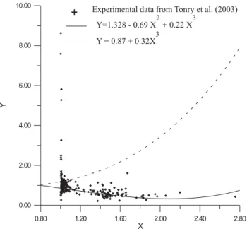
The cold dark matter model with cosmological constant (ΛCDM) is expressed by the Hubble parameter as a function of the cosmological redshiftx=1+z. This function is de-rived from the Friedmann equation in the Robertson-Walker metric. The square of the Hubble parameter is an incomplete third-degree polynomial function in the variablex=1+z. This polynomial is least-squares fitted to data from the mea-surements of the redshifts and luminosity distances of the type-Ia supernovae, and the three non-null coefficients of the polynomial and the uncertainties and covariances are then computed. The physical parameters are obtained from the three non-null coefficients, showing that these supernovae data are sufficient to determineH0,Ω0m andΩΛ, the three fundamental parameters of the ΛCDM model. The results of this model are compared with the published results of the ΛCDMmodel with the flatness constraint (k=0)[6](see Fig. 1).
In this second model, theΛCDM (k=0), the measure-ments from the cosmic microwave background (CMB) are also taken into account. The results of these models dis-agree. TheΛCDM model fitted to the Ia supernovae data implies a positive curvature index (k= +1) and a large age for the Universe. This conflicts with the results of the CMB measurements. On the other hand, theΛCDM(k=0) model presents large deviations from the type-Ia supernovae data. Both models are consistent with the evidences of an ac-celerating expansion of the Universe [7–11]. However, in any way there are clear disagreements between models and data. Some observable measurements are model-dependent. These observables are related to the parameters of the model. The values of the parameters must be fixed so that these ob-servables can be computed from other observable measure-ments.
Thus, it is a contradictory result that theΛCDM (k=0) model, which is used in the computation of the luminosity distances of these Ia supernovae, be in disaccord with these same data.
Appendix A
In this appendix we collect some formulas used in the fit-ting of the polynomial function
f(x;a1,a2,a3) = a1f1(x) +a2f2(x) +a3f3(x), withf1(x) = 1 ,
f2(x) = x2, andf3(x) =x3, (52) to the data set
{xj,yj,σj;j=1, ..,n} (53) obtained from the published data[5] by the transformations
0.80 1.20 1.60 2.00 2.40 2.80
X
0.00 2.00 4.00 6.00 8.00 10.00
Y
Y = 0.87 + 0.32X3
Experimental data from Tonry et al. (2003)
Y=1.328 - 0.69 X + 0.22 X2 3
FIG. 1: A plot of the functiony(x) = (H(x)/He0)2for two models: the best fit for theΛCDMmodel withk= +1 (continuous line) and theΛCDMwithk=0 with the published values[6] for the physical parameters (dashed line). For comparison, the experimental points corresponding to{xj,yj}[5] are also depicted.
The least-squares method is used to determine the parameters a1,a2anda3which minimize the function
χ2(a1,a2,a3) =
N
∑
j=1pj[yj−f(xj;a1,a2,a3) ]2 , where pj= 1 σj
.
(55) The minimum condition
∂χ2
∂aj
=0 (j=1,2,3) (56)
gives a matricial equation
MA=B, (57)
where
A = (a1,a2,a3)T, Mj,k =
N
∑
i=1pifj(xi)fk(xi),
Bj = N
∑
i=1piyifj(xi), (j,k=1,2,3).
Inverting the matricial equation above, the parameters are given by
aj=
3
∑
k=1(M−1)jkBk. (58)
The uncertainties and covariances are respectively
σa j=q(M−1)
j j (59)
and
σa jk=cov(aj,ak) = (M−1)jk. (60)
The results of the fitting are
a1 = 1.328±0.042 (61)
a2 = −0.690±0.061 (62)
a3 = 0.220±0.026 (63)
σa12 = −0.00242 (64)
σa13 = 0.00098 (65)
σa23 = −0.00155 . (66)
The sum of the weighted square deviations (χ2) defined above is
χ2=989.4 .
The physical parameters are given by
y0 = a1+a2+a3, (67)
H0 = He0√y0, (68)
Ω0m =
a3 y0
, (69)
ΩΛ = a1
y0 (70)
and
q0 =
(1
2a3−a1) y0
. (71)
σy0 =
σ2a1+σ
2
a2+σ
2
a3+2(σa12+σa13+σa23)
1/2
, (72)
σH0 = 1
2He0 σy0 √y
0
(73)
σΩΛ =
1 y20
(a2+a3)2σ2a1+a
2 1σ2a2+a
2
1σ2a3+2a
2
1σa23−2a1(a2+a3)(σa12+σa13)
1/2
(74)
σΩ0m = 1 y2
0
(a1+a2)2σ2a3+a
2 3σ2a1+a
2
3σ2a2+2a
2
3σa12−2a3(a1+a2)(σa13+σa23)
1/2
(75)
σq0 =
1 2y20
(2a2+3a3)2σ2a1+(a3−2a1)
2σ2
a2+ (3a1+a2)
2σ2
a3+2(2a2+3a3)(a3−2a1)σa12 −2(2a2+3a3)(3a1+a2)σa13−2(a3−2a1)(3a1+a2)σa23
1/2
(76)
The integral that gives the age of the universe is
K(a1,a2,a3) = (t0He0) = Z ∞
1
[a1x2+a2x4+a3x5]−1/2dx. (77) In order to obtain the uncertainty inK we must compute the derivativesK′j= (∂K/∂aj)so thatσKis given by
σK = K1′2σ2a1+K
′2 2 σ2a2+K
′2
3 σ2a3+2K
′
1K2′σa12+ + 2K1′K3′σa13+2K2′K3′σa231/2 (78) The numerical results are
K=1.992 , K1′=−1.7204 , K2′=−7.1717 , K3′=−16.652
and σK=0.088 . (79)
The uncertainty int0is
σt0=
σK e
H0
. (80)
[1] Weinberg, S.,Gravitation and Cosmology Principles and Ap-plications of the General Theory of Relativity, (John Wiley and Sons, 1972).
[2] Rindler,W. , Relativity, Special, General and Cosmological, (Oxford University Press, 2001).
[3] D’Inverno, R., Introducing Einstein’s Relativity, (Clarendon Press, Oxford, 1998).
[4] Grupen, C.Astroparticle Physics, (Springer, 2005). [5] Tonry, J.L., et al., Astro-ph/0305008, Vol. 1 (2003).
[6] Particle Data Group,Review of Particle Physics, Journal of PhysicsG, Vol. 33 (July 2006).