Building Galactic Density Profiles
Yuri Heymann
3 rue Chandieu, 1202 Geneva, Switzerland. E-mail: [email protected]
The principal objective of this study is to provide a method to build galactic density profiles. The models developed in this study were tested against the zCosmos deep field galactic survey. The herein study suggests that light travel distances need to be converted into Euclidean distances in order to derive the galactic density profile of the survey which is the evolution of galactic density over time. In addition, the present study indicates anmof 0.19.
1 Introduction
The main purpose of the herein study is to provide a method to build galactic density profiles which requires the conver-sion of light travel distances (LTD) to Euclidean distances. The LTD is the distance traversed by a photon between the time it is emitted and the time it reaches the observer. In astro-nomical units, the Euclidean distance is defined as the equiv-alent distance that would be traversed by a photon between the time it is emitted and the time it reaches the observer if there were no expansion of the Universe.
The zCosmos deep field was used to derive the galatic density profile based on a sampling method, and to compute an estimate of the mean mass density of the Universe.
2 Mathematical development and methods
Galactic density profiles have been derived from the normal-ization of the galactic counts between redshift buckets by di-viding by the corresponding sample volume. For the scenario with additive LTD, the LTDs were directly fed into the sam-pling volume formula eq. (2). For the scenario with a model of the motion of the photon in an expanding space, the Eu-clidean distances were fed into the sampling volume formula.
2.1 Method to build galactic density profiles
2.1.1 Normalisation of galactic counts
Let us consider an observer positioned at the center of a sphere of radius r and looking at a cone of sky in the z di-rection. The observer is counting galaxies within this cone, and measures the redshift for each object. A histogram of the galactic counts versus redshifts is obtained by counting the set of objects contained within each redshift bucket. This histogram is required to be normalised in order to obtain the density profile. Below is derived the expression of the sam-pling volume of the buckets, function ofr0the lower radius of the sampling bucket, andrthe radius width of the bucket. The sampling volume in spherical coordinates is described by the following integral:
Vr0o;r=
Z 2
'=0
Z 0
=0sin d d'
Z ro+r
r0
r2dr: (1)
By solving integral (1), the sampling volume for a spher-ical sampling (0= ) is expressed as following:
Vr0;r=
4
3 (r0+ r)3 r03
; (2)
whereVr0;ris the sampling volume for a given bucket,r0 the lower radius of the bucket, andrthe radius width of the bucket.
In order to use eq. (2), the galactic counts need to be converted into spherical values, by multiplying the counts by the sphere to survey solid angle ratio (). Given the zCosmos survey spectroscopic area of 0.075 square degrees which is the solid angle, this ratio is the following:
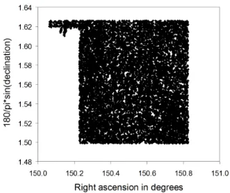
= 4 (180=)0:075 2 = 5500038: (3) The reported survey coverage area of the zCosmos-deep field is 1 deg2, [8]. However, what is required is the solid angle which is measured by the area of the survey projected in the plan described by the right ascension in degrees and
180= sin(declination). Note that the sine of declination term is due to the Jacobian for spherical coordinates. The spectroscopic area obtained with this procedure is 0.075 deg2 (surface coverage in figure 1).
2.1.2 Conversion of redshifts to LTDs
Two approaches are available for converting the redshifts from observed galaxies into LTDs, one based on cosmologi-cal redshifts and the other one on dopplerian redshifts. First, let us introduce the method based on cosmological redshifts from the calculator of Wright [16] which uses a Lambda-CDM cosmology. The followings are generally assumed for this model: a flat Universe, with parameters: M =0.27,
Fig. 1: Procedure to compute the spectroscopic area for the zCosmos survey as defined by the solid angle.
In the dopplerian redshift method, the relationship be-tween redshifts and recession velocities is the following:
1 + z = s
1 +v c
1 v c
: (4)
From this equation, one may compute the recession ve-locity for a given redshift. Then the distance is computed as following:
distance =Hv
o: (5)
From subsequent calculations an M of 0.19 was obtained which was used to derive the galactic density profile. Both methods give comparable distances with differences less than 5%for redshifts up to 5.2 usingM =0.19. The dif-ference between dopplerian and cosmological redshifts is dis-cussed by Bedran [2]. Historically, the first solution to com-pute distances from cosmological redshifts was obtained by Mattig [9] which is based on Friedmann equations of general relativity. Mattig equation withqo =0.5 also provides dis-tances close to what is obtained using dopplerian redshifts; however, Mattig had to assume that conservation of mass is applicable to the Universe in his derivations which is a big bang cosmology. On the other hand, dopplerian redshifts do not require any assumption on the cosmology, and present the advantage that they also explain blueshifts that are being ob-served such as for Andromeda.
2.1.3 Sources of data
The zCosmos galactic survey Data Release DR1 was used [8].
2.2 Propagation of light in an expanding space
The main hypothesis for the development of a model for the propagation of light in an expanding space, is that the speed of light is frame-independent. Considering redshifts, this means that the relative movement of a light source does not change the speed of light emitted; however, it does add or subtract energy to the photon. In a dopplerian world, this change in energy level changes the frequency of the source of light, and not the speed. However, as space between the photon and the observer expands, this expansion is added to the overall dis-tance the photon has to travel in order to reach the observer - in over words the speed of light is frame-independent with respect to the local space. This implies that there exists a distance for which the recession speed between the observer and the photon equals the speed of light, which is the Hubble sphere, and that recession speed can exceed than the speed of light for large distances. The frame-independent hypothesis for the speed of light has been established in the past with the experiment of Michelson-Morley [10]. Based on obser-vations of double stars [14, 4] it was shown that the velocity of propagation of light does not depend on the velocity of motion of the body emitting the light.
As a consequence of the above, LTDs are not anymore ad-ditive, meaning that if we have three points aligned in space, the distance between the two extremes is not anymore equal to the sum of the two sub-segments as measured in LTDs.
Based on the above hypothesis, the Euclidean distance be-tween the photon and the observer is described by the follow-ing differential equation:
dy
dt = c + Ho c T; (6)
where y is the Euclidean distance between the photon and the observer, T the LTD between the observer and the photon, c the celerity of light, andHothe Hubble constant.
2.3 Conversion of light travel distances to Euclidean dis-tances
Let us consider a photon initially situated at a Euclidean dis-tanceyo from the observer and moving at celerity c in the direction of the observer. Let us sayT is the initial LTD between the photon and the observer, and define the Hubble constant function of LTDs.
The differential equation describing the motion of the photon in the LTD framework is described by eq. (6). By taking a reference point in time in the past, andTbbe today time from this reference point, we getT = Tb t. Hence,
dt = dT. Therefore, eq. (6) becomes:
dy
dT = c Ho c T; (7)
By integration from 0 to T, the following relationship re-lating Euclidean distancesyto light travel distancesT is ob-tained:
y = c T c H2o T2: (8) The corresponding horizon computed by setting dTdy = 0 isTh= H1o which is the Hubble sphere.
2.4 The Hubble constant was determined with respect to LTDs
In general the literature refers to the Hubble constant mea-sured with respect to LTDs. A common way to obtain the Hubble constant is based on standard candles with super-novae and cepheids [13, 1] and the Tully-Fisher relation [5]. Both the standard candle and Tully-Fisher method rely on the distance modulus. As shown below the distance modu-lus gives a measure of LTDs and not Euclidean distances.
Let us recall the derivation of the distance modulus. The magnitude as defined by [12] is:
m = 2:5 log F + K; (9) where m is the magnitude, F the brightness or flux and K a constant. The absolute magnitude is defined as the apparent magnitude measured at 10 parsecs from the source.
Planck’s law for the energy of the photon leads to a red-shift correction to the distance modulus
E =h c ; (10) where E is the energy of the photon, h the Planck’s constant, andthe light wavelength.
The ratio of observed to emitted energy flux is derived from eq. (10), leading to
Eobs
Eemit =
emit
obs =
1
1 + z: (11)
From geometrical considerations, the projected surface of the source of light on the receptor diminishes with a relation-ship proportional to the inverse of square distance from the source of light; hence, the following relationship is obtained for the brightness or flux:
Fobs/ Lemitd2 EEobs
emit; (12)
whereLemit is the emitted luminosity anddthe distance to the source of light.
Combining eq. (9), (11) and (12), we obtain:
m = 2:5 log
Lemit
d2 (1 + z)
+ K: (13)
And, because z is close to zero at 10 Parsec:
M = 2:5 log
Lemit
100
+ K; (14)
whereMis the absolute magnitude.
Hence, the distance modulus, eq. (13) minus (14) is:
m M = 5 + 5 log d + 2:5 log(1 + z); (15) with d in parsec andlogmeans the logarithm to base 10.
The expansion of the Universe adds up to the Euclidean distance, and therefore the apparent magnitude of the source of light is fainter than if no expansion was present.
2.5 Evolution of the galactic density assuming no new galaxy formation
Assuming cosmological redshifts we have:
1 + z = aao
1; (16)
whereaoanda1are respectively the present scale factor and the scale factor at z.
From the conservation of mass the density is proportional to the inverse of the cubic scale factor:
/a13: (17)
Therefore, the model for the evolution of the density with respect to the present density is the following:
t= o (1 + z)3; (18)
wheret is the density in the past at redshift z andois the present density.
3 Results
3.1 A flat density profile using Euclidean distances
Galactic density profiles have been derived for the two antag-onistic scenarios respectively assuming that LTDs are addi-tive, and with the propagation of light in an expanding space (figure 2). Note that the galactic density profiles obtained with cosmological redshifts and dopplerian redshifts are very similar. The highest redshift galaxies observed for the survey (z=5.2) are very close to the Hubble sphere (which are at 13.65 Glyr) as calculated from cosmological redshifts with
m=0.19.
Fig. 2: Galactic density profile derived from the equivalent spheri-cal sampling, where Glyr are billion light years from today. LTDs are obtained from redshift conversion with dopplerian redshifts. The blank dots indicate densities based on LTDs. The solid dots indicate densities obtained with Euclidean distances on the basis of dopple-rian redshifts.
3.2 Estimation ofmatter from galactic counts
The average galactic mass estimated from light deflection [15] is 1:7 1011 M. The Universe mean density is ob-tained by multiplying this figure with the average galactic count per cubic Glyr. Using dopplerian redshits the galac-tic count density is4:6 106counts per cubic Glyr, leading to a mean Universe density of1:84 10 30 g=cm3. Using a Hubble constant of 71km=s=Mpcand recent estimates of the gravitational constant of6:67 10 8cm3=g=sec2[11], the critical density is estimated at9:47 10 30g=cm3(from
c=8G3H2). Therefore, the correspondingmequals to 0.19. Note that smaller values of the Hubble constant would lead to a higherm.
3.3 Estimation of the number of galaxies in the visible Universe
Another challenge is to estimate the number of galaxies in the visible Universe. Using the galactic density in the nearby Universe from figure 2 expressed per cubic Glyr LTD, and the volume of the sphere of radius 14 Gly LTD, the num-ber of galaxies in the visible Universe is estimated at 175 billion. Gott et al. [6] estimated a number of galaxies in the visible Universe at about 170 billion based on the Sloan Digital Sky Survey luminosity function data using the Press-Schechter theory. Both figures are consistent with each other; however, the author believes that these figures need to be re-viewed to account only for the Euclidean radius when com-puting the volume of the visible Universe. As the galactic density profile is flat, it is expected that the estimated number
Fig. 3: Galactic density profile derived from the equivalent spherical sampling, where Gly are billion light years from today. LTDs are ob-tained from redshift conversion with cosmological redshifts (omega matter of 0.19).The solid dots indicate densities obtained with Eu-clidean distances on the basis of cosmological redshifts. The blank dots indicate the theoretical evolution of galaxies assuming that the survey is incomplete (with no new galaxy formation).
of galaxies in the visible Universe is internally consistant with the bulk amount of galaxies observed in the survey converted to spherical values, i.e. multiplying the number of galaxies in the survey (10046 galaxies) by the sphere to survey solid angle ratio, which leads to 5.5 billion galaxies (see Table 1).
4 Discussion
A new approach is proposed in the present study to derive the galactic density profile which is based on the conversion of light travel distances to Euclidean distances. The method has been tested by computing the galactic density profiles based on the data from the zCosmos deep field survey.
Table 1: Estimation of the number of galaxies in the visible Universe (radius 14 Glyr) using LTD distances and Euclidean distances.
Radius of the visible Universe
Galactic density Estimated number of galaxies
Using LTDs 14 Glyr 1:52107counts per
cubic Glyr
175 billion Using Euclidean distances
with dopplerian redshifts
6.90 Glyr 4:60106counts per cubic Glyr
6.3 billion Galaxy count of the survey
converted to spherical values
5.5 billion
of order 200 at redshift 5.2. This discrepancy is unrealisti-cally to large. Clearly more detailed work needs to be carried out to investigate this gap.
By applying conservation of mass, as we approach the singularity of the big bang, the Universe would have been so dense that it is difficult to explain how gravity did not pre-vent the early Universe from collapsing. A possibility is that the Hubble constant was much higher in the past leading to a higher critical density - cosmic inflation would still be neces-sary to overcome this issue. From the present study, the galac-tic density appears to be constant over time, which would corroborate the steady state cosmology of [3, 7]. The other condition being that the Hubble constant remains unchanged over time.
Acknowledgments
This work is based on zCOSMOS observations carried out us-ing the Very Large Telescope at the ESO Paranal Observatory under Programme ID: LP175.A-0839.
Submitted on August 24, 2011/Accepted on September 9, 2011
References
1. Altavilla G., Forentino, G., Marconi M., Musella I., Cappellaro E., Barbon R., Benetti S., Pastorello A., Riello M.,Turatto M., Zampieri L. Cepheid calibration of type Ia supernovae and the Hubble constant. Monthly Notices of the Royal Astronomical Society, 1982, v. 349 (4), 1344–1352.
2. Bedran M.L. A comparison between the Doppler and cosmological red-shifts.American Journal of Physics, 2002, v. 70 (4), 406.
3. Bondi H., Gold T. The Steady-State Theory of the Expanding Universe. Monthly Notices of the Royal Astronomical Society, 1948, v. 108 (3), 252.
4. Brecher K. Is the Speed of Light Independent of the Velocity of the Source?Physical Review Letters, 1977, v. 39 (17), 1051–1054. 5. Freedman W.L., Madore B.F., Gibson B.K., Ferrarese L., Kelson D.D.,
Sakai S., Mould J.R., Kennicut Jr. R.C., Ford H.C., Graham J.K., Huchra J.P., Hugues S.M.G., Illingworth G.D., Macri L.M., Stet-son P.B. Final Results from the Hubble Space Telescope Key Project to Measure the Hubble Constant.The Astrophysical Journal, 2001, v. 553 (1), 47–72.
6. Gott R., Juric M., Schlegel D., Hoyle F., Vogeley M., Tegmark M., Bahcall N., Brinkmann J. A Map of the Universe.The Astrophysical Journal, 2005, v. 624 (2), 463–484.
7. Hoyle F., Burbidge G., Narlikar, J.V. A quasi-steady state cosmological model with creation of matter.The Astrophysical Journal, 1993, v. 410, 437–457.
8. Lilly S.J., Le Fevre O., Renzini A., Zamoranti G., Scodeggio M., Con-tini T., Carollo C.M., Hasinger G., Kneib J.-P., Iovino A., Le Brun V., Maier C., Mainieri V., Mignoli M., Silverman J., Tasca L.A.M., Bol-zonella M., Bongiorno A., Bottini D., Capak P., Caputi K., Cimatti A., Cucciati O., Daddi E., Feldmann R., Franzetti P., Garilli B., Guzzo L., Ilbert O., Kampczyk P., Kovac K., Lamareille F., Leauthaud A., Le Borgne J.-F., McCracken H.J., Marinoni C., Pello R., Ricciardelli E., Scarlata C., Vergani D., Sanders D.B., Schinnerer E., Scoville N., Taniguchi Y., Arnouts S., Aussel H., Bardelli S., Brusa M., Cappi A., Ciliegi P., Finoguenov A., Foucaud S., Franceschini R., Halliday C., Impey C., Knobel C., Koekemoer A., Kurk J., Maccagni D., Maddox S., Marano B., Marconi G., Meneux B., Mobasher B., Moreau C., Peacock J.A., Porciani C., Pozzetti L., Scaramella R., Schiminovich D., Shop-bell P., Smail I., Thompson D., Tresse L., Vettolani G., Zanichelli A., Zucca E. zCosmos: A Large VLT/VIMOS Redshift Survey Covering 0 ¡ z ¡ 3 In The Cosmos Field.The Astrophysical Journal Supplement Series, 2007, v. 172, 70–85.
9. Mattig W. ¨Uber den Zusammenhang zwischen Rotverschiebung und scheinbarer Helligkeit.Astronomische Nachrichten, 1958, v. 284, 109.
10. Michelson A.A., Lorentz H.A., Miller D.C., Kennedy R.J., Hedrick E.R., Epstein P.S. Conference on the Michelson-Morley Experiment Held at Mount Wilson.Astrophysical Journal, 1927, v. 68, 341.
11. Mohr P.J., Taylor B.N. CODATA recommended values of the funda-mental physical constants: 2002.Reviews of Modern Physics, 2005, v. 77, 1–107.
12. Pogson N. Magnitudes of Thirty-six of the Minor Planets for the first day of each month of the year 1857.Monthly Notices of the Royal As-tronomical Society, 1857, v. 17, 12–15.
13. Schaefer B.E. The Peak Brightness of Supernovae in the U Band and the Hubble Constant.The Astrophysical Journal, 1995, v. 450, L5–L9.
14. De Sitter W. A proof of the constancy of the velocity of light. Proceed-ings of the Section of Sciences - Koninkijke Academie van Wetenschap-pen te Amsterdam, 1913, v. 15, 1297.
15. Tyson J.A., Valdes F., Jarvis J.F., Mills A.P.Jr. Galaxy mass distribution from gravitational light deflection.The Astrophysical Journal, 1984, v. 281, L59–L62.