Spectral representation of the annual cycle in the climate change signal

(1)

HESSD

8, 1161–1192, 2011

Spectral representation of the

annual cycle in the climate change signal

T. Bosshard et al.

Title Page

Abstract Introduction

Conclusions References

Tables Figures

◭ ◮

Back Close

Full Screen / Esc

Printer-friendly Version

Interactive Discussion

Discussion

P

a

per

|

Dis

cussion

P

a

per

|

Discussion

P

a

per

|

Discussio

n

P

a

per

|

Hydrol. Earth Syst. Sci. Discuss., 8, 1161–1192, 2011 www.hydrol-earth-syst-sci-discuss.net/8/1161/2011/ doi:10.5194/hessd-8-1161-2011

Hydrology and Earth System Sciences Discussions

This discussion paper is/has been under review for the journal Hydrology and Earth System Sciences (HESS). Please refer to the corresponding final paper in HESS if available.

Spectral representation of the annual

cycle in the climate change signal

T. Bosshard1, S. Kotlarski1, T. Ewen1,*, and C. Sch ¨ar1

1

Insitute for Atmospheric and Climate Science, ETH Zurich, Zurich, Switzerland *

now at: Department of Geography, University of Zurich, Zurich, Switzerland

Received: 26 December 2010 – Accepted: 3 January 2011 – Published: 26 January 2011

Correspondence to: T. Bosshard (thomas.bosshard@env.ethz.ch)

(2)

HESSD

8, 1161–1192, 2011

T. Bosshard et al.

Title Page

Tables Figures

◭ ◮

Back Close

Full Screen / Esc

Discussion

P

a

per

|

Dis

cussion

P

a

per

|

Discussion

P

a

per

|

Discussio

n

P

a

per

|

Abstract

The annual cycle of temperature and precipitation changes as projected by climate models is of fundamental interest in climate impact studies. Its estimation, however, is impaired by natural variability. Using a simple form of the delta change method, we show that on regional scales relevant for hydrological impact models, the projected 5

changes in the annual cycle are prone to sampling artefacts. For precipitation at sta-tion locasta-tions, these artefacts may have amplitudes that are comparable to the climate change signal itself. Therefore, the annual cycle of the climate change signal should be filtered when generating climate change scenarios. We test a spectral smoothing method to remove the artificial fluctuations. Comparison against moving monthly av-10

erages shows that sampling artefacts in the climate change signal can successfully be removed by spectral smoothing. The method is tested at Swiss climate stations and applied to regional climate model output of the ENSEMBLES project. The spectral method performs well, except in cases with a strong annual cycle and large relative precipitation changes.

15

1 Introduction

Impacts of climate change on the hydrological cycle are both of high scientific interest as well as of high relevance for society as a whole. The former is due to the intimate coupling of the hydrological cycle and the climate system (Allen and Ingram, 2002; Wentz et al., 2007; Wild et al., 2008) while the latter is based on the manifold inter-20

actions between the anthroposphere and the hydrosphere (Kundzewicz et al., 2007). Hydrological impact studies focussing on runoffoften use statistically post-processed global climate model (GCM) or regional climate model (RCM) data to drive a hydrolog-ical model (Hay et al., 2000; Leung et al., 2004; Wood et al., 2004; Kay et al., 2006; Buytaert et al., 2010). For this purpose, various statistical post-processing methods 25

(3)

HESSD

8, 1161–1192, 2011

T. Bosshard et al.

Title Page

Tables Figures

◭ ◮

Back Close

Full Screen / Esc

Discussion

P

a

per

|

Dis

cussion

P

a

per

|

Discussion

P

a

per

|

Discussio

n

P

a

per

|

these methods are based on statistical relationships that bridge the spatial and tem-poral gaps between observations and modelled data, and attempt to correct for cli-mate model biases. Most of the available methods focus on the hydrometeorological variables temperature and precipitation (abbreviated as T and P, respectively in the remainder of this article) and usually include some representation of the annual cycle. 5

Natural variability, both on interannual as well as intraannual time scales, impairs pa-rameter estimates of the statistical post-processing methods. The range of the natural variability can be assessed using e.g. resampling techniques. Prudhomme and Davies (2009) and Wood et al. (2004), for example, resampled observed time series to esti-mate the range of natural variability of the cliesti-mate change signal. Cross-validation has 10

also been used to test the robustness of the parameter estimates to interannual vari-ability (Terink et al., 2010; Schmidli et al., 2007; Widmann et al., 2003). However, only a few studies focussing on hydrological impacts have looked in detail at the intraannual variability of the parameters. Smoothing by averaging over seasons (see e.g. Schmidli et al., 2007) or months (see e.g. Middelkoop et al., 2001; Kleinn et al., 2005), is a com-15

mon practise. An appropriate representation of the seasonal cycle, however, is not straightforward. On the one hand, the optimal choice of the averaging period is depen-dent on the magnitude of the natural variability, the spatial averaging and the length of the data records. The stronger the natural variability, the smaller the spatial averag-ing area and the shorter the data record is, the wider the averagaverag-ing window has to be 20

chosen in order to reduce the e_ffects of natural variability on the parameter estimates. On the other hand, hydrological impact modellers are interested in an accurate rep-resentation of the annual cycle and therefore prefer as narrow averaging windows as feasible. The optimal solution is thus not trivial to find and is case dependent. Despite its importance, the discussion of how to optimally represent the annual cycle in climate 25

(4)

HESSD

8, 1161–1192, 2011

T. Bosshard et al.

Title Page

Tables Figures

◭ ◮

Back Close

Full Screen / Esc

Discussion

P

a

per

|

Dis

cussion

P

a

per

|

Discussion

P

a

per

|

Discussio

n

P

a

per

|

This paper elaborates on the representation of the annual cycle in the climate change signal within the delta change post-processing methodology. We chose the delta change method because of its simplicity, but the results appear relevant for more so-phisticated methods as well. The delta change method has been used for hydrological impact studies ever since GCM data became available, and it is still used nowadays 5

(Gleick, 1986; Hay et al., 2000; Prudhomme et al., 2002; Lenderink et al., 2007). More sophisticated combinations of the delta change approach and weather generators have also been developed (Kilsby et al., 2007). It is noteworthy that Gleick (1986) already stressed the importance of representing the climate change throughout the annual cy-cle since seasonal changes tend to cancel each other out in the annual average. 10

Here, we test the influence of sampling variability on the annual cycle of the climate change signal by using moving averages (MA) of different window widths. As an alter-native to the MA, we present a spectral approach to estimate the climate change signal. The spectral estimation produces smoother annual cycles of the climate change sig-nals than MAs. Our analysis is carried out at observational station sites in Switzerland. 15

The paper is structured as follows: in Sect. 2, we present the data used for the study. Section 3 introduces the delta change method and the estimation methods for the annual cycle. In Sect. 4, we study the effects of sampling variability on the estimation of the annual cycle using a stochastic rainfall generator. Section 5 presents the estimation of the annual cycle of the climate change signal using a spectral smoothing method 20

and a comparison to estimates using MAs of 31 days window width. Results at Swiss station sites are shown at the end of this section. Section 6 summarises the findings and discusses their relevance for climate impact studies.

2 Data

We used daily near-surfaceT andP data from 10 GCM-RCM model chains provided 25

(5)

HESSD

8, 1161–1192, 2011

T. Bosshard et al.

Title Page

Tables Figures

◭ ◮

Back Close

Full Screen / Esc

Discussion

P

a

per

|

Dis

cussion

P

a

per

|

Discussion

P

a

per

|

Discussio

n

P

a

per

|

scenario, cover the period 1951–2099 and have a horizontal resolution of about 25 km. We had to exclude the HadCM3Q16 driven model chains due to pronounced summer dryings that caused severe overshooting in the spectral smoothing (see Sect. 5.2 for an explanation).

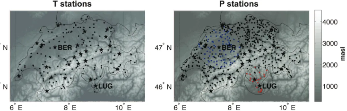
The geographical focus of our study is Switzerland. Throughout this paper, the es-5

timation of the climate change signal is based on RCM data interpolated to station locations of MeteoSwiss (see Fig. 1). All the stations provide T and P data with at least daily resolution in the period 1980–2009. We used the four nearest gridpoints and the inverse distance weighting interpolation algorithm to spatially interpolate the GCM-RCM data to station locations. It should also be noted that any height correction 10

is redundant since constant correction terms cancel each other in the delta change ap-proach. Also, for simplicity, we neglect leap days in the data, unless stated otherwise.

For the stochastic rainfall generator experiments, two subsets of precipitation sta-tions are used to estimate the rainfall generator parameters. These subsets are indi-cated by blue and red dots in Fig. 1 (see also Sect. 4). In addition, we used long-term 15

data series from 26 stations with records going back to 1900 from the climate moni-toring network of MeteoSwiss to constrain the harmonic smoothing model. Stars mark these stations in Fig. 1.

3 Methodology

3.1 The delta change method

20

The delta change method scales station records according to a climate change signal. The climate change signal is usually derived from climate model data as the change between a scenario period (SCE) and a control period (CTL). As a result of the scaling, the spatio-temporal patterns as well as the correlations between the variables closely follow the observed records. Thus, the delta change method is considered a robust 25

(6)

HESSD

8, 1161–1192, 2011

T. Bosshard et al.

Title Page

Tables Figures

◭ ◮

Back Close

Full Screen / Esc

Discussion

P

a

per

|

Dis

cussion

P

a

per

|

Discussion

P

a

per

|

Discussio

n

P

a

per

|

In this study, we applied the delta change method at station sites for the SCE peri-ods 2021–2050 and 2070–2099, both relative to the CTL period 1980–2009. At each stationi, for each RCMjand for each dayd in the year, we estimate the mean annual cycle of the variable of interest and denote it withX_{i ,j}CTL(d) for the control andX_{i ,j}SCE(d) for the scenario period whereX stands for eitherT orP. The delta change method then 5

derives an additive (∆X_{i ,j}add(d)) and a multiplicative (∆X_{i ,j}mult(d)) climate change signal forT andP, respectively, according to

∆T_{i ,j}add(d)=T_{i ,j}SCE(d)−TCTL

i ,j (d) (1)

∆P_{i ,j}mult(d)=

P_{i ,j}SCE(d)

P_{i ,j}CTL(d)

. (2)

LetX_{i ,}CTL_obs(y,d) denote the continuous observational time series at station sites in the 10

CTL period 1980–2009. Here,y represents the years in the CTL period. In the delta change method, all observational time steps in the CTL period belonging to the same dayd in the year are scaled with the corresponding climate change value. Again, one commonly uses an additive or multiplicative scaling forT andP, respectively:

T_{i ,j}SCE,add(y,d)=T_{i ,}CTL_obs(y,d)+ ∆T_{i ,j}add(d) (3) 15

P_{i ,j}SCE,mult(y,d)=P_{i ,}CTL_obs(y,d)·_∆Pmult

i ,j (d) (4)

Equations (1)–(4) reveal that a key issue in the delta change approach is the estimation of the climatological annual cycle in a predefined period. In fact, the delta change ap-proach states nothing but how the climatological annual cycle changes in the transition of the atmospheric state between a CTL and SCE period according to climate model 20

(7)

HESSD

8, 1161–1192, 2011

T. Bosshard et al.

Title Page

Tables Figures

◭ ◮

Back Close

Full Screen / Esc

Discussion

P

a

per

|

Dis

cussion

P

a

per

|

Discussion

P

a

per

|

Discussio

n

P

a

per

|

3.2 Estimation of the climatological annual cycle

It is not possible to derive the true climatological annual cycle of any variable but only an estimate thereof, due to the natural variability and the limited duration of observed or simulated data records. The uncertainty of the estimate might be represented by a stochastic component. Ideally, the estimated climatological annual cycle should be 5

robust and not depend on the stochastic components in the time series while pre-serving the amplitude of the annual cycle. Often, the optimisation of these criteria is a trade-off, and it is not trivial to choose an optimal method to estimate the climatologi-cal annual cycle.

In this study, we used MAs and a spectral approach as an alternative to the MA for 10

the estimation of the climatological annual cycle ofT and P. In the MA approach, the termsX(d)CTL_mod andX(d)SCE_mod in Eqs. (1) and (2) become

X_{i ,j}(d)= 1

ye−ys+1 ye

X

y=y_s

"

1 2n+1

d+n

X

k=d−n

X_{i ,j}(y,k)

#

(5)

whereysandyedenote the start and end year of the chosen period andnstands for the

number of days before and after the dayd in each yeary. We used MAs with window 15

widths of 15 (n=7), 31 (n=15), 61 (n=30) and 91 (n=45) days. The larger then, the smaller the e_ffect of the natural variability on the estimate of the climatological annual cycle. However, the amplitude of the annual cycle is more strongly damped for largern. In the alternative spectral approach, we investigated a spectral reconstruction of the climatological annual cycle by a superposition of harmonics with the base period 20

P=365 d.

Xi ,j(d)=a0_{i ,j}+ H

X

k=1

ak_{i ,j}cos(ωkd)+bk_{i ,j}sin(ωkd)

(6)

ωk= 2kπ

(8)

HESSD

8, 1161–1192, 2011

T. Bosshard et al.

Title Page

Tables Figures

◭ ◮

Back Close

Full Screen / Esc

Discussion

P

a

per

|

Dis

cussion

P

a

per

|

Discussion

P

a

per

|

Discussio

n

P

a

per

|

The superscriptk indicates the order of the harmonic components andH is the max-imum order retained. The coe_fficients ak_{i ,j} and bk_{i ,j} are estimated using the discrete Fourier transform (see e.g. von Storch and Zwiers, 1999) from the daily time series of the RCMj at station sitei in the CTL and SCE period.

For RCMs using the Gregorian calendar, the base periodP is set to 365.25 to ac-5

count for leap years (Narapusetty et al., 2009). The HadCM3Q0 and HadCM3Q3 driven RCMs have a 360 days calendar. For these RCMs, we setP to 360 days. Having esti-mated the harmonically smoothed climatological cycle at each station site and for each RCM, we scale the different lengths of the annual cycle to fit 365 days by choosing P=365 in the reconstruction ofX_{i ,j}(d) as in Eq. (6).

10

In the spectral framework of harmonics, the choice of the maximum order H is the only free parameter. The largerH is, the more the details of the annual cycle can be resolved, but the more vulnerable the spectral model becomes to influences of natural variability and overfitting.

4 Analysis of synthetically generated precipitation time series

15

Let’s assume we could sample two 30 year long precipitation time series from a sta-tionary climate and derive the annual cycle of the precipitation change between the two time series. Stationary here means that the mean climate state is the same in both samples, but the two realisations are modulated by natural variability. Since we know that the climate is stationary by assumption, the asymptotic solution of the precip-20

itation change (expressed as a ration) should equal one representing no precipitation change. Any deviation from one, e.g., the occurence of an annual cycle in the precipi-tation change signal, is solely caused by sampling variability, and does not contain any climate signal.

Here, we investigate the degree of the sampling artefacts in the annual cycle of 25

(9)

HESSD

8, 1161–1192, 2011

T. Bosshard et al.

Title Page

Tables Figures

◭ ◮

Back Close

Full Screen / Esc

Discussion

P

a

per

|

Dis

cussion

P

a

per

|

Discussion

P

a

per

|

Discussio

n

P

a

per

|

precipitation series of individual station sites (STATION) and regions (REGION) both for the northern (CHN) and southern (CHS) parts of Switzerland, in order to study two distinct climates at station and regional scale. Following Wilks and Wilby (1999), we employed a first order Markov chain rainfall generator with the precipitation intensity being modelled by a two-parameter gamma distribution. Letpdwandpwwbe the

transi-5

tion probabilities from a dry to wet and a wet to wet day, respectively. Given realisations of the uniform random number on the unit intervalr₁, the precipitation occurenceY(t) is modelled as

Y(t)= 





1 if Y(t−1)₌0 and r₁≤p_dw

1 if Y(t−1)=1 and r1≤pww

0 otherwise

(8)

where 1 stands for a wet and 0 for a dry day. On wet days, the precipitation intensity 10

I(t) is sampled from a gamma probability density function according to

f(I(t))=(I(t)/β) (α−1)

e(−I(t)/β)

βΓ(α) , I(t),α,β >0 (9)

whereαandβare parameters of the gamma distribution andΓis the gamma function. In this case, the synthetic precipitation time seriesP_synthis derived as

Psynth(t)=Y(t)·I(t) (10)

15

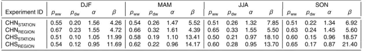
For the single-station experiments CHNSTATION and CHSSTATION, we derived the

pa-rameterspdw,pww,α andβfrom the observed daily precipitation records in the period

1980–2009 at the stations Bern (BER) and Lugano (LUG), respectively. The parame-ters were estimated for each season separately. At the transition from one season to the other, the parameter set is changed but the wet/dry state from the last day of the 20

previous season is taken for the continuation of the Markov chain.

(10)

HESSD

8, 1161–1192, 2011

T. Bosshard et al.

Title Page

Tables Figures

◭ ◮

Back Close

Full Screen / Esc

Discussion

P

a

per

|

Dis

cussion

P

a

per

|

Discussion

P

a

per

|

Discussio

n

P

a

per

|

missing values in the period 1980–2009 and calculated the mean daily precipitation time series therefrom. Remaining missing data were ignored in the averaging. The selected stations are indicated by red and blue dots in Fig. 1. We are aware that this averaging does not follow any spatial interpolation standards. The procedure suffices, though, to analyse the effect of spatial averaging on the fluctuations of the climate 5

change signal. Table 2 lists the seasonal parameter settings for each of the four exper-iments.

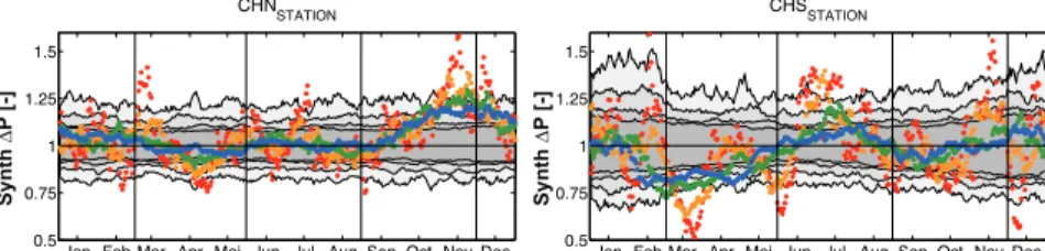
For each experiment, we generated 100 realisations of a daily precipitation time se-ries with a length of 30 years. Subsequently, we randomly chose 500 pairs out of the 100 realisations and calculated the multiplicative precipitation change signal by MAs 10

with window widths of 15, 31, 61 and 91 days. The results are shown in Fig. 2. Since both time series of each pair have been generated with the same rainfall generator settings, the asymptotic solution is one, indicating no change. The dots in Fig. 2 dis-play one randomly chosen realisation of the synthetically generated climate change signal∆Psynth using different MA window widths. The 15d MA estimate shows large

15

fluctuations in every experiment. The wider the MA window becomes, the smaller the fluctuations get. The 31d MA, corresponding to a monthly resolution, is a standard averaging window length in many impact studies. In the 31d MA estimates, the ampli-tudes of the∆Psynth fluctuations are typically in the order of 0.2, but the amplitudes of

spikes can be as large as 0.3 as in the case of CHSSTATION. The grey bands depict the

20

10th–90th% quantile range of the 500 realisations.

Comparison of upper and lower panels in Fig. 2 shows that the spatial averaging does not reduce the band width of the 10th–90th% quantile range substantially. In the CHN experiments, spatial averaging reduces the width of the 31d MA band averaged over the year from 0.87–1.15 to 0.89–1.12 whereas in the CHS cases, the width is 25

reduced from 0.82–1.22 to 0.84–1.19.

(11)

HESSD

8, 1161–1192, 2011

T. Bosshard et al.

Title Page

Tables Figures

◭ ◮

Back Close

Full Screen / Esc

Discussion

P

a

per

|

Dis

cussion

P

a

per

|

Discussion

P

a

per

|

Discussio

n

P

a

per

|

the sampling variability is dependent on the averaging window width, the spatial scale, the region of interest and the length of the climate records. For 31d MAs, our analysis shows for representative climate regions of Switzerland, that∆P values in the range of 0.8 to 1.2 could be solely caused by sampling variability and do not necessarily contain a climate change signal. Furthermore, the spikes within the annual cycles of∆P call 5

for estimation methods that produce smoother climatological annual cycles than MAs.

5 Analysis of the climate change signal from regional climate model at Swiss

station sites

The stochastic analysis in Sect. 4 revealed that for variables having similar character-istics asP, like e.g. a clustering of events and a heavily skewed intensity distribution, 10

estimates of the climate change signal using MAs are prone to substantial artificial fluctuations caused by natural variability. In particular, such fluctuations lead to an impaired representation of the minima and maxima in the annual cycle of the climate change signal. Harmonic smoothing is able to filter these fluctuations. However, the maximal order of the harmonic smoothing model (see Eq. 6) needs to be chosen. In 15

this section we first define the optimal order of the harmonic smoothing model for T andP. We then present a qualitative comparison between the harmonic and the 31 d MA estimates of the climate change signal at station sites, since monthly averaging periods are often employed in climate impact studies. Finally, we show the climate change signals ofT andP estimated by harmonic smoothing for 10 GCM-RCM chains 20

at station sites in Switzerland.

5.1 Estimation of the optimal harmonic model

(12)

HESSD

8, 1161–1192, 2011

T. Bosshard et al.

Title Page

Tables Figures

◭ ◮

Back Close

Full Screen / Esc

Discussion

P

a

per

|

Dis

cussion

P

a

per

|

Discussion

P

a

per

|

Discussio

n

P

a

per

|

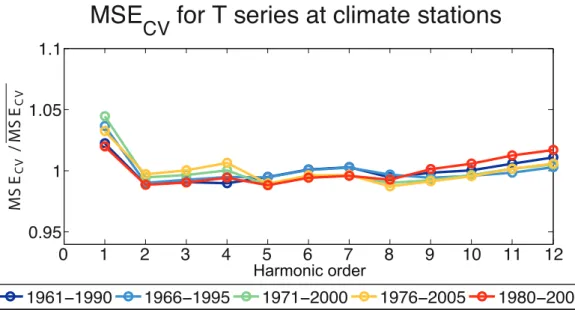
applied to GCM-RCM series. This approach implicitly assumes that signal components from GCM-RCM time series having a higher frequency than the optimal harmonic or-der are consior-dered as being noise. We use a cross-validation technique to specify the harmonic order for the annual cycle that optimally represents the time series. The methodology is described in detail in Narapusetty et al. (2009). Here, we give only 5

a brief introduction and present our specific setup.

We extracted 30 year time slices from 25 temperature and 26 precipitation station records with daily resolution, and split them into ten blocks of three year lengths. Five different 30 year time windows are analysed in order to test the robustness of the results with respect to decadal variability. At each station and for each order of the harmonic 10

smoothing model, we carry out a 10-fold cross-validation by calibrating the harmonic model on 9 of the 10 blocks and validating it on the remaining block. The goal of the cross-validation is to estimate the harmonic model that has the lowest estimated pre-diction error (EPE). The EPE is a measure of the model error in an independent data set that was not used for calibration. It therefore penalises models that are overfitting 15

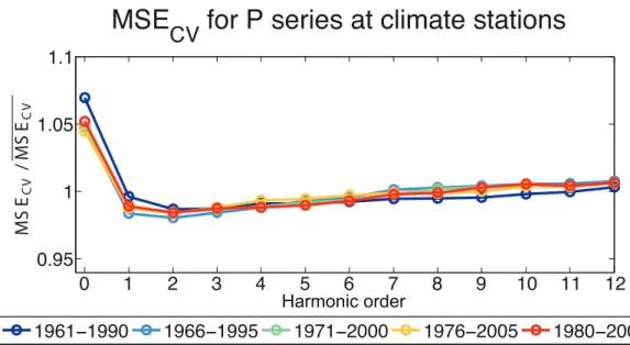
the data. We use the mean squared error (MSE) as a measure for the EPE and call it the cross-validated MSE (MSE_CV). The MSE_CV is optimal for normally distributed and independent residuals. P time series however show strongly non-normal residual distributions. This might cause the estimation of the optimal model to be biased. We therefore first carried out a Box-Cox transformation (Wilks, 2006, p. 43) on theP data. 20

The Box-Cox transformation is a one parametric power-transformation that scales ran-dom variables in a way that their distribution becomes symmetric. Since the Box-Cox transformation only works on positive definite variables, we replaced zeros in the P data by 0.0001.

Figures 3 and 4 show the results of the cross-validation. For T, the MSECV drops

25

to a low level at the harmonic order (HO) of 2 and remains on this low level up to HO 8. Within this plateau, the differences between the models in terms of the MSECV

are small. Depending on the analysis period, the order with the lowest MSECV varies

(13)

HESSD

8, 1161–1192, 2011

T. Bosshard et al.

Title Page

Tables Figures

◭ ◮

Back Close

Full Screen / Esc

Discussion

P

a

per

|

Dis

cussion

P

a

per

|

Discussion

P

a

per

|

Discussio

n

P

a

per

|

orders than HO 8. In the case of P, the MSE_CV has a minimum at HO 2, but the difference to HO 3 is very small. This result is robust for different analysis periods.

The above analysis yields different optimal harmonic orders for T and P. However, as the two atmospheric variables are linked through dynamical and thermodynamical processes, the optimal order for both variables should preferably be the same. We thus 5

chose HO 3 as the optimal order forT andP. With a higher joint HO, we would accept higher-frequency precipitation fluctuations that could stem from natural variability rather than climate change.

5.2 Comparison between the moving average and the spectral estimation of the

climate change signal

10

Based on the results in Sect. 5.1, we use a third order harmonic model (HO 3) to estimate the annual cycle ofP andT in the CTL and SCE periods and compare it to 31d MA estimates. We expect the HO 3 estimates to be characterised by smoother annual cycles and smaller peaks in the annual cycle than 31d MA estimates.

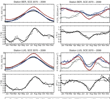
For illustration, Fig. 5 displays annual cycles of P and T at the two station sites 15

BER and LUG as modelled by ETHZ-HadCM3Q0-CLM in the CTL period and the SCE period 2070–2099 as well as the climate change signal (lower panels). These two stations and the selected model chain represent typical results. The annual cycle of the observed values in the CTL period is shown in grey.

In the case ofT, the annual cycle is well captured at both stations, although biases 20

of up to 2 K arise for individual months. The fluctuations in the 31d MA estimate of_∆T have a time scale of typically one month. The amplitudes of these fluctuations are in the order of 0.5–1 K. The HO 3 estimate treats these fluctuations as noise and results in a smooth annual cycle of_∆T.

The depicted precipitation shows a large bias in winter on the northern side of the 25

(14)

HESSD

8, 1161–1192, 2011

T. Bosshard et al.

Title Page

Tables Figures

◭ ◮

Back Close

Full Screen / Esc

Discussion

P

a

per

|

Dis

cussion

P

a

per

|

Discussion

P

a

per

|

Discussio

n

P

a

per

|

the ENSEMBLES RCMs, we refer to Klein Tank et al. (2009) and references therein. The estimates of the climatological annual cycle using a 31d MA show high frequency fluctuations in the CTL and SCE periods, which are amplified in the annual cycle of

∆P due to the division of SCE by CTL values. A spurious amplification can be seen at the station LUG in mid October, when a decrease ofP in the CTL period and a rapid 5

increase in the SCE period occur, leading to a spike in∆P. The HO 3 estimate is not influenced by such high frequency fluctuations and results in a smooth annual cycle.

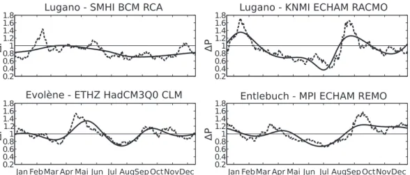
Figure 6 shows further examples of strong fluctuations in the 31d MA around the spectrally smoothed annual cycle ∆P at different station sites and for various model chains. The fluctuations of the 31d MA estimates relative to the spectrally smoothed 10

annual cycles are in the same order of magnitude as the climate change signal. In the spectral smoothing methodology, overshootings can occur in situations when sudden changes in a time series occur within a time scale that cannot be resolved by the spectral model. In our study, serious overshooting problems occured in the case of pronounced summer dryings mainly in Southern Switzerland for model chains driven 15

by the GCM HadCM3Q16. In principle, we could resolve the overshooting problem by a root transformation of the P data. However, such a transformation causes the harmonic smoothing to be non-conservative. We therefore chose not to use a root transformation and exclude the model chains driven by HadCM3Q16 in the current analysis.

20

5.3 Climate change signal at Swiss station sites

5.3.1 Annual cycle of the climate change signal

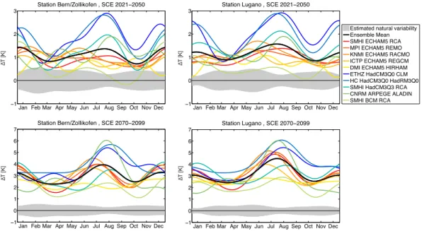
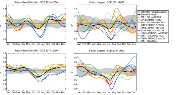
For brevity, we show results of the climate change signal’s annual cycle only at the two exemplary stations BER and LUG (see Fig. 1). Figures 7 and 8 show each RCM’s annual cycle of ∆T and ∆P, respectively for both SCE periods relative to the CTL 25

(15)

HESSD

8, 1161–1192, 2011

T. Bosshard et al.

Title Page

Tables Figures

◭ ◮

Back Close

Full Screen / Esc

Discussion

P

a

per

|

Dis

cussion

P

a

per

|

Discussion

P

a

per

|

Discussio

n

P

a

per

|

100 realisations with a length of 30 years by resampling with replacement the years of the observed record. From the 100 realisations, we randomly chose 500 pairs and estimated the climate change signal between the pairs. The range of±1 standard de-viation (σ) of the 500 resampled realisations is shown as a grey band in Figs. 7 and 8. In the case of_∆T, the ensemble mean shows peaks in winter and summer in both 5

SCE periods. The model spread is largest in summer, which is mainly due to a strong summer warming of HadCM3Q0-driven experiments. Generally, the∆T signal for both SCE periods is distinctively above the estimated natural variability range.

For ∆P, the GCM dominates the climate change signal as can be seen by model chains that use the RCM RCA. The natural variability range of ∆P is much larger 10

relative to the projected_∆P values than in the case of_∆T. Furthermore, the range of natural variability strongly differs from station to station. Only the projected decrease ofP in the summer for the later scenario period is larger than the natural variability for the majority of the RCMs.

5.3.2 Spatial patterns of seasonal mean changes

15

Figures 9 and 10 show the mean seasonal pattern of ∆T and ∆P for both scenario periods. Only the results for the season DJF and JJA are shown since the analysis of the annual cycles showed these seasons to have stronger climate change signals than the transition seasons.

For∆T, the spatial pattern is homogenous across Switzerland with the exception of 20

the Alpine ridge region in JJA that generally shows higher_∆T than other regions in Switzerland. The strongest warming is projected for JJA. The median of all station’s ensemble mean∆T for JJA is 1.4 K for 2021–2050 and 3.7 K for 2070–2099. At most stations, the ensemble mean∆T is larger than 2 times the standard deviation of the natural variability for both scenario periods.

25

(16)

HESSD

8, 1161–1192, 2011

T. Bosshard et al.

Title Page

Tables Figures

◭ ◮

Back Close

Full Screen / Esc

Discussion

P

a

per

|

Dis

cussion

P

a

per

|

Discussion

P

a

per

|

Discussio

n

P

a

per

|

∆P values around 0.7. For DJF, an increase ofP can be expected but the strength of the signal is smaller than for JJA. In the period 2021–2050, the_∆P values generally do not exceed the range of estimated natural variability.

The ensemble mean’s projected seasonal changes for the SCE period 2070–2099 are consistent with the results from the PRUDENCE project (Christensen et al., 2007). 5

In the PRUDENCE project, the ensemble mean∆T in the Alpine region for the SCE period 2070–2100 relative to the CTL period 1961–1990 was+2 K for winter and+4 K for summer. The estimated ensemble mean_∆P was₊10% and −30% for winter and

summer, respectively (Christensen and Christensen, 2007).

6 Summary and conclusions

10

The delta change method commonly used in climate impact modelling studies requires a representation of the climate change signal’s annual cycle. This implies the esti-mation of the annual cycle of T and P both in the CTL and the SCE period. Using a stochastic rainfall generator, we showed that climate change signals of mean precip-itation derived by moving averages are strongly affected by sampling artefacts. Spatial 15

aggregation to a region corresponding to the area of a few RCM grid cells does not reduce the e_ffect of sampling variability on the climate change signal substantially.

Climate change signals estimated using MAs or fixed averaging intervals such as, for e.g., monthly values should thus be regarded with caution, since associated artificial peaks in the annual cycle can lead to undesirable e_ffects when used in combination 20

with non-linear impact models.

We used a spectral smoothing to ameliorate the effects of natural variability on ar-tificial fluctuations in the annual cycle. Compared to 31d MA estimates, the spectral smoothing successfully filters intraannual fluctuations. In a few cases when a strong amplitude of the annual precipitation cycle is paired with a large relative precipitation 25

(17)

HESSD

8, 1161–1192, 2011

T. Bosshard et al.

Title Page

Tables Figures

◭ ◮

Back Close

Full Screen / Esc

Discussion

P

a

per

|

Dis

cussion

P

a

per

|

Discussion

P

a

per

|

Discussio

n

P

a

per

|

The derived climate change signal for the ENSEMBLES GCM-RCM chains is partic-ularly clear for the later SCE period 2070–2099. The peak in the ensembles mean’s

∆T is around 4 K. In the case ofP, a pronounced decrease of summer precipitation is projected for the whole of Switzerland. In the other seasons, precipitation is projected to increase.

5

We focussed on changes in the annual cycle of meanT andP as used in the delta change method. This is a statistical model on the lowest complexity level in the whole variety of statistical post-processing methods. It is a general rule that the more complex models become, for e.g., the more parameters they have, the more prone they are to overfitting. Therefore, it is likely that other post-processing methods such as quantile-10

based de-biasing methods are also a_ffected by artificial fluctuations in the annual cycle of projected changes. Hence, the representation of the annual cycle in any statistical post-processing or downscaling method should be addressed with care.

Acknowledgements. This study was partly funded by swisselectric research, the Federal Office

for the Environment (FOEN) and NCCR climate, a research instrument of the Swiss National

15

Science Foundation. The ENSEMBLES data used in this work was funded by the EU FP6 Integrated Project ENSEMBLES (Contract number 505539) whose support is gratefully ac-knowledged. The observational station data were provided by MeteoSwiss, the Swiss Federal

Office of Meteorology and Climatology. We would also like to thank Lukas Rosinus from the

statistical seminar of the ETH Zurich for his assistance.

20

References

Allen, M. R. and Ingram, W. J.: Constraints on future changes in climate and the hydrologic cycle, Nature, 419, 224–232, 2002. 1162

Buytaert, W., Vuille, M., Dewulf, A., Urrutia, R., Karmalkar, A., and C ´elleri, R.: Uncertainties in climate change projections and regional downscaling in the tropical Andes: implications for

25

(18)

HESSD

8, 1161–1192, 2011

T. Bosshard et al.

Title Page

Tables Figures

◭ ◮

Back Close

Full Screen / Esc

Discussion

P

a

per

|

Dis

cussion

P

a

per

|

Discussion

P

a

per

|

Discussio

n

P

a

per

|

Cameron, D., Beven, K., and Naden, P.: Flood frequency estimation by continuous sim-ulation under climate change (with uncertainty), Hydrol. Earth Syst. Sci., 4, 393–405, doi:10.5194/hess-4-393-2000, 2000. 1163

Christensen, J. H. and Christensen, O. B.: A summary of the PRUDENCE model projections of changes in European climate by the end of this century, Climatic Change, 81, 7–30, 2007.

5

1176

Christensen, J. H., Carter, T. R., Rummukainen, M., and Amanatidis, G.: Evaluating the perfor-mance and utility of regional climate models: the PRUDENCE project, Climatic Change, 81, 1–6, 2007. 1176

Fowler, H. J., Blenkinsop, S., and Tebaldi, C.: Linking climate change modelling to impacts

stud-10

ies: recent advances in downscaling techniques for hydrological modelling, Int. J. Climatol., 27, 1547–1578, 2007. 1162

Gleick, P. H.: Methods for evaluating the regional hydrologic impacts of global climatic changes, J. Hydrol., 88, 97–116, 1986. 1164

Graham, L. P., Hagemann, S., Jaun, S., and Beniston, M.: On interpreting hydrological change

15

from regional climate models, Climatic Change, 81, 97–122, 2007. 1163, 1165

Hay, L. E., Wilby, R. L., and Leavesley, G. H.: A comparison of delta change and downscaled GCM scenarios for three mountainous basins in the United States, J. Am. Water Resour. As., 36, 387–397, 2000. 1162, 1164

Jasper, K., Calanca, P., Gaylistras, D., and Fuhrer, J.: Differential impacts of climate change on

20

the hydrology of two alpine river basins, Clim. Res., 26, 113–129, 2004. 1163

Kay, A. L., Jones, R. G., and Reynard, N. S.: RCM rainfall for UK flood frequency estima-tion, II. Climate change results, J. Hydrol., 318, 163–172, doi:10.1016/j.jhydrol.2005.06.013, 2006. 1162

Kilsby, C. G., Jones, P. D., Burton, A., Ford, A. C., Fowler, H. J., Harpham, C., James, P.,

25

Smith, A., and Wilby, R. L.: A daily weather generator for use in climate change studies, Environ. Modell. Softw., 22, 1705–1719, doi:10.1016/j.envsoft.2007.02.005, 2007. 1164 Klein Tank, A. M. G., Manzini, E., Braconnot, P., Doblas-Reyes, F., Buishand, T. A., and

Morse, A.: Evaluation of the ENSEMBLES Prediction System, chap. 8, Met O_ffice Hadley

Centre, FitzRoy Road, Exeter, EX1 3PB, UK, 2009. 1174

30

(19)

HESSD

8, 1161–1192, 2011

T. Bosshard et al.

Title Page

Tables Figures

◭ ◮

Back Close

Full Screen / Esc

Discussion

P

a

per

|

Dis

cussion

P

a

per

|

Discussion

P

a

per

|

Discussio

n

P

a

per

|

Kundzewicz, Z. W., Mata, L. J., Arnell, N., D ¨oll, P., Kabat, P., Jim ´enez, B., Miller, K., Oki, T., Sen, Z., and Shiklomanov, I.: Freshwater resources and their management, in: Climate Change 2007: Impacts, Adaptation and Vulnerability. Contribution of Working Group II to the Fourth Assessment Report of the Intergovernmental Panel on Climate Change, edited by: Parry, M. L., Canziani, O. F., Palutikof, J. P., van der Linden, P. J., and Hanson, C. E.,

5

Cambridge University Press, Cambridge, UK, 173–210, 2007. 1162

Lenderink, G., Buishand, A., and van Deursen, W.: Estimates of future discharges of the river Rhine using two scenario methodologies: direct versus delta approach, Hydrol. Earth Syst. Sci., 11, 1145–1159, doi:10.5194/hess-11-1145-2007, 2007. 1164

Leung, L. R., Qian, Y., Bian, X., Washington, W. M., Han, J., and Roads, J. O.: Mid-century

10

ensemble regional climate change scenarios for the western United States, Climatic Change, 62, 75–113, 2004. 1162

Middelkoop, H., Daamen, K., Gellens, D., Grabs, W., Kwadijk, J. C. J., Lang, H., Parmet, B. W. A. H., Sch ¨adler, B., Schulla, J., and Wilke, K.: Impact of climate change on hydrological regimes and water resources management in the Rhine basin, Climatic Change, 49, 105–

15

128, 2001. 1163

Narapusetty, B., DelSole, T., and Tippett, M. K.: Optimal Estimation of the Climatological Mean, J. Climate, 22, 4845–4859, doi:10.1175/2009JCLI2944.1, 2009. 1168, 1172

Prudhomme, C. and Davies, H.: Assessing uncertainties in climate change impact analyses on the river flow regimes in the UK, Part 1: baseline climate, Climatic Change, 93, 177–195,

20

doi:10.1007/s10584-008-9464-3, 2009. 1163

Prudhomme, C., Reynard, N., and Crooks, S.: Downscaling of global climate models

for flood frequency analysis: where are we now?, Hydrol. Process., 16, 1137–1150, doi:10.1002/hyp.1054, 2002. 1164

Schmidli, J., Goodess, C. M., Frei, C., Haylock, M. R., Hundecha, Y., Ribalaygua, J.,

25

and Schmith, T.: Statistical and dynamical downscaling of precipitation: an evaluation and comparison of scenarios for the European Alps, J. Geophys. Res., 112, D04105, doi:10.1029/2005JD007026, 2007. 1163

Terink, W., Hurkmans, R. T. W. L., Torfs, P. J. J. F., and Uijlenhoet, R.: Evaluation of a bias cor-rection method applied to downscaled precipitation and temperature reanalysis data for the

30

(20)

HESSD

8, 1161–1192, 2011

T. Bosshard et al.

Title Page

Tables Figures

◭ ◮

Back Close

Full Screen / Esc

Discussion

P

a

per

|

Dis

cussion

P

a

per

|

Discussion

P

a

per

|

Discussio

n

P

a

per

|

van der Linden, P. and Mitchell, J.: ENSEMBLES: Climate Change and its Impacts: Summary

of research and results from the ENSEMBLES Project, Met Office Hadley Centre, FitzRoy

Road, Exeter, EX1 3PB, UK, 2009. 1164

von Storch, H. and Zwiers, F. W.: Statistical Analysis in Climate Research, Cambridge Univer-sity Press, UK, 1999. 1168

5

Wentz, F. J., Ricciardulli, L., Hilburn, K., and Mears, C.: How much more rain will global warming bring, Science, 317, 233, doi:10.1126/science.1140746, 2007. 1162

Widmann, M. L., Bretherton, C. S., and Salath ´e Jr., E. P.: Statistical precipitation downscaling over the northwestern United States using numerically simulated precipitation as a predictor, J. Climate, 16, 799–816, 2003. 1163

10

Wild, M., Grieser, J., and Sch ¨ar, C.: Combined surface solar brightening and increasing green-house effect support recent intensification of the global land-based hydrological cycle, Geo-phys. Res. Lett., 35, L17706, doi:10.1029/2008GL034842, 2008. 1162

Wilks, D. S.: Statistical Methods in the Atmospheric Sciences, vol. 91 of International Geo-physics Series, 2nd edition, Academic Press, 30 Corporate Drive, Suite 400, Burlington,

15

MA 01803, USA, 2006. 1172

Wilks, D. S. and Wilby, R. L.: The weather generation game: a review of stochastic weather models, Prog. Phys. Geog., 23, 329–357, 1999. 1169

Wood, A. W., Leung, L. R., Sridhar, V., and Lettenmaier, D. P.: Hydrologic implications of dy-namical and statistical approaches to downscaling climate model outputs, Climate Change,

20

(21)

HESSD

8, 1161–1192, 2011

T. Bosshard et al.

Title Page

Tables Figures

◭ ◮

Back Close

Full Screen / Esc

Discussion

P

a

per

|

Dis

cussion

P

a

per

|

Discussion

P

a

per

|

Discussio

n

P

a

per

|

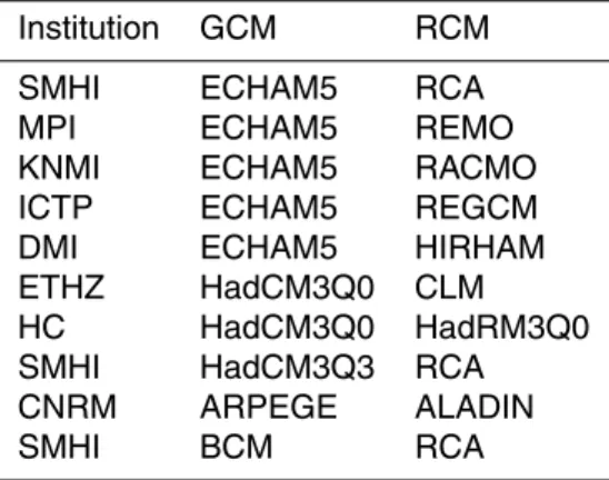
Table 1.List of the employed climate model chains from the ENSEMBLES project.

Institution GCM RCM

SMHI ECHAM5 RCA

MPI ECHAM5 REMO

KNMI ECHAM5 RACMO

ICTP ECHAM5 REGCM

DMI ECHAM5 HIRHAM

ETHZ HadCM3Q0 CLM

HC HadCM3Q0 HadRM3Q0

SMHI HadCM3Q3 RCA

CNRM ARPEGE ALADIN

(22)

HESSD

8, 1161–1192, 2011

T. Bosshard et al.

Title Page

Tables Figures

◭ ◮

Back Close

Full Screen / Esc

Discussion

P

a

per

|

Dis

cussion

P

a

per

|

Discussion

P

a

per

|

Discussio

n

P

a

per

|

Table 2. Seasonal parameter settings of the rainfall generator for the four experiments

CHN_STATION, CHN_REGION, CHS_STATIONand CHS_REGION.

DJF MAM JJA SON

Experiment ID p_ww p_dw α β p_ww p_dw α β p_ww p_dw α β p_ww p_dw α β

CHNSTATION 0.55 0.20 1.56 4.26 0.54 0.26 1.47 5.52 0.51 0.26 1.32 7.85 0.51 0.22 1.34 6.92

CHNREGION 0.67 0.23 1.55 4.72 0.66 0.32 1.61 4.39 0.65 0.33 1.55 5.50 0.63 0.24 1.45 5.60

CHSSTATION 0.51 0.10 1.05 11.99 0.58 0.19 1.10 13.41 0.50 0.21 0.97 18.10 0.60 0.15 0.96 18.57

(23)

HESSD

8, 1161–1192, 2011

T. Bosshard et al.

Title Page

Tables Figures

◭ ◮

Back Close

Full Screen / Esc

Discussion

P

a

per

|

Dis

cussion

P

a

per

|

Discussion

P

a

per

|

Discussio

n

P

a

per

|

Fig. 1. Map with station locations forT (left) andP (right). Stars indicate stations belonging to

the long-term Swiss climate monitoring network. Blue and red dots show the selected stations

for the CHN_REGION (93 stations) and CHS_REGION (23 stations) experiments, respectively (see

(24)

HESSD

8, 1161–1192, 2011

T. Bosshard et al.

Title Page

Tables Figures

◭ ◮

Back Close

Full Screen / Esc

Discussion

P

a

per

|

Dis

cussion

P

a

per

|

Discussion

P

a

per

|

Discussio

n

P

a

per

|

Jan Feb Mar Apr Mai Jun Jul Aug Sep Oct Nov Dec 0.5

0.75 1 1.25 1.5

CHN

STATION

Synth ∆P

[-]

0.75 1 1.25 1.5

D

CHN

REGION

0.75 1 1.25 1.5

CHS_REGION

0.75 1 1.25 1.5

CHS

STATION

MA 15d MA 31d MA 61d MA 91d 10−90% Q. 15d MA 10−90% Q. 31d MA 10−90% Q. 61d MA 10−90% Q. 91d MA

Synth ∆P

[-]

Synth ∆P

[-]

Synth ∆P

[-]

Fig. 2. Annual cycles of the multplicative precipitation change signals (Synth∆P) for the four

experiments CHN_STATION, CHS_STATION, CHN_REGION, CHS_REGIONestimated from time series pairs

(25)

HESSD

8, 1161–1192, 2011

T. Bosshard et al.

Title Page

Tables Figures

◭ ◮

Back Close

Full Screen / Esc

Discussion

P

a

per

|

Dis

cussion

P

a

per

|

Discussion

P

a

per

|

Discussio

n

P

a

per

|

0.95 1 1.05 1.1

0 1 2 3 4 5 6 7 8 9 10 11 12

MS

ECV

/

MS

ECV

MSE

CV

for T series at climate stations

1961−1990 1966−1995 1971−2000 1976−2005 1980−2009

Harmonic order

Fig. 3.Mean over all station’s MSE_CVof harmonic models with increasing harmonic order (HO 1

to HO 12) for observed dailyT series at Swiss climate monitoring stations (see Fig. 1). Results

of five 30 year periods are shown in different colours. The MSE_CV have been normalised by

the mean MSE_CVfor display reasons. The MSE_CVof HO 0 is much larger compared to higher

(26)

HESSD

8, 1161–1192, 2011

T. Bosshard et al.

Title Page

Tables Figures

◭ ◮

Back Close

Full Screen / Esc

Discussion

P

a

per

|

Dis

cussion

P

a

per

|

Discussion

P

a

per

|

Discussio

n

P

a

per

|

0.95 1 1.05 1.1

0 1 2 3 4 5 6 7 8 9 10 11 12

MS

ECV

/

MS

ECV

MSE

CV

for P series at climate stations

1961−1990 1966−1995 1971−2000 1976−2005 1980−2009

Harmonic order

(27)

HESSD

8, 1161–1192, 2011

T. Bosshard et al.

Title Page Abstract Introduction Conclusions References Tables Figures ◭ ◮ ◭ ◮ Back Close

Full Screen / Esc

Printer-friendly Version Interactive Discussion Discussion P a per | Dis cussion P a per | Discussion P a per | Discussio n P a per | 0 10 20 30

Station BER, SCE 2070 − 2099

T CTL, SCE [°C]

Jan Feb Mar Apr May Jun Jul Aug Sep Oct Nov Dec 2.0 2.5 3.0 3.5 4.0 4.5 5.0 5.5 6.0 Δ T [K] Δ 0 5 10

Station LUG, SCE 2070 − 2099

P CTL, SCE [mm d

-1]

Jan Feb Mar Apr May Jun Jul Aug Sep Oct Nov Dec 0.2 0.4 0.6 0.8 1 1.2 1.4 P [−] 0 10 20 30

Station LUG, SCE 2070 − 2099

T CTL, SCE [°C]

Jan Feb Mar Apr May Jun Jul Aug Sep Oct Nov Dec 2.0 2.5 3.0 3.5 4.0 4.5 5.0 5.5 6.0 Δ T [K]

Obs HO3 Obs 31d MA CTL HO3 CTL 31d MA SCE HO3 SCE 31d MA Δ HO3 Δ 31d MA

Δ 0 2 4 6 8

Station BER, SCE 2070 − 2099

P CTL, SCE [mm d

-1]

Jan Feb Mar Apr May Jun Jul Aug Sep Oct Nov Dec 0.2 0.4 0.6 0.8 1 1.2 1.4 P [−] Δ

Fig. 5. Comparison between annual cycles estimated by a 31d MA (dashed lines) and a third

order harmonic smoothing (HO 3; solid lines). Annual cycles ofT andP are displayed in the left

(28)

HESSD

8, 1161–1192, 2011

T. Bosshard et al.

Title Page

Tables Figures

◭ ◮

Back Close

Full Screen / Esc

Discussion

P

a

per

|

Dis

cussion

P

a

per

|

Discussion

P

a

per

|

Discussio

n

P

a

per

|

Fig. 6. Examples of _∆P as estimated by 31d MA (dashed lines) and the spectral smoothing

(29)

HESSD

8, 1161–1192, 2011

T. Bosshard et al.

Title Page

Tables Figures

◭ ◮

Back Close

Full Screen / Esc

Discussion

P

a

per

|

Dis

cussion

P

a

per

|

Discussion

P

a

per

|

Discussio

n

P

a

per

|

∆T [K]

Jan Feb Mar Apr May Jun Jul Aug Sep Oct Nov Dec −1

0 1 2 3

Station Bern/Zollikofen , SCE 2021−2050

0 1 2 3 4 5 6 7

Station Lugano , SCE 2070−2099

∆T [K]

0 1 2 3

Estimated natural variability Ensemble Mean SMHI ECHAM5 RCA MPI ECHAM5 REMO KNMI ECHAM5 RACMO ICTP ECHAM5 REGCM DMI ECHAM5 HIRHAM ETHZ HadCM3Q0 CLM HC HadCM3Q0 HadRM3Q0 SMHI HadCM3Q3 RCA CNRM ARPEGE ALADIN SMHI BCM RCA

Fig. 7. Annual cycle of_∆T for the scenario period 2021–2050 (top) and 2070–2099 (bottom)

(30)

HESSD

8, 1161–1192, 2011

T. Bosshard et al.

Title Page

Tables Figures

◭ ◮

Back Close

Full Screen / Esc

Discussion

P

a

per

|

Dis

cussion

P

a

per

|

Discussion

P

a

per

|

Discussio

n

P

a

per

|

∆P [−]

Jan Feb Mar Apr May Jun Jul Aug Sep Oct Nov Dec 0.6

0.8 1 1.2 1.4

0.4 0.6 0.8 1 1.2 1.4 1.6 1.8

0.8 1 1.2 1.4

Estimated natural variability Ensemble Mean SMHI ECHAM5 RCA MPI ECHAM5 REMO KNMI ECHAM5 RACMO ICTP ECHAM5 REGCM DMI ECHAM5 HIRHAM ETHZ HadCM3Q0 CLM HC HadCM3Q0 HadRM3Q0 SMHI HadCM3Q3 RCA CNRM ARPEGE ALADIN SMHI BCM RCA

0.4 0.6 0.8 1 1.2 1.4 1.6 1.8

∆P [−]

(31)

HESSD

8, 1161–1192, 2011

T. Bosshard et al.

Title Page

Tables Figures

◭ ◮

Back Close

Full Screen / Esc

Discussion

P

a

per

|

Dis

cussion

P

a

per

|

Discussion

P

a

per

|

Discussio

n

P

a

per

|

Ensemble mean,

∆ T, season DJF, 1980−2009 vs. 2021−2050

6°_E ₈°_E ₁₀°_E

46° N 47° N

Ensemble mean,

∆ T, season DJF, 1980−2009 vs. 2070−2099

6° E 8° E 10° E 46° N

47°_N

Ensemble mean,

∆ T, season JJA, 1980−2009 vs. 2070−2099

6° E 8° E 10° E 46° N

47°_N

Ensemble mean,

∆ T, season JJA, 1980−2009 vs. 2021−2050

6°_E ₈°_E ₁₀°_E

46° N 47° N

0 1 2 3 4 5

∆≤ 1 STD 1 STD < ∆≤ 2 STD

∆ > 2 STD

[K]

Fig. 9. Seasonal ensemble mean_∆T at all station sites for both scenario periods 2021–2050

(top) and 2070–2099 (bottom) and the seasons DJF (left) and JJA (right). The colour scale

indicates the ensemble mean value of∆T. The size of the dot indicates the magnitude of∆T

(32)

HESSD

8, 1161–1192, 2011

T. Bosshard et al.

Title Page

Tables Figures

◭ ◮

Back Close

Full Screen / Esc

Discussion

P

a

per

|

Dis

cussion

P

a

per

|

Discussion

P

a

per

|

Discussio

n

P

a

per

|

Ensemble mean,

∆ P, season DJF, 1980−2009 vs. 2021−2050

6° E 8° E 10° E 46° N

47° N

Ensemble mean,

∆ P, season DJF, 1980−2009 vs. 2070−2099

6° E 8° E 10° E 46° N

47° N

Ensemble mean,

∆ P, season JJA, 1980−2009 vs. 2070−2099

6° E 8° E 10° E 46° N

47° N

Ensemble mean,

∆ P, season JJA, 1980−2009 vs. 2021−2050

6° E 8° E 10° E 46° N

47° N

0.7 0.85 1 1.15 1.3

∆≤ 1 STD 1 STD < ∆≤ 2 STD

∆ > 2 STD

[-]