www.the-cryosphere.net/8/1429/2014/ doi:10.5194/tc-8-1429-2014
© Author(s) 2014. CC Attribution 3.0 License.
Representing moisture fluxes and phase changes in glacier debris
cover using a reservoir approach
E. Collier1,4, L. I. Nicholson2, B. W. Brock3, F. Maussion2,4, R. Essery5, and A. B. G. Bush1 1Department of Earth & Atmospheric Sciences, University of Alberta, Edmonton, Canada 2Institute of Meteorology and Geophysics, University of Innsbruck, Innsbruck, Austria 3Geography Department, Northumbria University, Newcastle upon Tyne, UK
4Chair of Climatology, Technische Universität Berlin, Berlin, Germany 5School of Geosciences, University of Edinburgh, Edinburgh, Scotland Correspondence to:E. Collier ([email protected])
Received: 27 February 2014 – Published in The Cryosphere Discuss.: 19 March 2014 Revised: 16 June 2014 – Accepted: 24 June 2014 – Published: 5 August 2014
Abstract. Due to the complexity of treating moisture in supraglacial debris, surface energy balance models to date have neglected moisture infiltration and phase changes in the debris layer. The latent heat flux (QL) is also often excluded due to the uncertainty in determining the surface vapour pres-sure. To quantify the importance of moisture on the surface energy and climatic mass balance (CMB) of debris-covered glaciers, we developed a simple reservoir parameterization for the debris ice and water content, as well as an estima-tion of the latent heat flux. The parameterizaestima-tion was in-corporated into a CMB model adapted for debris-covered glaciers. We present the results of two point simulations, using both our new “moist” and the conventional “dry” ap-proaches, on the Miage Glacier, Italy, during summer 2008 and fall 2011. The former year coincides with available in situ glaciological and meteorological measurements, includ-ing the first eddy-covariance measurements of the turbulent fluxes over supraglacial debris, while the latter contains two refreeze events that permit evaluation of the influence of phase changes. The simulations demonstrate a clear influ-ence of moisture on the glacier energy and mass-balance dy-namics. When water and ice are considered, heat transmis-sion to the underlying glacier ice is lower, as the effective thermal diffusivity of the saturated debris layers is reduced by increases in both the density and the specific heat capac-ity of the layers. In combination with surface heat extraction by QL, subdebris ice melt is reduced by 3.1 % in 2008 and by 7.0 % in 2011 when moisture effects are included. However, the influence of the parameterization on the total
accumu-lated mass balance varies seasonally. In summer 2008, mass loss due to surface vapour fluxes more than compensates for the reduction in ice melt, such that the total ablation increases by 4.0 %. Conversely, in fall 2011, the modulation of basal debris temperature by debris ice results in a decrease in total ablation of 2.1 %. Although the parameterization is a simpli-fied representation of the moist physics of glacier debris, it is a novel attempt at including moisture in a numerical model of debris-covered glaciers and one that opens up additional avenues for future research.
1 Introduction
Numerical modelling of debris-covered glaciers has received renewed scientific interest in recent years, because their con-tribution to changes in ice mass and water resources in many regions remains poorly understood (e.g. Kääb et al., 2012) and because the proportion of debris-covered glacier area is rising as glaciers recede (e.g. Stokes et al., 2007; Bolch et al., 2008; Bhambri et al., 2011).
(e.g. Østrem, 1959; Loomis, 1970; Fujii, 1977; Inoue and Yoshida, 1980; Mattson et al., 1993). The presence of debris also alters the glacier surface energy balance, by permitting surface temperatures to rise above the melting point and by altering surface heat and moisture exchanges with the atmo-sphere (e.g. Brock et al., 2010).
Numerous point models of the surface energy balance of debris-covered glaciers have been developed to simulate sub-debris ice melt (e.g. Kraus, 1975; Nakawo and Young, 1982; Han et al., 2006; Nicholson and Benn, 2006; Reid and Brock, 2010). In recent years, models of debris cover have been ex-tended to distributed simulations (Zhang et al., 2011), and to include both explicit calculation of heat conduction through debris layers resolved into multiple levels and snow accumu-lation on top of the debris (Reid et al., 2012; Lejeune et al., 2013; Fyffe et al., 2014).
However, due to the complexity of treating moisture in supraglacial debris cover, surface energy balance models to date have neglected the latent heat and surface moisture flux components, with the exception of (1) testing the two end-member cases of completely dry or completely saturated de-bris layers (e.g. Nakawo and Young, 1981; Kayastha et al., 2000; Nicholson and Benn, 2006), and (2) using measure-ments of surface relative humidity to calculate the flux when the surface is saturated (Reid and Brock, 2010; Reid et al., 2012). In addition, moisture inputs to the debris layer – by percolation of snowmelt and rainfall, or from the underly-ing meltunderly-ing ice via capillary action – and their phase changes have not been taken into account. Rather, any water is as-sumed to run off immediately, without influencing the ther-mal properties of the debris (e.g. Reid and Brock, 2010; Reid et al., 2012; Lejeune et al., 2013; Fyffe et al., 2014).
Both field observations and laboratory experiments indi-cate that debris covers can be partially or entirely saturated at times during the ablation season, depending on their thick-ness and the environmental conditions, with a minimum of a saturated region adjacent to the interface if the underly-ing ice is at the meltunderly-ing point (e.g. Nakawo and Young, 1981; Conway and Rasmussen, 2000; Kayastha et al., 2000; Reznichenko et al., 2010; Nicholson and Benn, 2012). The presence of interstitial water and ice modifies the thermal properties of the debris layer, particularly during transition seasons (e.g. Conway and Rasmussen, 2000; Nicholson and Benn, 2012). In addition, percolation of rain through a de-bris layer, which can reach as high as 75 % of the total rain-fall at the surface (Sakai et al., 2004), and other inputs of moisture can influence the thermal regime by heat advec-tion (Reznichenko et al., 2010), and by providing a source of moisture for evaporation that cools the debris and there-fore reduces heat transmission to the ice below.
Surface vapour exchanges between the debris and the overlying atmosphere influence the surface energy balance and have been observed to be non-negligible at times. Sakai et al. (2004) estimated that the ablation calculated by an en-ergy balance approach that neglects the latent heat flux, QL,
would provide an overestimate of up to 100 %, since its low-ering effect on surface temperature would not be captured. During the ablation season on the Miage Glacier in the Italian Alps, Brock et al. (2010) calculated large spikes in QL, of up to−800 W m−2, that coincided with daytime rainfall events on the heated debris surface. Furthermore, while they esti-mated that energy inputs due to condensation and deposition were negligible, ground frosts were observed on a weekly to biweekly basis in the upper parts of the glacier, which may have slowed early daytime heating of the debris layer. Given the clear influence of moisture on the surface energy balance and the subsurface thermal regime, there is a need to develop a treatment for moisture fluxes into and within the debris layer, as well as for phase changes, that would allow for a variation in the thermal properties and energy sources and sinks of the debris layer with depth and time.
In this paper, we explore the utility of a reservoir scheme for parameterizing moisture fluxes and phase changes in a glacier debris layer that has been incorporated into a glacier climatic mass balance model. We exploit a short period of available in situ measurements over supraglacial debris to evaluate the model performance during an ablation season, with a second simulation of a fall season to fully demon-strate the capabilities of the model. Within the context of the simplified parameterization, we show the influence of mois-ture on heat transfer in the debris layer, its physical prop-erties, and subdebris ice melt, as well as assess the scale of the impact of phase changes. The eventual goal of this work is to incorporate the debris modifications into an in-teractively coupled modelling system of the atmosphere and alpine glaciers at the regional scale (Collier et al., 2013). The inclusion of debris is essential for (1) accurately capturing surface conditions over debris-covered glaciers and, there-fore, atmosphere–glacier feedbacks, and (2) rigorously as-sessing regional climatic influences on the CMB of debris-covered glaciers.
2 Methods
2.1 Debris-free glacier CMB model
The debris-free version of the glacier CMB model is de-scribed in detail by Mölg et al. (2008, 2009, 2012). The model has been applied to simulating glaciers in a wide variety of climatic settings (e.g. Mölg et al., 2012; Collier et al., 2013; Nicholson et al., 2013; MacDonell et al., 2013). The CMB model solves the surface energy balance equation to determine the energy available for melt and other mass fluxes, given by
S↓ ·(1−α)+ǫ·(L↓ −σ·TSFC4 )+QS+QL
+QG+QPRC=FNET, (1)
Table 1.Physical parameter values used in the CMB models.
Density (kg m−3)
ice 915 –
whole rock 1496 Brock et al. (2010)
water 1000 –
Specific heat capacity (J kg−1K−1)
air 1005 –
ice 2106 –
whole rock 948 Brock et al. (2010)
water 4181 –
Thermal conductivity (W m−1K−1)
air 0.024 –
ice 2.51 –
whole rock 0.94 Reid and Brock (2010)
water 0.58 –
Surface roughness length (m−1)
ice 0.001 Reid and Brock (2010) debris 0.016 Brock et al. (2010)
Albedo
ice 0.34 Brock et al. (2010) firn 0.52 Brock et al. (2010) fresh snow 0.85 Mölg et al. (2012) debris 0.13 Brock et al. (2010)
Emissivity
ice/snow 0.97 Brock et al. (2010) debris 0.94 Brock et al. (2010)
latent heat, the ground heat flux (composed of conduc-tion and penetrating shortwave radiaconduc-tion) and the heat flux from precipitation. Following the convention in mass bal-ance modelling, fluxes are defined as positive when energy transfer is to the surface. The residual energy flux, FNET, constitutes the energy available for melt provided the sur-face temperature has reached the melting point. The specific mass balance is calculated from solid precipitation, surface vapour fluxes, surface and subsurface melt, and refreeze of liquid water in the snowpack. Surface vapour fluxes (Mv; i.e. sublimation or deposition (kg m−2) depending on the sign of QL) at each time step1tare calculated according to
Mv= QL·1t
LH
, (2)
whereLHis the latent heat of sublimation (2.84×10⁶J kg−1) or vaporization (2.51×10⁶J kg−1), depending on the sur-face temperature. The CMB model treats numerous addi-tional processes, including the evolution of surface albedo and roughness based on snow depth and age; snowpack com-paction and densification by refreeze; and the influence of penetrating solar radiation, refreeze and conduction on the near-surface englacial temperature distribution. Physical pa-rameter values for snow and ice are provided in Table 1.
2.2 Inclusion of debris
For this study, the glacier CMB model was modified to in-clude a treatment for supraglacial debris according to two cases: (1) one with no treatment of moisture fluxes or phase changes in the debris layer, congruent with previous studies (CMB-DRY); and (2) one that introduces a reservoir to pa-rameterize the moisture content of the debris layer and its phase, and also includes a latent heat flux calculation (CMB-RES). The simulations are performed as point simulations, due to the availability of both meteorological-forcing and evaluation data at a single location.
2.2.1 Surface temperature
Consistent with previous modelling studies of debris-covered glaciers (e.g. Nicholson and Benn, 2006; Reid and Brock, 2010; Reid et al., 2012; Zhang et al., 2011), the model em-ploys an iterative approach to prognosing surface tempera-ture, with the solution yielding zero residual flux in the sur-face energy balance (Eq. 1). The model uses the Newton– Raphson method to calculateTSFCat each time step, as im-plemented in Reid and Brock (2010), with a different termi-nation criteria of|FNET|<1×10⁻³. When snow or ice are exposed at the surface, the resultingTSFCis reset to the melt-ing point if it exceeds this value, and energy balance closure is achieved by using the residual energy for surface melt. 2.2.2 Subsurface temperature
Both versions of the CMB model prognose the temperature distribution in the upper subsurface following the conserva-tion of energy. The vertical levels selected for the case study in Sect. 2.3 are defined in Table 2, and are set at fixed depths in the subsurface, from 0.0 to 9.0 m, that track the glacier surface as it moves due to mass loss or gain. On this grid, the 1-D heat equation becomes
ρcdT dt =ρc
∂T ∂t =
∂ ∂z
k∂T ∂z
+∂Q
∂z, (3)
whereρis the density (kg m−3);cis the specific heat capac-ity (J kg−1K−1);T is the englacial temperature (K);kis the thermal conductivity (W m−1K−1); and Qis the heat flux due to non-conductive processes (penetrating shortwave ra-diation; W m−2).
Table 2.Subsurface layer distribution and debris thickness used in this study.
Layers
Every 0.01 m from 0 to .24 m, 0.3, 0.4, 0.5, 0.8, 1.0, 1.4, 2.0, 3.0, 5.0, 7.0, 9.0 m
Debris thickness 0.23 m
approximately linear. The convergence of the numerical so-lution down to a vertical grid spacing of 1 mm was checked; however, the results did not strongly differ from the 1 cm case.
With the exception of Lejeune et al. (2013), the ice tem-perature in previous modelling studies has been assumed to be at the melting point, due to the focus on the ablation sea-son (e.g. Nicholsea-son and Benn, 2006; Reid and Brock, 2010). Although this assumption has been validated by field mea-surements (e.g. Conway and Rasmussen, 2000; Brock et al., 2010), it limits the temporal applicability of the model and may contribute to the overestimation of night-time surface temperatures when the overlying air temperature drops be-low the melting point (Reid and Brock, 2010). The CMB models explicitly simulate heat conduction throughout the glacier column. Therefore, the ice temperature is a prognos-tic variable at all levels except the bottom boundary, where a zero-flux condition is imposed. Finally, subsurface heat-ing due to penetratheat-ing shortwave radiation is not considered when glacier debris is exposed at the surface (e.g. Reid and Brock, 2010).
2.2.3 Physical and thermal properties
The important physical properties of the glacier subsurface in Eq. (3) – densityρ, thermal conductivityk, and specific heat capacity c– are non-uniform with depth. DefiningmS and mD as the levels corresponding to the bottom of the snow-pack and debris layers (cf. Fig. 1), respectively, the column properties (generalized asf (z)) are specified as
f (z)=
fsnow z <=ms fdeb ms< z <=md.
fice z > md
(4)
Standard values are selected for snow and glacial ice proper-ties (Table 1), with the exception of snow density, which is a prognostic variable. Within the debris layer, the properties of each 1 cm layer are a weighted average of the depth-invariant whole-rock values,fwr, and the content of the pore space,fφ,
as determined by an assumed linear porosity function,φ: fdeb(z)=φ (z)·fφ(z)+(1−φ (z))·fwr. (5)
ICE SNOW PRECIPITATION LONGW A VE LONGW A VE QS QL QG QG AIR INFIL TRA TION SUBSFC MELT RUNOFF z=variable z=variable
z= 1 cm
S F C V APOR FLUXES MEL T REFREEZE SHOR TW A VE SHOR TW A VE DEBRIS WATER/ICE mK mS mD
Figure 1.Schematic of the CMB-RES model and its treatment of
the debris moisture content and its phase. The levelsmS,mD, and
mKcorrespond to the bottom of the snowpack, the base of the debris
layer, and the level of the saturated horizon, respectively.
For CMB-DRY, the debris pore space contains only air (fφ=
fair), while the weighted average in CMB-RES also consid-ers the bulk water and ice content of the debris of saturated layers. The porosity function is discussed further in Sect. 2.3. 2.2.4 Moisture in the debris layer
For CMB-DRY, rainfall or other liquid water inputs are in-stantaneously removed as runoff from the debris layer and do not accumulate or contribute to vapour exchanges between the debris and the atmosphere, similar to previous modelling studies (e.g. Reid and Brock, 2010; Reid et al., 2012; Lejeune et al., 2013).
For CMB-RES, a reservoir is introduced for moisture ac-cumulation and phase changes (Fig. 1). The reservoir depth for each column is calculated as the sum of the debris poros-ity over the debris thickness. Thus, the pore space in the de-bris is represented as a single reservoir, rather than the stor-age in each 1 cm layer being treated individually. Liquid wa-ter, from rainfall or melt of the overlying snowpack, instantly infiltrates the reservoir. The location of the water and/or ice in the debris is not prognosed; rather, moisture is assumed to occupy the lowest debris layers, adjacent to the glacier ice.
representation of the runoff timescale, which is a linear func-tion of terrain slope and varies from 1 to 0 h−1between 0◦
and 90◦(Reijmer and Hock, 2008).
Congruent with the simple nature of the reservoir param-eterization, the heat flux from precipitation is only applied at the surface in CMB-RES, and subsurface heat transport by water percolation is not included. This treatment is consistent with the findings of Sakai et al. (2004), namely that the heat flux due to rainfall percolation contributes minimally to sub-debris ice melt, although its influence may depend on sub-debris permeability (Reznichenko et al., 2010).
2.2.5 Turbulent fluxes of latent and sensible heat The turbulent fluxes of sensible heat (both models) and latent heat (CMB-RES) were computed using bulk aerodynamic formulae and corrected for atmospheric stability according to the bulk Richardson number, as is standard in glacier energy balance modelling (e.g. Braithwaite, 1995; Reid and Brock, 2010). The bulk Richardson number was constrained within reasonable limits following Fyffe et al. (2014), with the cor-rection applied to fewer than 2.0 % of total time steps in the simulations. The latent heat flux in CMB-DRY was set to zero, to be consistent with previous studies of debris-covered glaciers, as no measurements of surface relative humidity were available. For CMB-RES, the surface vapour pressure was needed but unknown.
For the case study described in Sect. 2.3, an auto-matic weather station (AWS) measured relative humidity at a height ofzair= 2.16 m, from which the partial vapour pres-sure was calculated. The partial density of water vapour was then obtained from
eair=ρairvapRvTair, (6)
where the symbols correspond to, from left to right, the air’s water vapour partial pressure, the partial density of water vapour, the specific gas constant for water vapour (461.5 J kg−1K−1), and the air temperature at a height of zair. In this study, we assumed thatρairvapis constant between the sensor and the surface of the debris layer, i.e. that water vapour in the atmospheric surface layer is well mixed. The vapour pressure at the surface is therefore given by
e∗sfc=eairTsfc
Tair . (7)
For a completely unsaturated glacier debris layer in CMB-RES, a latent heat flux would nonetheless arise due to the vapour pressure gradient that results from the temperature difference between the surface andzair. However, when wa-ter or ice are present in the debris, the final calculation of the surface vapour pressure,esfc, includes a linear correction towards the saturation valueesfc satatTsfcaccording to
esfc=e∗sfc+ esfc sat−e∗sfc
·
1− 2air φbulk
, (8)
wheree∗
sfcis the initial guess in Eq. (7);2airis the void frac-tion of the bulk layer that is occupied by air; andφbulkis the bulk debris porosity, which is invariant under different debris thicknesses due to the linear specification ofφ(as described in Sect. 2.3).2airis given by
2air=
mK
X
i=1 φi
N, (9)
wheremK is the level of the saturated horizon in the debris andN is the total number of layers in the debris. When the debris is completely unsaturated,2air=φbulk, and when it is completely saturated,2air= 0.
Therefore, the surface vapour pressure in CMB-RES is a linear function of the moisture content of the reservoir rather than a wetted debris surface: as the reservoir fills from infiltration of rainfall or snowmelt, the distance between the surface and the saturated horizon (represented by2air) de-creases andesfcapproaches saturation.
2.2.6 Mass balance
The total mass balance calculation in DRY and CMB-RES accounts for the following mass fluxes (kg m−2) at each time step: solid precipitation, surface and vertically inte-grated subsurface melt, meltwater refreeze and formation of superimposed ice in the snowpack, changes in liquid water storage in the snowpack, and surface vapour fluxes. The con-tribution of surface vapour fluxes to or from the debris layer is zero when overlying snow cover is present and in CMB-DRY. In CMB-RES, these fluxes also contribute to changes in the debris water and ice content of the reservoir. For both models, subdebris ice melt is calculated as the vertical inte-gral of melt in the ice column underlying the debris.
Liquid precipitation contributes indirectly to the mass bal-ance in both CMB models through changes in storage in the snowpack, and contributes directly in CMB-RES, via reser-voir storage. However, changes in the debris water and ice content in CMB-RES are not included in the mass balance calculation, so as to allow for a more direct comparison be-tween CMB-RES and CMB-DRY of the influence of includ-ing the latent heat flux. The impact of changes in the storage of water and ice in the debris is quantified in Sect. 3 and has a negligible influence on the total accumulated mass balance. 2.3 Miage Glacier case study
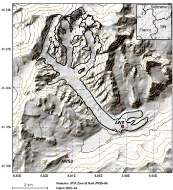
The study area is the Miage Glacier in the Italian Alps (45◦47′N, 6◦52′E; Fig. 2). This glacier was selected due
2000
2000
2000
3000
3000
3000
3000
4000
4000
6.80E 6.82E 6.84E 6.86E 6.88E 6.90E
45.76N 45.78N 45.80N 45.82N 45.84N
6E 7E 8E
45N 46N
France Italy
Switzerland
2 km Projection: UTM, Zone 32 North (WGS−84)Projection: UTM, Zone 32 North (WGS−84) Datum: WGS−84
Datum: WGS−84
AWS2
AWS
Figure 2.Map showing the location of the Miage Glacier. The AWS
located on the glacier is denoted with a red circle and the AWS2 from which precipitation data were obtained is shown by a red tri-angle.
The AWS site was deliberately chosen to be upwind from any nearby large boulders.
We performed two simulations, one for summer 2008 and one for fall 2011. The former covered the period of 25 June– 11 August 2008, with the first 25 days discarded as model spin-up time. For much of the 2008 simulation, the AWS pro-vided hourly values of air temperature, vapour pressure, wind speed, and incoming short- and longwave radiation (Fig. 3). However, during the spin-up period, wind speed and incom-ing longwave radiation were missincom-ing due to a programmincom-ing error in the AWS. To provide this missing data, wind speed was generated synthetically using the hourly average from the measured data during the evaluation period. Incoming longwave radiation was obtained from the ERA-Interim re-analysis (0.75◦×0.75◦ resolution; Dee et al., 2011), using
data from the closest model grid cell after interpolation from 12-hourly to hourly reference points. For the time period where both ERA-Interim and AWS data overlap (20 July– 11 August 2008), the mean deviation (MD) and mean ab-solute deviation (MAD; ERA minus AWS) are ∼13 and ∼35 W m−2, with the deviation likely arising due to the dif-ference between modelled and real terrain height of−450 m. Lastly, a rain gauge was not installed at the AWS site in 2008. We therefore used input data from another AWS located 4 km away (denoted as AWS2 in Fig. 2) and assumed that they were representative of conditions at the AWS on the Miage Glacier.
Table 3.Mean deviation (MD), mean absolute deviation (MAD),
and R value for the evaluation variables of surface temperature (Tsfc), and the turbulent fluxes of sensible (QS) and latent heat (QL).
2008 CMB-DRY CMB-RES
Tsfc MD −0.5 −1.1
MAD 2.3 2.4
R 0.94 0.94
QS MD −65.2 −47.0 MAD 71.1 54.2
R 0.91 0.92
QL MD 23.9 1.0 MAD 28.2 19.1
R – 0.52
2011 CMB-DRY CMB-RES
Tsfc MD 1.1 0.9
MAD 1.9 1.7
R 0.97 0.97
The 2008 simulation was intended to coincide with a sup-plementary field measurement program. Between 20 July and 11 August, surface temperature and the turbulent fluxes of latent and sensible heat were measured. The first field was measured with a CNR1 radiation sensor (Kipp & Zo-nen, Delft, the Netherlands), while the latter two fluxes were measured by an eddy covariance (EC) station. This com-prised a CSAT three-dimensional sonic anemometer and KH2O Krypton Hygrometer (both Campbell Scientific Lim-ited, Shepshed, UK), installed at a height of 2 m above the debris surface. These sensors measured the three compo-nents of turbulent wind velocity, virtual temperature and wa-ter vapour concentrations at an inwa-terval of 50 ms. Raw data were processed using Campbell Scientific OPEC software, which included a “WPL” (Webb–Pearman–Leuning) correc-tion for density effects (Webb et al., 1980) and 30 min aver-ages of the 50 ms scans were stored. The data were filtered for outliers using three times their standard deviation before being used for evaluation (Brock et al., 2010). Surface tem-perature was calculated from the upwelling longwave radia-tion recorded by the CNR1, using an emissivity of 0.94. The AWS tripod provided a stable platform on the slowly melt-ing glacier surface, although the possibility of tiltmelt-ing of the instrument mast cannot be excluded. These measurements provide a unique data set with which to evaluate the CMB models using direct measurement of turbulence in the sur-face atmospheric layer above a debris-covered glacier.
AWS AWS2 ERA Interim (temporally downscaled)
a
b
c
d
e
f
date [2008]
precipitation [mm]
Figure 3.Times series from the 2008 simulation of the forcing variables of(a)2 m air temperature (K),(b)wind speed (m s−1),(c)2 m
vapour pressure (hPa),(d)incoming shortwave radiation (W m−2),(e)incoming longwave radiation (W m−2),(f)surface pressure (hPa), and(g)precipitation (mm). Data from the AWS on the Miage Glacier are shown in black, from the second AWS (4 km away) in blue, and temporally downscaled from the ERA-Interim reanalysis in green. Dashed curves indicate the discarded spin-up period, while solid curves indicate the simulation time.
freezing events, from 18 to 19 September and 7 to 9 Oc-tober 2011. Incoming longwave radiation, precipitation and mean wind speed were available hourly from the AWS (forc-ing data not shown), and measured surface temperature data, estimated from the upwelling longwave radiation recorded by the CNR1, were available for model evaluation.
A final forcing variable for the calculation of the debris surface energy balance, surface pressure, was missing for both the 2008 and 2011 simulations. These data were ob-tained from the ERA-Interim reanalysis, at 6-hourly tempo-ral resolution, and again from the closest grid cell. A correc-tion was applied for the difference between the real and mod-elled terrain height using the hypsometric equation, assum-ing a linear temperature gradient calculated from the AWS and the air temperature on the first model level in the ERA-Interim. For both simulations, the same subsurface layer
spacing was used and is provided in Table 2. The englacial temperature profile was initialized at the melting point, since both simulations began in June. Uncertainties in the temper-ature initialization were addressed by the inclusion of long spin-up periods.
bound of 60 % showed that while subdebris ice melt was strongly affected (it decreased by ∼17 % in both simula-tions), the CMB model behaviour and the main results pre-sented in Sect. 3 remained intact. Other physical and thermal properties of the column were either taken from field mea-surements or specified from values used in previous mod-elling studies of this glacier (e.g. Reid and Brock, 2010). The porosity value of 20 % in the lowest 1 cm layer in the debris gave a minimum water content of 2 kg m−2that was imposed only when the subdebris ice was at the melting point. Subde-bris ice melt changes by ±1.8 % if the minimum value is removed or doubled in the 2008 simulation.
A slope of 7◦ at the AWS gives a runoff timescale of
0.92 h−1. This simple representation of runoff timescales does not consider contributions from upslope regions in the glacier; however, we feel that this is an appropriate first step given that horizontal transport of water within the debris is poorly constrained and no measurements are available. Vary-ing the runoff timescale by±4 % (equivalent to changing the slope from 4◦ to 10◦) results in small changes in total
ac-cumulated mass balance and subdebris ice melt during the summer 2008 simulation, of less than±0.6 and±0.4 %, re-spectively. The results in the transition season of fall 2011 are more sensitive, with changes in these variables of up to ±1.0 and±2.0 %, respectively.
Finally, although the CMB models are evaluated against a short summer period in 2008 and in fall 2011, they are ap-plicable throughout the annual cycle and to glaciers of any temperature regime, as illustrated in Fig. 1.
3 Results
3.1 Comparison with in situ measurements
The surface temperatures (Tsfc) simulated by CMB-DRY and CMB-RES are in good agreement with measurements for both the 2008 and 2011 simulations (Fig. 4a, d; Table 3). The models tend to underestimate daily maximum tempera-tures in 2008 and night-time radiative cooling in 2011. How-ever, for both simulations, the models reproduce the diurnal cycle and its variability well. The CMB models also cap-ture the variability of the sensible heat flux (QS), but the simulated magnitude of heat transfer to the overlying atmo-sphere is greater than reported by the EC station (Fig. 4b). The overestimation of QS for the CMB-DRY run is in part attributable to the lack of latent heat flux (QL), which means that an average energy loss of ∼24 W m−2 is not captured (Fig. 4c; cf. Table 3). CMB-RES has a greatly reduced but still non-negligible bias in QS, again, in part, because evapo-rative cooling is underestimated, by∼6 W m−2. The smaller simulated latent heat flux compared with the EC data re-sults from the approach used to estimate surface vapour pres-sure (cf. Sect. 2.2), which produces an average gradient of
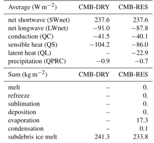
Table 4.Average-energy and accumulated-mass fluxes at the
sur-face over the 2008 simulation for CMB-RES and CMB-DRY.
Average (W m−2) CMB-DRY CMB-RES
net shortwave (SWnet) 237.6 237.6 net longwave (LWnet) −91.0 −87.8 conduction (QC) −41.5 −40.1 sensible heat (QS) −104.2 −86.0 latent heat (QL) – −22.9 precipitation (QPRC) −0.9 −0.7 Sum (kg m−2) CMB-DRY CMB-RES
melt – 0.
refreeze – 0.
sublimation – 0.
deposition – 0.
evaporation – 17.3 condensation – 0.1 subdebris ice melt 241.3 233.8
only −0.5 hPa m−1 between the surface and overlying air (Fig. 5a).
3.2 Modelling insights from the 2008 simulation In total, the influence of the reservoir parameterization on the accumulated mass balance between 20 July and 11 Au-gust 2008 is small, increasing from−241.0 kg m−2in CMB-DRY to−250.6 kg m−2 in CMB-RES (Fig. 5b). These val-ues are equivalent to an ablation rate of approximately 11 mm w.e.d−1(w.e. water equivalent), which is in order of magnitude agreement with the value of 22 mm w.e.d−1 re-ported by Fyffe et al. (2012) for the Miage Glacier, based on the entire ablation seasons of 2010 and 2011.
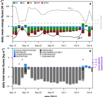
The mass fluxes underlying the simulated mass balance signal are determined by the surface energy balance, whose daily-mean components are shown in Fig. 6a for CMB-RES. Energy receipt, mainly through net shortwave radiation, is generally counteracted by energy losses though net longwave radiation, heat conduction (QC), and the turbulent fluxes QL and QS. The heat flux to the debris surface from precipita-tion (QPRC) has an average value of−12.5 W m−2 during rainfall events. However, since the precipitation temperature is assumed to be the same asTair, QPRC is a stronger energy sink for daytime rainfall. These energy fluxes produce abla-tion that is dominated by subdebris ice melt and evaporaabla-tion over the evaluation period (Fig. 6b; Table 4). Surface melt, refreeze, sublimation and deposition are zero, since there is no solid precipitation and both the debris surface and internal temperatures remain above the melting point.
a
b
c
d
AWS CMB-DRY CMB-RES
Figure 4.Time series from the 2008 simulation of(a)debris surface temperature (Tsfc; K) and the turbulent fluxes of(b)sensible and(c)
latent heat (W m−2), for measurements (black curve), CMB-DRY (dark grey curve), and CMB-RES (blue, dashed curve).(d)Same as panel
a, but for the 2011 simulation. The horizontal dashed red line indicates the freezing point, 273.15 K.
Figure 5. Time series from the 2008 simulation of (a) surface
(dashed-blue curve) and 2 m air (black curve) vapour pressure (hPa) in CMB-RES, and(b)total accumulated mass balance (kg m−2) for CMB-DRY (solid-grey curve) and CMB-RES (dashed-blue curve).
a small reduction in subdebris ice melt, of 7.5 kg m−2 (Ta-ble 4). However, the reduction in melt is more than compen-sated by surface vapour fluxes, with a total of 17.3 kg m−2 of evaporation over the evaluation period. Evaporation
dom-inates during the day (95 % of the total), while smaller amounts of condensation occur mainly at night (64 %) or in the early morning.
SOLID PRECIPITATION REFREEZE CONDENSTATION DEPOSITION
SNOW MELT SUB-DEBRIS ICE MELT EVAPORATION SUBLIMATION
SWNET
LWNET
date [2008]
a
b
mean albedo
accumulated
rainfall [mm]
Figure 6.CMB-RES values for(a)daily mean energy fluxes over
the evaluation period (W m−2). The grey curve is net shortwave radiation, the black curve is net longwave radiation, and the grey dots show daily-mean surface albedo, which remains constant at the debris value because there is no solid precipitation.(b)Daily total mass fluxes (kg m−2). Maximum daily values of evaporation and condensation are 1.4 and 0.02 kg m−2, respectively, although
the latter flux is not visible. Note that while daily-accumulated rain-fall is shown (purple asterisks), it is not technically a mass flux, since the mass balance calculation in CMB-RES does not account for debris-water storage. Rather, this field is plotted to show its cor-respondence with other fields, such as net shortwave radiation.
the “wet” sample time slice) and a smaller effect on the partially saturated layer (at a depth of 19 cm). The debris-specific heat capacity is the most strongly affected physical property, since the value of water is approximately four times that of air (4181 vs. 1005 J kg−1K−1).
The effective thermal diffusivity of the debris is inversely proportional to the specific heat capacity and the debris den-sity. Increases in both these quantities, but particularly in the former, reduce heat diffusion over affected layers compared with CMB-DRY. Therefore, in combination with heat extrac-tion by QL, the change in subsurface physical properties re-duces the amplitude and depth penetration of the diurnal tem-perature cycle in the debris layer (Fig. 9). Fluctuations in the magnitude of QL have a correlation coefficient of 0.78 with the temperature difference between RES and CMB-DRY in the top 6 cm of the debris, while reductions in the effective thermal diffusivity have a correlation coefficient of 0.6 with the temperature difference in the bottom 6 cm.
Table 5.Average-energy and accumulated-mass fluxes at the
sur-face over the 2011 simulation for CMB-RES and CMB-DRY.
Average (W m−2) CMB-DRY CMB-RES
net shortwave (SWnet) 133.0 133.0 net longwave (LWnet) −80.2 −78.8 conduction (QC) −23.0 −22.4 sensible heat (QS) −27.0 −20.0 latent heat (QL) – −9.8 precipitation (QPRC) −0.1 −0.1 Sum (kg m−2) CMB-DRY CMB-RES
melt 4.6 4.4
refreeze 0 0
sublimation 0.2 0.5
deposition 0 0
evaporation – 8.6 condensation – 0.1 subdebris ice melt 172.4 160.4
Figure 7.Time series of total debris-water content (black curve)
as well as the two sources of debris-water loss: horizontal drainage (solid-grey curve) and evaporation (dashed-grey curve). Units are in kilograms per square metre (kg m−2).
3.3 Impact of phase changes in the 2011 simulation Two freezing events occur during the 2011 simulation, be-tween 18 September 23:00 LT (local time) and 19 Septem-ber 14:00 LT and between 7 OctoSeptem-ber 09:00 LT and 9 OctoSeptem-ber 09:00 LT, at the end of two precipitation events with subzero air temperatures (cf. Fig. 4d). Energy and mass fluxes for this simulation are summarized in Table 5.
a
b
c
d
e
f
Figure 8.Depth variation of(a)debris thermal conductivity (W m−1K−1),(b)density (kg m−3), and(c)specific heat capacity (J kg−1K−1),
shown for CMB-DRY in grey-unfilled circles and for CMB-RES in both black-filled circles (“dry” time slice) and blue asterisks (“wet” time slice). Time series of bulk values for these same properties are shown in panels(d–f)for CMB-RES in blue and CMB-DRY in grey. The locations of the “dry” and “wet” time slices are indicated by the first (solid grey) and second (dashed grey) reference lines on thexaxis, respectively.
second event, the debris ice content reaches 1.4 kg m−2, and does not melt away before the end of the simulation.
The bulk presence of liquid water and ice in the debris layer influences the vertical temperature profile in two com-peting ways (Fig. 11b–d). Latent heat release due to refreez-ing warms the subsurface, on average by 0.3 K but exceed-ing 0.7 K for the hourly time steps with the greatest refreeze. However, the presence of ice in saturated basal layers con-strains the debris temperature to the melting point. In combi-nation with a reduction in the effective thermal diffusivity of saturated layers, the modulation of debris temperature results in a decrease in subdebris ice melt of 7.0 % in CMB-RES compared to CMB-DRY.
The accumulated mass balance between 14 September– 11 October 2011 is −172.4 kg m−2 for CMB-DRY and −168.8 kg m−2 for CMB-RES. Changes in water and ice storage again have a negligible impact on simulated mass balance, resulting in a further ablation of 0.2 kg m−2. Thus,
for the fall transition season, surface vapour fluxes do not compensate for the reduction in subdebris ice melt due to the thermodynamic influence of ice in the debris. However, considering the same summer period in 2011 as in 2008 (20 July–11 August), the percent changes in accumulated mass balance and subdebris ice melt are +4.0 and −3.2 %, re-spectively, consistent with the findings of the 2008 simula-tion. Therefore, the influence of the reservoir parameteriza-tion varies seasonally.
4 Discussion
a
b
[K]
[K]
-1*QL
debris water
date [2008]
date [2008]
Figure 9. Temporal and depth variation of(a)CMB-RES debris
temperature and(b)the difference between the model runs (CMBRES minus CMBDRY). Units are in kelvin (K). For reference, -1∗QL (solid-black curve; now positive for energy loss from the sur-face) and debris-water content (black dashed) are plotted withouty
axes in panel(b). The height of the debris-water curve shows the estimated level of moisture in the reservoir.
raindrops interfering with the path of the sonic anemometer (e.g. Aubinet et al., 2012). However, of the 15 occurrences of spikes greater than±100 W m−2in the EC data, only two oc-cur during or within 1 hour of precipitation. Given previously reported large QL values, of up to−800 W m−2during rain-fall events on heated debris (Brock et al., 2010), neglecting QL in a surface energy balance calculation can be inappro-priate, and under certain meteorological conditions is likely to have a significant impact on the calculated energy fluxes.
The difference in accumulated mass balance between CMB-RES and CMB-DRY is relatively small, for a point application in this configuration. However, the daily mean evaporation rate was∼0.9 mm w.e. in 2008 (June–early Au-gust) and∼0.6 mm w.e. in 2011 (June–September), which is comparable to values reported for clean glaciers (e.g. Kaser, 1982). Scaled up to a larger debris-covered area, evapora-tion would represent a significant mass flux. Furthermore, the presence of debris ice, even in small amounts, has an impor-tant thermodynamic influence by suppressing subdebris ice melt, with implications for dry simulations of debris-covered glaciers in or close to transition seasons.
The simulated QL and surface vapour fluxes depend on the estimate of the surface vapour pressure, which is an impor-tant source of uncertainty in the CMB-RES model. In unsatu-rated soil sciences, the relative humidity is often treated as an exponential function of the liquid water pressure in the pore space using the thermodynamic relationship of Edlefsen and Anderson (1943) (e.g. Wilson et al., 1994; Karra et al., 2014).
SWNET
LWNET
date [2011]
mean albedo
accumulated
rainfall [mm]
a
b
SOLID PRECIPITATION REFREEZE CONDENSTATION DEPOSITION
SNOW MELT SUB-DEBRIS ICE MELT EVAPORATION SUBLIMATION
Figure 10.Same as Fig. 6 but for the 2011 simulation.
However, testing an exponential relationship with the mois-ture content of the debris in CMB-RES resulted in strong bi-ases in QL (MD=28; MAD=96 W m−2) and a shift from QL as an energy sink to a gain, which was inconsistent with the EC data. For simplicity, we employed a linear approach, and there may be some support for this treatment in coarser texture soil, as Yeh et al. (2008) found that the effective de-gree of saturation in sand decreased approximately linearly in the top 2 m above the water table.
In reality, water vapour fluxes occur at the saturated hori-zon, either at the surface or within the debris layer. However, in the 2008 simulation, the mean depth of the saturated hori-zon was 21.5 cm, where the proximity of glacier ice damped temperature fluctuations and constrained the mean tempera-ture to∼275 K. Therefore, computing vapour fluxes at this level produced a very small latent heat flux, of−3.1 W m−2 on average, that was also not in agreement with the EC data. CMB-RES likely provides an underestimate of the simulated location of the saturated horizon, since capillary action was not taken into account. For fine gravel soils (grain size of 2–5 mm), capillary rise is on the order of a few centimetres (Lohman, 1972), while for coarser, poorly sorted glacier de-bris, the effect may be smaller. Underestimation of the height of the saturated horizon, and therefore of both the debris tem-perature and the saturation vapour pressure, is consistent with the small latent heat flux when vapour fluxes are computed at this level. As a part of future work, there is a need to accu-rately compute the vapour fluxes at the level of the saturated horizon.
a
b
c
d
date [2011]
date [2011]
date [2011]
[K]
[K]
Figure 11. (a)Time series from the 2011 simulation of the debris
water (black line) and ice (grey line) content (kg m−2). Temporal
and depth variation of the debris temperatures in (b) CMB-RES and(c)CMB-DRY, and(d)the difference between the model runs (CMB-RES minus CMB-DRY). Units are in kelvin (K).
water vapour flow due to gradients in concentration and tem-perature, liquid water flow in response to hydraulic gradi-ents, volume changes due to changes in the degree of satu-ration (e.g. Sheng, 2011), deposition of water vapour and its contribution to the formation of thin ice lenses (e.g. Karra et al., 2014), and heat or moisture advection as a result of airflow (e.g. Zeng et al., 2011). However, incorporation of these processes into CMB-RES is currently limited by a lack of appropriate evaluation data. Instead, we focus on includ-ing processes related to phase changes, which have been demonstrated to have an impact on the subsurface
tempera-Figure 12.Daily mean subdebris ice ablation rate (mm w.e.d−1)
vs. debris thickness (cm), produced by the CMB models using the forcing data from the 2008 simulation. The clean-ice-melt rate is represented by a black triangle. CMB-DRY is the solid-grey curve and CMB-RES is the dashed-blue curve.
ture field and ablation rate (Reznichenko et al., 2010; Nichol-son and Benn, 2012). As a part of future work, CMB-RES could be improved by distinguishing the location of debris ice and water separately within saturated layers, thus poten-tially improving the simulated debris temperature profiles, as the melting point constraint would only be applied to satu-rated layers containing ice.
The magnitude of QS is sensitive to the choice of de-bris thickness, which was selected to be 0.23 m in this study based on a point measurement. However, the turbulent fluxes measured by the EC station respond to a larger area, with a variable and unknown debris thickness that likely ranges between 20 and 30 cm. The agreement between measured and modelled QS in 2008 is improved if the debris thickness in the models is reduced slightly. For example, using a thick-ness of 20 cm reduces the MD and the MAD by∼7 W m−2, for both model versions. Investigating additional causes of discrepancies between modelled QS and that measured by the EC is not directly related to the inclusion of moisture in CMB-RES and is reserved for future work.
CMB models do not reproduce the typical Østrem curve, wherein melt is enhanced below a critical debris thickness that ranges between 1.5 and 5 cm (e.g. Loomis, 1970; Fujii, 1977; Inoue and Yoshida, 1980; Mattson et al., 1993) and suppressed above this value. The rising limb of the Østrem curve is not reproduced for several reasons. First, in the clean-ice and thinly debris-covered simulations, lower night-time air temperatures in the beginning of the evaluation pe-riod (20–24 July 2008; cf. Fig. 4a) produce freezing events that cool the subsurface. Averaged over the entire evaluation period, a non-negligible amount of energy is expended to warm the ice column as a result. For example, in the clean-ice simulation, this heat flux amounts to 3.7 W m−2. For CMB-RES (CMB-DRY) with debris thicknesses of 1 and 2 cm, the average energy required is 4.4 (5.3) and 3.1 (3.5) W m−2, respectively. In addition, subzero englacial temperatures in the clean-ice simulation are eradicated more quickly, since penetrating shortwave radiation is considered. Finally, other processes that are not treated in the CMB models may be important to fully reproduce the rising limb of the Østrem curve, such as (1) changes in the surface albedo as the debris cover becomes more continuous, as in the albedo “patchi-ness” scheme introduced by Reid and Brock (2010), and (2) wind-driven evaporation inside the debris layer (Evatt et al., working paper, 2014).
5 Conclusions
In this paper, we introduce a new model for the surface en-ergy balance and CMB of debris-covered glaciers that in-cludes surface vapour fluxes and a reservoir parameteriza-tion for moisture infiltraparameteriza-tion and phase changes. Although the parameterization is a simplification of the complex moist physics of debris, our model is a novel attempt to treat mois-ture within glacier debris cover, and one that permits two im-portant advances: (1) it incorporates the effects of ice and water on the physical and thermal properties of the debris and therefore on ice ablation, and (2) it includes an estimate of the moisture exchanges between the surface and the atmo-sphere.
The inclusion of the water vapour flux opens up avenues of future research. For example, distributed simulations are required to more rigorously investigate relevant scientific questions about debris-covered glaciers, such as projecting their behaviour and runoff under changing climate condi-tions. A key constraint in performing such simulations is obtaining forcing data, since the highly heterogeneous sur-face of debris-covered glaciers makes the spatial distribu-tion of air temperature and winds uncertain. Current ap-proaches, employing elevation-based extrapolation, appear to be inadequate (Reid et al., 2012). Interactive coupling with a high-resolution atmospheric model provides one so-lution; however, the conventional modelling approach would introduce errors due to the absence of moisture exchange
be-tween the surface and the atmosphere. In incorporating that flux, CMB-RES is a step toward more precisely computing glacier–atmosphere feedbacks within coupled surface-and-atmosphere modelling schemes and more accurately predict-ing alterations in freshwater budgets and other potential im-pacts of glacier change.
Acknowledgements. E. Collier was supported by a Natural Sciences and Engineering Research Council of Canada (NSERC) CGS-D award and an Alberta Ingenuity Graduate Student Scholarship. L. I. Nicholson was supported by an Austrian Science Fund (FWF) Elise Richter Award (no. V309-N26). F. Maussion acknowledges support from the WET project (code 03G0804A), financed by the German Federal Ministry of Education and Research (BMBF). A. B. G. Bush acknowledges support from NSERC and from the Canadian Institute for Advanced Research. We also thank the Aosta Valley Autonomy Region for supplying meteorological data for the Lex Blanche station and P. Zöll for designing Fig. 1. We thank reviewers T. Reid and G. Evatt for their helpful comments, which greatly improved the CMB models and this manuscript.
Edited by: V. Radic
References
Aubinet, M., Vesala, T., and Papale, D. (Eds.): Eddy Covariance: a Practical Guide to Measurement and Data Analysis, Springer, Dordrecht, Heidelberg, London, New York, 1–19, 2012. Bhambri, R., Bolch, T., Chaujar, R. K., and Kulshreshtha, S. C.:
Glacier changes in the Garhwal Himalaya, India, from 1968 to 2006 based on remote sensing, J. Glaciol., 57, 543–556, 2011. Bolch, T., Buchroithner, M., Pieczonka, T., and Kunert, A.:
Plani-metric and voluPlani-metric glacier changes in the Khumbu Himal, Nepal, since 1962 using Corona, Landsat TM and ASTER data, J. Glaciol., 54, 592–600, 2008.
Braithwaite, R. J.: Aerodynamic stability and turbulent sensible-heat flux over a melting ice surface, the Greenland ice sheet, J. Glaciol., 41, 562–571, 1995.
Brock, B., Mihalcea, C., Citterio, M., D’Agata, C., Cutler, M., Di-olaiuti, G., Kirkbride, M. P., Maconachie, H., and Smiraglia, C.: Spatial and temporal patterns of thermal resistance and heat con-duction on debris-covered Miage Glacier, Italian Alps, Geophys-ical Research Abstracts, European Geosciences Union General Assembly, Vienna, Austria, 2–7 April 2006, Vol. 8, ISSN: 1029-7006, 2006.
Brock, B. W., Mihalcea, C., Kirkbride, M. P., Diolaiuti, G., Cut-ler, M. E., and Smiraglia, C.: Meteorology and surface energy fluxes in the 2005–2007 ablation seasons at the Miage debris-covered glacier, Mont Blanc Massif, Italian Alps, J. Geophys. Res., 115, D09106, doi:10.1029/2009JD013224, 2010.
Collier, E., Mölg, T., Maussion, F., Scherer, D., Mayer, C., and Bush, A. B. G.: High-resolution interactive modelling of the mountain glacier–atmosphere interface: an application over the Karakoram, The Cryosphere, 7, 779–795, doi:10.5194/tc-7-779-2013, 2013.
Dall’Amico, M., Endrizzi, S., Gruber, S., and Rigon, R.,: A robust and energy-conserving model of freezing variably-saturated soil, The Cryosphere, 5, 469–484, doi:10.5194/tc-5-469-2011, 2011. Dee, D. P., Uppala, S. M., Simmons, A. J., Berrisford, P., Poli, P.,
Kobayashi, S., Andrae, U., Balmaseda, M. A., Balsamo, G., Bauer, P., Bechtold, P., Beljaars, A. C. M., van de Berg, L., Bidlot, J., Bormann, N., Delsol, C., Dragani, R., Fuentes, M., Geer, A. J., Haimberger, L., Healy, S. B., Hersbach, H., Hlm, E. V., Isaksen, L., Kållberg, P., Köhler, M., Matricardi, M., McNally, A. P., Monge-Sanz, B. M., Morcrette, J.-J., Park, B.-K., Peubey, C., de Rosnay, P., Tavolato, C., Thpaut, J.-N., and Vitart, F.: The ERA-Interim reanalysis: configuration and perfor-mance of the data assimilation system, Q. J. Roy. Meteor. Soc., 137, 553–597, 2011.
Edlefsen, N. E. and Anderson, A. B. C.: Thermodynamics of soil moisture, Hilgardia, 15, 31–298, 1943.
Fujii, Y.: Experiment on glacier ablation under a layer of debris cover, J. Japan. Soc. Snow Ice (Seppyo), 39, 20–21, 1977. Fyffe, C., Brock, B. W., Kirkbride, M. P., Mair, D. W. F.,
and Diotri, F.: The hydrology of a debris-covered glacier, the Miage Glacier, Italy, BHS Eleventh National Symposium, Hydrology for a changing world, Dundee, 9–11 July 2012, doi:10.7558/bhs.2012.ns19, 2012.
Fyffe, C., Reid, T. D. Brock, B. W., Kirkbride, M. P., Diolaiuti, G., Smiraglia, C., and Diotri, F.: A distributed energy balance melt model of an alpine debris-covered glacier, J. Glaciol., 60, 587– 602, 2014.
Han, H. D., Ding, Y. J., and Liu, S. Y.: A simple model to estimate ice ablation under a thick debris layer, J. Glaciol., 52, 528–536, 2006.
Inoue, J. and Yoshida, M.: Ablation and heat exchange over the Khumbu Glacier, J. Japan. Soc. Snow Ice (Seppyo), 39, 7–14, 1980.
Kääb, A., Berthier, E., Nuth, C., Gardelle, J., and Arnaud, Y.: Contrasting patterns of early twenty-first-century glacier mass change in the Himalayas, Nature, 488, 495–498, 2012.
Karra, S. and Painter, S. L. and Lichtner, P. C.: Three-phase numerical model for subsurface hydrology in permafrost-affected regions, The Cryosphere Discussions, 8, 149–185, doi:10.5194/tcd-8-149-2014, 2014.
Kaser, G.: Measurement of evaporation from snow, Arch. Met. Geoph. Biokl. Ser. B., 30, 333–340, 1982.
Kayastha, R. B., Takeuchi, Y., Nakawo, M., and Ageta, Y.: Practi-cal prediction of ice melting beneath various thickness of debris cover on Khumbu Glacier, Nepal using a positive degree- day factor, Symposium at Seattle 2000 – Debris-Covered Glaciers, IAHS Publ., 264, 71–81, 2000.
Kraus, H.: An energy-balance model for ablation in mountainous areas, Snow and Ice-Symposium-Neiges et Glaces, August 1971, IAHS-AISH PUBLICATION no. 104, 1975.
Lejeune, Y., Bertrand, J.-M., Wagnon, P., and Morin, S.: A phys-ically based model of the year-round surface energy and mass balance of debris-covered glaciers, J. Glaciol., 59, 327–344, doi:10.3189/2013JoG12J149, 2013.
Lohman, S. W.: Ground-water hydraulics. U.S. Geological Survey Professional Paper 708, 1972.
Loomis, S. R.: Morphology and ablation processes on glacier ice, Assoc. Am. Geogr. Proc., 2, 88–92, 1970.
MacDonell, S., Kinnard, C., Mölg, T., Nicholson, L., and Aber-mann, J.: Meteorological drivers of ablation processes on a cold glacier in the semi-arid Andes of Chile, The Cryosphere, 7, 1513–1526, doi:10.5194/tc-7-1513-2013, 2013.
Mattson, L. E., Gardner, J. S., and Young, G. J.: Ablation on debris covered glaciers: an example from the Rakhiot Glacier, Punjab, Himalaya, Snow and Glacier Hydrology, IAHS-IASH Publ., 218, 289–296, 1993.
Mölg, T., Cullen, N. J., Hardy, D. R., Kaser, G., and Klok, E. J.: Mass balance of a slope glacier on Kilimanjaro and its sensitivity to climate, Int. J. Climatol., 28, 881–892, 2008.
Mölg, T., Cullen, N. J., Hardy, D. R., Winkler, M., and Kaser, G.: Quantifying climate change in the tropical midtroposphere over East Africa from glacier shrinkage on Kilimanjaro, J. Climate, 22, 4162–4181, 2009.
Mölg, T., Maussion, F., Yang, W., and Scherer, D.: The footprint of Asian monsoon dynamics in the mass and energy balance of a Tibetan glacier, The Cryosphere, 6, 1445–1461, doi:10.5194/tc-6-1445-2012, 2012.
Nakawo, M. and Young, G. J.: Field experiments to determine the effect of a debris layer on ablation of glacier ice, Ann. Glaciol., 2, 85–91, 1981.
Nakawo, M. and Young, G. J.: Estimate of glacier ablation under a debris layer from surface temperature and meteorological vari-ables, J. Glaciol., 28, 29–34, 1982.
Nicholson, L. and Benn, D.: Calculating ice melt beneath a debris layer using meteorological data, J. Glaciol., 52, 463–470, 2006. Nicholson, L. and Benn, D.: Properties of natural supraglacial
de-bris in relation to modelling sub-dede-bris ice ablation, EPSL, 38, 490–501, 2012.
Nicholson, L., Prinz, R., Mölg, T., and Kaser, G.: Micrometeoro-logical conditions and surface mass and energy fluxes on Lewis glacier, Mt Kenya, in relation to other tropical glaciers. The Cryosphere, 7, 1205–1225, doi:10.5194/tc-7-1205-2013, 2013. Østrem, G.: Ice melting under a thin layer of moraine, and the
exis-tence of ice cores in moraine ridges, Geogr. Ann., 41, 228–230, 1959.
Reid, T. D. and Brock, B. W.: An energy-balance model for debris-covered glaciers including heat conduction through the debris layer, J. Glaciol., 56, 903–916, 2010.
Reid, T. D., Carenzo, M., Pellicciotti, F., and Brock, B. W.: Including debris cover effects in a distributed model of glacier ablation, J. Geophys. Res., 117, D18105, doi:10.1029/2012JD017795, 2012.
Reijmer, C. H. and Hock, R.: Internal accumulation on Storglacia-ren, Sweden, in a multi-layer snow model coupled to a distributed energy- and mass- balance model, J. Glaciol., 54, 61–71, 2008. Reznichenko, N., Davies, T., Shulmeister, J., and McSaveney, M.:
Effects of debris on ice-surface melting rates: an experimental study, J. Glaciol., 56, 384–394, 2010.
Sakai, A., Fujita, K., and Kubota, J.: Evapouration and percola-tion effect on melting at debris-covered Lirung Glacier, Nepal Himalayas, 1996, Bull. Glaciol. Res., 21, 9–15, 2004.
Sheng, D.: Review of fundamental principles in modelling unsatu-rated soil behaviour, Comput. Geotech., 38, 757–776, 2011. Smith, G. D.: Numerical solution of partial differential equations:
Stokes, C. R., Popovnin, V., Aleynikov, A., Gurney, S. D., and Shahgedanova, M.: Recent glacier retreat in the Caucasus Moun-tains, Russia, and associated increase in supraglacial debris cover and supra-/proglacial lake development, Ann. Glaciol., 46, 195– 203, 2007.
Webb, E. K., Pearman, G. I., and Leuning, R.: Correction of flux measurements for density effects due to heat and water vapour transfer, Q. J. Roy. Meteor. Soc., 106, 85–100, 1980.
Wilson, G. W., Fredlund, D. G., and Barbour, S.L.: Coupled soil-atmosphere modelling for soil evaporation, Can. Geotech. J., 31, 151–161, 1994.
Yeh, .H-F., Lee, C.-C., and Lee, C.-H.: A rainfall-infiltration model for unsaturated soil slope stability, J. Environ. Eng. Manage., 18, 261–268, 2008.
Zhang, Y., Fujita, K., Liu, S., Liu, Q., and Nuimura, T.: Distribution of debris thickness and its effect on ice melt at Hailuogou glacier, southeastern Tibetan Plateau, using in situ surveys and ASTER imagery, J. Glaciol., 57, 1147–1157, 2011.