On the validity of modeling concepts for (the simulation of) groundwater flow in lowland peat areas – case study at the Zegveld experimental field

(1)

HESSD

8, 2065–2101, 2011

On the validity of modeling concepts for groundwater flow in lowland peat areas

P. Trambauer et al.

Title Page

Abstract Introduction

Conclusions References

Tables Figures

◭ ◮

Back Close

Full Screen / Esc

Printer-friendly Version

Interactive Discussion

Discussion

P

a

per

|

Dis

cussion

P

a

per

|

Discussion

P

a

per

|

Discussio

n

P

a

per

|

Hydrol. Earth Syst. Sci. Discuss., 8, 2065–2101, 2011 www.hydrol-earth-syst-sci-discuss.net/8/2065/2011/ doi:10.5194/hessd-8-2065-2011

Hydrology and Earth System Sciences Discussions

This discussion paper is/has been under review for the journal Hydrology and Earth System Sciences (HESS). Please refer to the corresponding final paper in HESS if available.

On the validity of modeling concepts for

(the simulation of) groundwater flow in

lowland peat areas – case study at the

Zegveld experimental field

P. Trambauer1, J. Nonner1, J. Heijkers2, and S. Uhlenbrook1,3

1

UNESCO-IHE, Department of water engineering, P.O. Box 3015, 2601 DA Delft, The Netherlands

2

Hoogheemraadschap de Stichtse Rijnlanden – HDSR, P.O. Box 550, 3990 GJ Houten, The Netherlands

3

Delft University of Technology, Water Resources Section, P.O. Box 5048, 2600 GA Delft, The Netherlands

Received: 4 February 2011 – Accepted: 10 February 2011 – Published: 24 February 2011 Correspondence to: P. Trambauer (p.trambauer@unesco-ihe.org)

(2)

HESSD

8, 2065–2101, 2011

P. Trambauer et al.

Title Page

Tables Figures

◭ ◮

Back Close

Full Screen / Esc

Discussion

P

a

per

|

Dis

cussion

P

a

per

|

Discussion

P

a

per

|

Discussio

n

P

a

per

|

Abstract

The groundwater flow models currently used in the western part of The Netherlands and in other similar peaty areas are thought to be a too simplified representation of the hydrological reality. One of the reasons is that due to the schematization of the sub-soil, its heterogeneity cannot be represented adequately. Moreover, the applicability of 5

Darcy’s law in these types of soils has been questioned, but this law forms the basis of most groundwater flow models.

With the purpose of assessing the typical heterogeneity of the subsoil and to ver-ify the applicability of Darcy’s law fieldwork was completed at a research site in the western part of The Netherlands. The assessments were carried for the so called 10

Complex Confining Layer (CCL), which is the Holocene peaty to clayey layer overly-ing Pleistocene sandy deposits. Borehole drilloverly-ing through the CCL with a hand auger was completed and revealed the typical heterogeneous character of this layer showing a dominance of muddy, humified peat which is alternated with fresher peat and clay. Slug tests were carried out to study the applicability of Darcy’s law given that previous 15

studies suggested the non validity for humified peat soils given by a variable hydraulic conductivityK with the hydraulic gradient. For higher humification degrees, the experi-ments indeed suggested a variableK, but this seems to be the result of the inappropri-ate use of steady-stinappropri-ate formulae for transient experiments in peaty environments. The muddy peat sampled has a rather plastic nature, and the high compressibility of this 20

material leads to transient behavior. However, using transient formulae, the slug tests conducted for different initial hydraulic heads showed that there was hardly any evi-dence of a variation of the hydraulic conductivity with the hydraulic gradient. Therefore, Darcy’s law can be used for peat soils.

The heterogeneity of the subsoil and the apparent applicability of Darcy’s law were 25

(3)

con-HESSD

8, 2065–2101, 2011

P. Trambauer et al.

Title Page

Tables Figures

◭ ◮

Back Close

Full Screen / Esc

Discussion

P

a

per

|

Dis

cussion

P

a

per

|

Discussion

P

a

per

|

Discussio

n

P

a

per

|

ditions and for the winter of 2009 to 2010 adopting transient conditions. The transient model was then extended for a whole hydrological year and for an eight year period with the objective of visualizing the flowpaths through the CCL. The results from these models were compared with a 10 layer model whereby the CCL is represented by a single layer assuming homogeneity. From the comparison of the two model types the 5

conclusion could be drawn that a single layer schematization of the CCL produces flowpath patterns which are not the same but still quite similar to a 4 layer represen-tation of the CCL. However, the single layer schematization results in a considerable underestimation of the flow velocity, and subsequently a longer travel time, through the CCL. Therefore, a single layer model of the CCL seems quite appropriate to represent 10

the flow behavior of the shallow groundwater system, but would be inappropriate for transport modeling through the CCL.

1 Introduction

In the western part of The Netherlands there is a great need to understand the flow of groundwater in lowland peat areas and its interactions with surface water. Gener-15

ally, in these areas, an aquitard consisting of peat and clay overlays a sandy Pleis-tocene aquifer. The aquitard or semi-permeable layer is often referred to as a Complex Confining Layer (CCL) (Bierkens (1994), Weerts (1996) and Dufour (2000)) due to its lithological and hydraulic heterogeneity. This layer which covers a large area of The Netherlands (around 1/3 of the country) plays an important role in the interactions of 20

surface water and groundwater systems in the low lying parts of The Netherlands such as protecting groundwater from pollution.

The groundwater flow models currently used in peaty lowlands are likely a too sim-plified representation of the hydrological reality, because of the following two reasons:

1. The CCL is often represented as one model layer whereby different parameter 25

(4)

HESSD

8, 2065–2101, 2011

P. Trambauer et al.

Title Page

Tables Figures

◭ ◮

Back Close

Full Screen / Esc

Discussion

P

a

per

|

Dis

cussion

P

a

per

|

Discussion

P

a

per

|

Discussio

n

P

a

per

|

approach, the CCL may be considered as a single peaty model layer representing a phreatic aquifer resting on top of a Pleistocene sandy aquifer with horizontal flow. The clayey components in the peat representing aquitards are modeled as a model resistance function between the peaty aquifer and the underlying sandy aquifer. However, for the CCL in particular, it is thought that a more complex 5

representation is needed whereby a multilayer set up takes better into account the heterogeneity of the clayey peat layer.

2. In many studies, groundwater model codes such as MODFLOW (McDonald and Harbaugh, 1998) are used, which are physically based modeling concepts that use a combination of Darcy’s law and the mass balance equation for the com-10

putation of heads and fluxes. However, according to Ingram et al. (1974) and Waine et al. (1985), the flow in humidified peat does not follow Darcy’s law. The questionable applicability of Darcy’s law in peat areas has an immediate effect on the modeling tool that can be used for management tasks. Studies suggesting the non-validity of Darcy’s law for peat soils indicate that the flow differs from the 15

flow in a rigid mineral soil. An increase of the hydraulic conductivity of the peat when the hydraulic gradient increases has been observed (Ingram et al., 1974; Waine et al., 1985). However, the applicability of Darcy’s law and the robustness of the hydraulic conductivity for peat soils apparently depends on the degree of decomposition or humification of the peat.

20

The main objective of this paper is to investigate whether the described reasons lead to an inadequate modeling of water flows in the CCL. Experimental data were col-lected and analyzed at a research site located in a typical peaty lowland area in the vicinity of Zegveld, The Netherlands. Data was collected to investigate the hetero-geneity of a peaty CCL and to verify the applicability of Darcy’s law in peat soils. 25

(5)

HESSD

8, 2065–2101, 2011

P. Trambauer et al.

Title Page

Tables Figures

◭ ◮

Back Close

Full Screen / Esc

Discussion

P

a

per

|

Dis

cussion

P

a

per

|

Discussion

P

a

per

|

Discussio

n

P

a

per

|

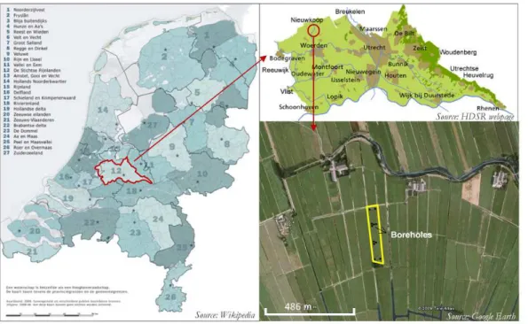
2 Research site

The research site was located at an experimental field in the Zegvelderbroek polder at approximately 2.5 km north of Zegveld, a small town in the province of Utrecht (Fig. 1). The site has the form of a parcel of land which is completely surrounded by ditches, and it has a surface area of 1.57 ha. The topography is very flat with land surface 5

elevations averaging around−2.30 m below sea level. The grass covered soils receive a mean precipitation of 826 mm yr−1 _{and the potential mean evapotranspiration has}

been estimated at around 545 mm yr−1

. The precipitation surplus of about 280 mm yr−1

is recharging the shallow groundwater.

The CCL in the area is part of the Holocene layer. This CCL has a thickness of 10

approximately 6 to 7 m. The lithology of the CCL is mainly dominated by peaty and clayey deposits which were deposited in an environment with slow moving mean-dering rivers where the peat grew in still waters at considerable distances from the main water courses and the clays originated from flood depositions. Clays of a ma-rine origin are also present. Sand deposits occur as well and can be related to bed 15

deposits of the ancient water courses. The Pleistocene below the Holocene consists of medium to coarse sandy deposits of considerable thickness (around 18 m). According to Bierkens (1994) and Weerts (1996) these sandy deposits, also referred to as the Kreftenheye Formation, were deposited during the Weichselian ice age and originated from braided river systems.

20

The research site is part of an area consisting of an extended network of ditches and canals to drain the polder areas in the winter season and to provide high groundwater tables during the dry summer. Thus, there is a strong interconnection between the groundwater and surface water. The organization responsible for water management in the area is the Water Board named Hoogheemraadschap de Stichtse Rijnlanden 25

(6)

HESSD

8, 2065–2101, 2011

P. Trambauer et al.

Title Page

Tables Figures

◭ ◮

Back Close

Full Screen / Esc

Discussion

P

a

per

|

Dis

cussion

P

a

per

|

Discussion

P

a

per

|

Discussio

n

P

a

per

|

3 Field and laboratory work

To investigate the heterogeneity and anisotropy and the applicability of Darcy’s law in groundwater flow modeling, a fieldwork program was defined and took place during the winter of 2009 to 2010. The fieldwork included drilling of two boreholes, about 150 m apart, through the CCL using a hand auger. Detailed sample descriptions of the col-5

lected soils were completed in the field. In addition, a geophysical survey was carried out in order to have more information on the aerial consistency of the layering detected during borehole drilling. The vertical electrical sounding (VES) method following the Schlumberger electrode layout was used.

Furthermore, slug tests were completed in 8 shallow boreholes to verify whether 10

the hydraulic conductivity in the peat layers is constant or varies with the imposed hydraulic gradient. Through laboratory tests, the relation between the variability of the hydraulic conductivity and the decomposition degree of the peat layers would also be established. In the boreholes used for the slug tests peat samples were taken at different depths and the decomposition degree was determined according to the von 15

Post method, the extracted carbon analysis technique and through the measurement of the absorbance (Price et al., 2005; Wang et al., 2004; Klavins et al., 2008).

Finally, time series of the groundwater levels were collected. The two boreholes penetrating through the CCL were equipped with piezometers. Other holes drilled up to the groundwater table and until halfway the CCL obtained piezometers as well. 20

(7)

HESSD

8, 2065–2101, 2011

P. Trambauer et al.

Title Page

Tables Figures

◭ ◮

Back Close

Full Screen / Esc

Discussion

P

a

per

|

Dis

cussion

P

a

per

|

Discussion

P

a

per

|

Discussio

n

P

a

per

|

4 Interpretation

4.1 Results of the field investigations

The soil descriptions showed a top layer of clayey and silty peat of around 1.5 m thick-ness. Below this layer the CCL consisted mainly of a highly moisturized, muddy ma-terial mixed with peat. In some places a lot of wood was present (Fig. 2). There were 5

localized places where only peat was found. Below the mud layer, a peat layer mixed with mud and some wood was observed. Near the 5 m depth mark, a thin layer of clay was located in one of the boreholes, below a layer that consisted of a mixture of clay with peat (humic clay). At the depth of 6.3 to 6.5 m the sandy Pleistocene aquifer was found.

10

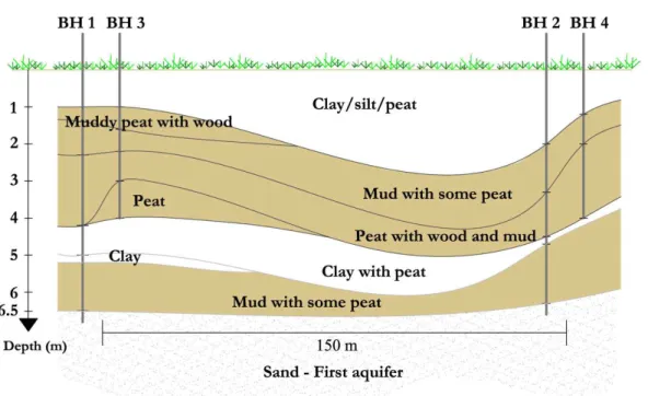
A cross sectional view through the CCL based on the soil descriptions at the two sites with both deeper and shallower boreholes indicates a continuity in lithology for most layers whereby the differences in layer thickness should be noted (see Fig. 3). However, not all the layers were found to be continuous as is demonstrated by the soil description of borehole 1, which had a muddy peat layer below the first layer that 15

was not present at borehole 2. Underpinning this discontinuity is the isolated layer of peat detected in borehole 3 and the thin layer of clay that was observed in borehole 1. These layers are faded out at borehole 2. The substantial changes in lithology in the vertical direction and the discontinuity of layers in a lateral sense prove that the CCL is truly a very heterogeneous unit.

20

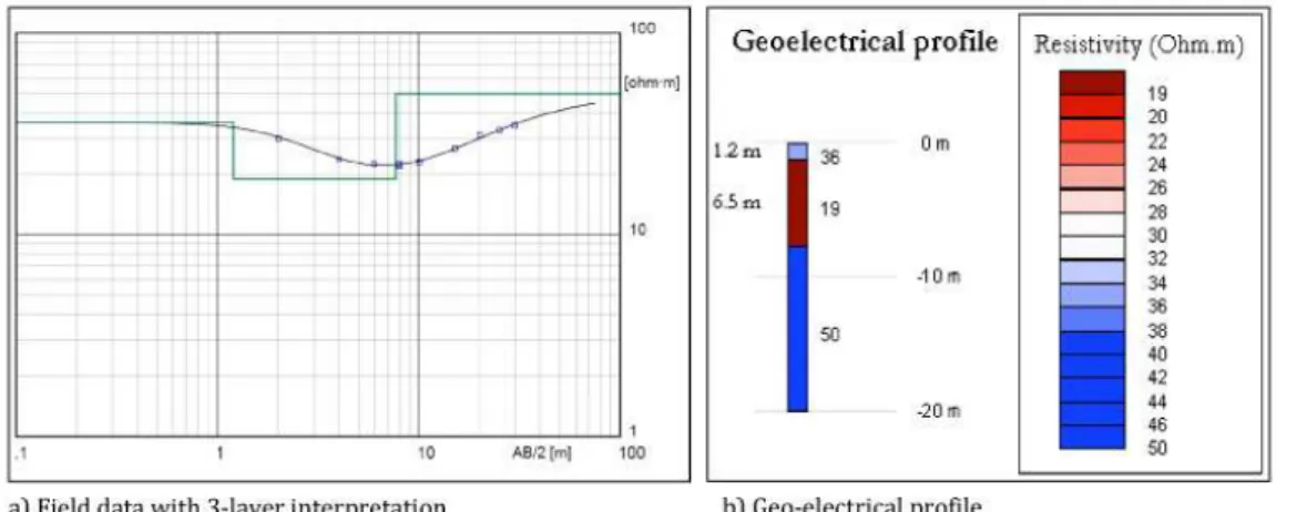
The geophysical VES measurement completed at the research site attained an in-vestigation depth of about 20 m which is well into the sandy Pleistocene aquifer. The interpretation of the measurement allowed a 2-layer schematization of the CCL indi-cating layer thicknesses of 1.2 m and 6.5 m (see Fig. 4). These layers are thought to coincide with the first clayey/silty peat layer and the underlying mud and peat layer. 25

(8)

HESSD

8, 2065–2101, 2011

P. Trambauer et al.

Title Page

Tables Figures

◭ ◮

Back Close

Full Screen / Esc

Discussion

P

a

per

|

Dis

cussion

P

a

per

|

Discussion

P

a

per

|

Discussio

n

P

a

per

|

apparently small, which did not allow the interpretation of more layers. The third layer found in the measurement represents the sandy Pleistocene deposits. The VES in-terpretation shows that at this location in the middle of the research site the general lithological built up of the CCL is similar to the sites where the boreholes allowed a detailed layer description.

5

4.2 Validity of Darcy’s law

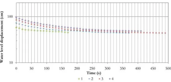
The slug tests carried out at the research site to test the applicability of Darcy’s law were first analyzed following methods based on steady state groundwater flow assuming a rigid system and negligible e_ffects on the water table. The van Beers (1963) approach and the Hvorslev’s method as suggested by Surridge et al. (2005) were selected. The 10

steady state formula as formulated by Surridge can be expressed as follows:

Kh=−A F tln

_h t h0

(1)

whereKhindicates the horizontal hydraulic conductivity (m d− 1

),tis time (d),h_t(m) and h0 (m) are respectively the head differences, caused by the removal of water, at time t and at the start of the test. TheAand F are geometrical factors. Head di_fferences 15

are vertical distances measured between water levels during the test in the hole and the static water level in the soil. The formula shows that a plot of ln (h_t/h0) against t produces a straight line since the other parameters in the expression are assumed to be constant.

Plots of ln (h_t/h0) or level displacement against t for the research site do not pro-20

(9)

HESSD

8, 2065–2101, 2011

P. Trambauer et al.

Title Page

Tables Figures

◭ ◮

Back Close

Full Screen / Esc

Discussion

P

a

per

|

Dis

cussion

P

a

per

|

Discussion

P

a

per

|

Discussio

n

P

a

per

|

Rather than contributing the phenomena to the non-applicability of Darcy’s law, the “curved line behavior” could be attributed to the peat not being a rigid framework for groundwater flow. Peat is compressible and therefore a transient behavior of the soil can be expected during slug tests. The use of the traditional steady state formula should be avoided (Hinsby et al., 1992; Surridge et al., 2005) and instead transient 5

formula have to be applied. Transient formulae to interpret slug tests in unconfined aquifers are hardly described in literature, but the KGS approach (Choi et al., 2008; Esling and Keller, 2009) and the Dax expression as suggested by Hinsby et al. (1992) can be considered.

The KGS approach is based on a semi-analytical model to estimate the storativity 10

and the hydraulic conductivity of an unconfined aquifer for the transient situation. Dax simplified and approximated the transient Cooper method used for fully screened wells in confined aquifers for partially penetrating wells and applied this method to uncon-fined aquifers with delayed yield, assuming horizontal radial flow to the well. The Dax expression can be described as follows:

15

Kh=

r_c2·ln Ho/Ht

L·t·D(α)

(2)

whereKhis the horizontal conductivity (m d− 1

),tis time (d), andH_t(m) andH0(m) are head di_fferences, following the injection of water, at timet and at the start of the test. ThercandLare geo-metrical factors, and theD(α) is a variable also containing timet. TheD(α) includes a term for the storativityS of the soil which represents the capacity 20

for elastic storage depending on the compressibility of the material (Hinsby, 1992). The Scan be obtained using the Cooper method when the unconfined aquifer is showing a delayed yield response.

Using steady state and transient formulae,Khvalues were computed for the 8 shal-low boreholes using a spreadsheet (Table 1). Level displacement against timet plots 25

(10)

HESSD

8, 2065–2101, 2011

P. Trambauer et al.

Title Page

Tables Figures

◭ ◮

Back Close

Full Screen / Esc

Discussion

P

a

per

|

Dis

cussion

P

a

per

|

Discussion

P

a

per

|

Discussio

n

P

a

per

|

indicating sites where the soil material was apparently more rigid. The tests producing “curved lines” have been interpreted using the transient KGS and Dax methods, but for comparative reasons have also been analyzed using the steady-state van Beers and Hvorslev methods. The computed Kh values fall within the range of 0.1 to 1.6 m d−

1

which are normal values for peat land areas in The Netherlands (Weerts, 1996). The 5

consistently lower values obtained with the KGS approach in relation to the Dax method may be due to the difficulty in determining accurateS values for the latter method.

A comparison can be made between the obtainedKh values, the compressibility at the site and the decomposition degree of the peat. The latter can be expressed using the von Post scale. The bore holes with higher conductivities and a higher compress-10

ibility interpreted with the transient KGS and Dax methods have a higher decomposition degree (Table 1: BH 5, 6, 9, 11, 12). Typically, these slug tests were carried out in well decomposed peat which has a muddy and plastic appearance containing besides peat also mineral components. The holes with lower conductivities and a more rigid soil analyzed with the steady state van Beers and Hvorslev formula have a relatively low 15

decomposition degree (BH 7, 8, 10). These tests were carried out in more coherent soils made up of clay, silt and peat or where fresh, largely intact peat was found.

The inappropriate use of steady-state formula to interpret slug tests in compressible peat has led wrongly to the believe that Darcy’s law is not valid in these types of mate-rials, but on the other hand full prove has also not been given that this most important 20

law for groundwater can really be applied in peaty environments. In other words, is the hydraulic conductivityKhreally independent of the hydraulic gradient or hydraulic head differences in the groundwater flow system? Waine et al. (1985) presented evidence of a higher hydraulic conductivity of well-decomposed peats with an increase in hydraulic gradient for steady-state experiments set up in the laboratory. However, the effect of 25

(11)

HESSD

8, 2065–2101, 2011

P. Trambauer et al.

Title Page

Tables Figures

◭ ◮

Back Close

Full Screen / Esc

Discussion

P

a

per

|

Dis

cussion

P

a

per

|

Discussion

P

a

per

|

Discussio

n

P

a

per

|

differences applied. Based on this information one is inclined to believe that Darcy’s law with a constantKhmay not be entirely valid to describe groundwater flow in peaty environments, but that its application in analytical and numerical model computations is justified.

5 Modeling results

5

The groundwater modeling at the research site incorporates the heterogeneities of the Complex Confining Layer (CCL) which were disclosed from the fieldwork. The mod-eling results have been compared with the outcome of a simplified model whereby the CCL is represented as a single homogeneous layer. In this way the effect of het-erogeneity on modeling results has been established. For the comparison calibrated 10

models have been used keeping in mind the limitations attached to model verification following standard rules for model calibration (Konikow and Bredehoeft, 1992).

5.1 Conceptual model

5.1.1 Layer schematization

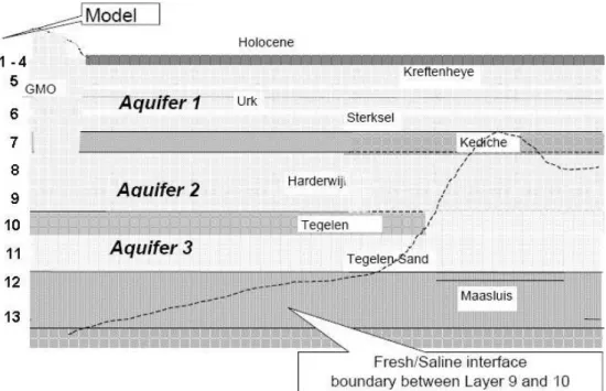
The heterogeneities in the CCL made it clear that a one layer schematization of the 15

CCL is too simplified and at least a distinction has to be made between the muddy and peaty layers and the more clayey layers. Based on the cross section obtained from the drilling activities (Fig. 3), the schematization of the CCL in the model area included a representation by 4 model layers (Fig. 6). The alteration of sandy aquifers and clayey aquitards below the CCL were represented by another 9 model layers bringing the total 20

(12)

HESSD

8, 2065–2101, 2011

P. Trambauer et al.

Title Page

Tables Figures

◭ ◮

Back Close

Full Screen / Esc

Discussion

P

a

per

|

Dis

cussion

P

a

per

|

Discussion

P

a

per

|

Discussio

n

P

a

per

|

5.1.2 Boundary conditions

The groundwater model was not confined to the boundaries of the actual research site which measures 50 m by 300 m but was considerably larger having a size of 700 m by 900 m. At the boundaries groundwater level-controlled conditions were assumed for all the model layers. The selection of a larger model area than the research site can be 5

explained by the introduction of errors at the boundaries. Measurement-based ground-water levels assigned to the boundaries will contain measurement and interpolation errors which will affect the model results especially at the margins of the model and less in the centrally located research site.

5.1.3 Groundwater balance

10

A groundwater balance can be defined for the entire model area including all model layers. The focus of attention in this paper is on the CCL and therefore the balance for this confining layer has been introduced as follows:

(Qprec−Qcap)+(Qsurf-in−Qsurf-out)+(Qup−Qdown)= ∆VCCL

∆t (3)

whereQprec (m 3

d−1_{) denotes the recharge at the groundwater table in the CCL as a}

15

result of precipitation,Qcap (m 3

d−1

) expresses the capillary rise from the table, Qsurf-in andQsurf-out(m

3

d−1_{) refer to respectively the groundwater inflow and the outflow at the}

ditches, and theQup and Qdown (m 3

d−1

) are the vertical upward and downward flow exchanges between the CCL and underlying Pleistocene sandy aquifer. The term∆ VCCL/∆t (m

3

d−1_{) describes the change in water storage per time step}

∆t in the CCL. 20

(13)

HESSD

8, 2065–2101, 2011

P. Trambauer et al.

Title Page

Tables Figures

◭ ◮

Back Close

Full Screen / Esc

Discussion

P

a

per

|

Dis

cussion

P

a

per

|

Discussion

P

a

per

|

Discussio

n

P

a

per

|

5.2 Model code and data input

The selected code for the modeling at the research site was the well-known package PMWIN-MODFLOW which is based on Darcy’s law. The grid for the MODFLOW model was designed with a constant cell size of 5 m by 5 m. This relatively small cell size relates to the small width of 50 m of the parcel of grass land forming the research site. 5

In order to compute and calibrate the groundwater levels in this parcel bounded by ditches with su_fficient accuracy, this small cell resolution was required.

5.2.1 Hydro-geological parameters

A Digital Elevation Model (DEM) with a resolution of 5 m by 5 m provided the information to input into the model the elevations of the land surface which varied between−1.9 10

up to 2.7 m below sea level. Based on fieldwork data, the elevations (of the top and bottom) of the model layers making up the CCL were inserted into the model. The bottom of the CCL varies between−8.4 m and 9.1 m below sea level. Borehole data of the database residing with the Institute of Applied Sciences (TNO) were interpolated to obtain adequate elevations of the model layers, corresponding with the sandy aquifers 15

and clayey aquitards below the CCL.

Slug test experiments carried out during the fieldwork, permeameter laboratory tests completed by the Wageningen University and Research Centre, different literatures that discuss the permeability of the CCL (e.g. Weerts, 1996), and pumping tests carried out in nearby pumping stations for domestic water supply were considered in providing 20

(14)

HESSD

8, 2065–2101, 2011

P. Trambauer et al.

Title Page

Tables Figures

◭ ◮

Back Close

Full Screen / Esc

Discussion

P

a

per

|

Dis

cussion

P

a

per

|

Discussion

P

a

per

|

Discussio

n

P

a

per

|

5.2.2 Time and model boundary levels

Steady state and transient models were prepared for specific periods. The steady state model runs on the input of data for the year 1990. This year reflects average meteorological conditions and the model simulates average groundwater levels and flows (Cheng, 2004). The transient model was initially built for the input of 10-day 5

averaged data for the winter period 2009 to 2010, but was extended at a later stage to simulate 4 and 8 yr simulation periods from either from 2002 or 2006 up to the spring of 2010. The extension was necessary in order to visualize the complete pathlines of water particles through the CCL and to be able to compute corresponding travel times. Field-based measurements defined the boundary- and initial groundwater levels for 10

the active modeling area. For the peaty layers with a phreatic response in the CCL the levels, ranging from−2.3 to 2.9 m below sea level, were obtained from so called GxG maps. The phreatic surface, which is rather irregular in the ditch and land parcel land-scape of the model area, has been taken from these high resolution groundwater level maps. For the Pleistocene sandy aquifer and the deeper aquifers, the TNO database 15

provided the levels for the model. The levels covered the range from −2.9 to 3.9 m below sea level. Since piezometric surfaces of the sandy aquifers are rather smooth, the levels for the model boundaries could reliably be estimated by interpolation of data available for the few boreholes present in the area.

5.2.3 Groundwater recharge and the surface water system

20

An unsaturated model for the root zone supplied the input data for groundwater recharge from precipitation. This model considering as main input parameters soil characteristics, precipitation and potential evapotranspiration, computes net recharge as the balance between downward recharge and capillary rise. Precipitation data for the rainfall station at the research area itself and evapotranspiration data from the De 25

(15)

HESSD

8, 2065–2101, 2011

P. Trambauer et al.

Title Page

Tables Figures

◭ ◮

Back Close

Full Screen / Esc

Discussion

P

a

per

|

Dis

cussion

P

a

per

|

Discussion

P

a

per

|

Discussio

n

P

a

per

|

period selected for the steady model, the computed net recharge varied from a high of 2.3 mm d−1 _{to a low of}

−1.7 mm d−1 yielding a realistic average recharge value of 0.41 mm d−1_{as model input.}

The Water Board HDSR provided surface water information including data relating to the River Oude Meije and the extensive ditch system. The data comprise river and 5

ditch characteristics like bed hydraulic conductances, open water levels and elevations of the bottom of these surface water courses. The open water levels at the river and ditches in the model area are controlled by HDSR and maintained at a fixed position for winter and summer conditions.

5.3 Sensitivity analysis and model calibration

10

The data input for the models was followed by a sensitivity analysis aiming to identify the parameters which have a large effect on modeling results including the computed phreatic and piezometric groundwater levels. The analysis showed that increases or decreases of 50% in the values for the hydraulic conductivity of the CCL and the groundwater recharge resulted in phreatic groundwater level changes of less than 15

0.1 m and piezometric groundwater level changes were even below 0.01 m. The hy-draulic conductivity is a bit less sensitive than the recharge. The transient models require the input of storage parameters like the specific yield and this parameter is also sensitive. From a general point of view, however, the sensitivity of model parameters is not that large which could be attributed to the control which the open water levels at 20

the ditches exert on the groundwater levels.

Taking into account the results of the sensitivity analysis the models were calibrated which meant that parameter values were changed in order to try to minimize the diff er-ence between the groundwater levels computed with the model and the groundwater levels measured in the field. Although the hydraulic conductivities are less sensitive 25

(16)

HESSD

8, 2065–2101, 2011

P. Trambauer et al.

Title Page

Tables Figures

◭ ◮

Back Close

Full Screen / Esc

Discussion

P

a

per

|

Dis

cussion

P

a

per

|

Discussion

P

a

per

|

Discussio

n

P

a

per

|

than the values for the recharge. During the actual calibration work with the steady state model the phreatic groundwater levels computed on the bases of a particular set of parameter values were compared with the field-based phreatic levels shown on the GxG maps. For the transient model computed phreatic and piezometric groundwater levels could be compared with groundwater levels measured during the fieldwork in 5

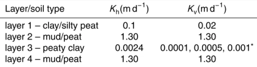
the upper peaty layers of the CCL and in the sandy first aquifer. Model calibration resulted, for final mean absolute differences in computed and measured groundwater levels of less than 0.05 m, in particular in upgraded model conductivities ranging from 0.0001 m d−1 _{for the clayey parts of the CCL up to 1.3 m d}−1 _{for the peaty layers (see}

Table 2). 10

5.4 Comparison of detailed and simplified models

Results of the calibrated detailed models with a heterogeneous CCL were compared with the outcomes of simplified models whereby the CCL is represented as a sin-gle homogeneous layer. To obtain a representative simplified model the upper four layers of the detailed model were merged into a single layer with equivalent values 15

for parameters including the hydraulic conductivities and the effective porosity. The equivalent value for the horizontal conductivity was obtained from the total horizon-tal transmissivity of the CCL and was calculated asKh=0.961 m d−

1

. The equivalent vertical conductivity was elaborated from the total resistance across the CCL. Some aerial variation in resistance had to be taken into account leading to the computation 20

of equivalent values with magnitudes of Kv1=0.0114 m d− 1

, Kv2=0.0061 m d− 1

and Kv3=0.0013 m d−

1

. For the equivalent porosity an average of the 4 model layers of 0.26 was considered. The assignment of equivalent values to the simplified model means that the unique effect of heterogeneity can properly be determined when com-paring model results.

25

(17)

HESSD

8, 2065–2101, 2011

P. Trambauer et al.

Title Page

Tables Figures

◭ ◮

Back Close

Full Screen / Esc

Discussion

P

a

per

|

Dis

cussion

P

a

per

|

Discussion

P

a

per

|

Discussio

n

P

a

per

|

trajectories that water particles may have followed through the CCL and travel time computations indicate the time it takes a water particle to flow through the CCL to or from the sandy aquifer or the ditch system. In the peat areas in the western part of The Netherlands the dominant flow of the water particles may be either downward or upward. The prepared detailed and simplified models for the research area are 5

representative for areas where groundwater flow is primarily directed in a downward direction. Additional hypothetical models have been prepared to study the path lines and travel times for typical upward flow through the CCL.

5.4.1 Typical downward flow through the CCL

Steady state model

10

Steady state models for the research area have been used to obtain pathlines and travel times for the typical case of downward flow through the CCL. The models as-sume that average hydrological conditions are maintained over a long time. The model results show that for both the heterogeneous and homogeneous cases the flow path of water particles are similar and the direction is almost vertically downward (Figs. 8 and 15

9). When the particles arrive in the sandy aquifer the flow becomes more horizontal. For the heterogeneous case the travel time of water through the saturated CCL was approximately 7 yr and for the homogeneous case a water particle was underway in the CCL for 9 yr. The longer travel time for the homogeneous case could be explained by the use of equivalent values for the hydraulic conductivities and effective porosities 20

which influence the head distribution and affect the travel time in the CCL.

Transient model

(18)

HESSD

8, 2065–2101, 2011

P. Trambauer et al.

Title Page

Tables Figures

◭ ◮

Back Close

Full Screen / Esc

Discussion

P

a

per

|

Dis

cussion

P

a

per

|

Discussion

P

a

per

|

Discussio

n

P

a

per

|

pathline trajectories and travel times than the steady state model. The model outcomes emphasize that the flowpath of a water particle is directed downward (Figs. 10 and 11). However, in the heterogeneous case there is a larger tendency of a particle, entering the saturated CCL in spring, to end up in the ditch then for the homogeneous set up. This has to do with the smaller velocities in the first clayey model layer for the heteroge-5

neous case during the subsequent summer period when the flow exchange is from the ditch into the CCL. The particles are kept “within reach” of the ditches and may actually discharge into them through the second peaty model layer during the following winter season. Water particles entering in the autumn period may show an opposite behavior and would tend to end up less in the ditches in the heterogeneous model than in the 10

homogeneous case.

Confirming the results of the steady state model, the travel times calculated for the heterogeneous case are shorter than for the homogeneous model set up. For the former case the travel time through the saturated CCL is in the order of 4 yr and for the latter case the water particles have not even reached half way through the covering 15

layer in this period. The travel times for the transient models are also less than for the steady models indicating that the differences in head distributions between the models play a prominent role. These differences can be attributed to the average hydrological conditions and constant water levels assumed for the steady simulation and the seasonally varying conditions and levels adopted for the transient state. 20

5.4.2 Typical upward flow through the CCL

Transient hypothetical models have been used to generate pathline patterns and com-pute travel times for upward flow through the CCL. For comparative reasons, the ab-solute differences in phreatic and piezometric groundwater levels for the models were similar than for the models simulating downward flow. To visualize the flow through 25

(19)

HESSD

8, 2065–2101, 2011

P. Trambauer et al.

Title Page

Tables Figures

◭ ◮

Back Close

Full Screen / Esc

Discussion

P

a

per

|

Dis

cussion

P

a

per

|

Discussion

P

a

per

|

Discussio

n

P

a

per

|

culminating in a prominent outflow at the ditches (Figs. 12 and 13). Although upward flow is dominant also downward flow exists in the upper parts of the CCL. The het-erogeneous case also clearly shows in the second peaty model layer and centrally between the ditches, the development of an area with nearly stagnant groundwater flow.

5

The travel times calculated for upward flow are comparable with those for downward flow. For the heterogeneous case the travel time for a water particle to move from the sandy aquifer into the ditch is in the order of 2 to 4 yr and when homogeneous conditions are considered the travel time to the ditch is longer, ranging from 5 to 8 yr. Not surprisingly, the travel times are shortest for particles that move upward in the CCL 10

below the ditches. Particles that flow upward centrally between the ditches where the stagnant area is located take the longest time to finally reach the surface water system.

6 Conclusions

The shallow surface- and groundwater system in a typical peat lowland area in The Netherlands could successfully be analysed using a combination of fieldwork and mod-15

eling work. Uncertainties in modeling arising from the heterogeneity in peat soils and the applicability of Darcy’s law could be eliminated through a proper model set up. The model itself provided useful information on the flowpath patterns and travel times of groundwater through the Complex Confining Layer (CCL) and the flow exchange with the ditch system.

20

The fieldwork and previous investigations (e.g. Weerts, 1996) indicated that the CCL indeed deserves its reputation of being a very complex layer. Borehole drilling revealed that both in the vertical and horizontal direction the CCL is heterogeneous. In the vertical direction layers of peaty and silty clay, mud and peat, clay and again peat succeed each other in a downward direction at the research site. The CCL rests on 25

(20)

HESSD

8, 2065–2101, 2011

P. Trambauer et al.

Title Page

Tables Figures

◭ ◮

Back Close

Full Screen / Esc

Discussion

P

a

per

|

Dis

cussion

P

a

per

|

Discussion

P

a

per

|

Discussio

n

P

a

per

|

horizontal direction the various layers are continuous in many places, but also tend to wedge out offering additional complexity for groundwater flow.

Field slug tests indicated that an apparent variable Kh was observed for humified peat soils but this is thought to be due to the inappropriate use of steady state formula for transient experiments. Even though these expressions are normally used for tran-5

sient slug tests, they were found to be inappropriate for this kind of peat soils. During the tests the humified peat soils introduce a large transient effect as a result of the compressibility of the peat and its plastic nature. On the other hand, the slug tests gave no clear evidence of the dependency of the hydraulic conductivity with the hy-draulic gradient. In combination with earlier results from laboratory tests (Waine et al., 10

1985), the evidences proved that changes in the hydraulic gradient hardly affect the hydraulic conductivity and, therefore, Darcy’s law can be used for peat soils. Based on interpreted elastic storativity values of the peat, varying from 0.0001 to 0.001, the hydraulic conductivity of the humified peat soil could be computed with an equation for transient conditions and a semi-analytical model yielding values in the range of 0.24 15

and 1.69 m d−1_.

The modeling work focused on the comparison of a detailed model for the peaty CCL and a model with aggregated parameters. The detailed model takes into account the heterogeneity of the CCL which is represented by 4 model layers and the aggre-gated model considers the CCL as an apparent homogeneous entity. The transient 20

models run for an 8 yr simulation period proved to be adequate to visualize the pathline patterns in the CCL for downward flow in the research area and for upward flow en-countered in other similar areas in the western part of The Netherlands. As a result of the similar hydrological conditions adopted at the boundaries of the CCL the flow line patterns for the model representing the heterogeneous case are quite similar to those 25

(21)

HESSD

8, 2065–2101, 2011

P. Trambauer et al.

Title Page

Tables Figures

◭ ◮

Back Close

Full Screen / Esc

Discussion

P

a

per

|

Dis

cussion

P

a

per

|

Discussion

P

a

per

|

Discussio

n

P

a

per

|

An interesting result from the modeling exercises are the indications of the travel times of water particles when flowing through the peaty CCL. In case the heterogene-ity of the CCL is taken into account, the model computes travel times of water particles through the CCL which are considerably shorter than for the case whereby the Com-plex Confining Layer is represented by a single homogeneous model layer. Travel times 5

downward or upward through the CCL for the heterogeneous model range between 2 to 4 yr whereas the model with homogeneity tends to compute times in the order 5 to 8 yr. The conclusion is that groundwater models that are based on the representation of the CCL with one homogeneous model layer are less suitable for assessments on groundwater transport where travel times play an important role. In particular when 10

they are considered for the simulation of contaminant transport, models with a homo-geneous CCL should not be used.

Acknowledgements. We gratefully acknowledge the Water Board Hoogheemraadschap De Stichtse Rijnlanden for their financial support and the gathering of parts of the data presented in this research.

15

References

Bierkens, M. F. P.: Complex confining layers – a stochastic analysis of hydraulic properties at various scales, Netherlands geographical studies, 184, KNAG/Faculty of Geosciences, Utrecht University, Utrecht, The Netherlands, 272 pp., 1994.

Cheng, X.: Modelling of groundwater salinization risk – case study of the western stichtse

20

rijnlanden area, the netherlands, Msc. thesis HH489, UNESCO-IHE, Delft, 2004.

Choi, H., Nguyen, T.-B., and Lee, C.: Slug test analysis to evaluate permeability of compressible materials, Ground Water, 46, 647–652, 2008.

Dufour, F. C.: Groundwater in the netherlands – facts and figures, Delft/Utrecht, The Nether-lands, 2000.

25

Esling, S. P. and Keller, J. E.: A user interface for the kansas geological survey slug test model, Ground Water, 47, 587–590, 2009.

(22)

HESSD

8, 2065–2101, 2011

P. Trambauer et al.

Title Page

Tables Figures

◭ ◮

Back Close

Full Screen / Esc

Discussion

P

a

per

|

Dis

cussion

P

a

per

|

Discussion

P

a

per

|

Discussio

n

P

a

per

|

for determination of a local hydraulic conductivity of an unconfined sandy aquifer, J. Hydrol., 136, 87–106, 1992.

Ingram, H. A. P., Rycroft, D. W., and Williams, D. J. A.: Anomalous transmission of water through certain peats, J. Hydrol., 22, 213–218, 1974.

Klavins, M., Sire, J., Purmalis, O., and Melecis, V.: Approaches to estimating humification

5

indicators for peat, Mires and Peat, 3, Article 7, 2008.

McDonald, M. G. and Harbaugh, A. W.: A modular three-dimensional finite difference ground-water flow model: US Geological survey techniques of ground-water resources investigations, US Geological Survey, Denver, Colorado, 586 pp., 1998.

Price, J. S., Cagampan, J., and Kellner, E.: Assessment of peat compressibility: Is there an

10

easy way?, Hydrol. Process., 19, 3469–3475, 2005.

Surridge, B. W. J., Baird, A. J., and Heathwaite, A. L.: Evaluating the quality of hydraulic conductivity estimates from piezometer slug tests in peat, Hydrol. Process., 19, 1227–1244, 2005.

van Beers, W. F. J.: The auger hole method: A field measurement of the hydraulic conductivity

15

of soil below the water table, H. Veenman & Zonen, Wageningen, The Netherlands, 31 pp., 1963.

Waine, J., Brown, J. M. B., and Ingram, H. A. P.: Non-darcian transmission of water in certain humified peats, J. Hydrol., 82, 327–339, 1985.

Wang, H., Hong, Y., Zhu, Y., Hong, B., Lin, Q., Xu, H., Leng, X., and Mao, X.: Humification

20

degrees of peat in qinghai-xizang plateau and palaeoclimate change, Chinese Sci. Bull., 49, 514–519, 2004.

Weerts, H. J. T.: Complex confining layers – architecture and hydraulic properties of holocene and late weichselian deposits in the fluvial rhine-meuse delta, the netherlands, Netherlands geographical studies, 213, KNAG/Faculty of Geosciences, Utrecht University, Utrecht, The

25

(23)

HESSD

8, 2065–2101, 2011

P. Trambauer et al.

Title Page

Tables Figures

◭ ◮

Back Close

Full Screen / Esc

Discussion

P

a

per

|

Dis

cussion

P

a

per

|

Discussion

P

a

per

|

Discussio

n

P

a

per

|

Table 1.Horizontal hydraulic conductivityKh(m d− 1

) computed from the slug tests.

Borehole van Beers Hvorslev Dax KGS model Decomp Degree

∆t1 ∆t2 ∆t3 ∆t4 ∆t5 vPost

BH5 1.60 1.66 0.86 0.67 0.47 0.22 1.69 1.00 H7

BH6 0.72 0.70 0.57 1.34 0.73 H5

BH7 0.11 0.10 H4

BH8 0.27 0.26 H4

BH9 0.67 0.58 0.34 0.69 0.45 H6

BH10 0.15 0.15 H4

BH11 0.56 0.52 0.44 0.42 1.00 0.48 H6

(24)

HESSD

8, 2065–2101, 2011

P. Trambauer et al.

Title Page

Tables Figures

◭ ◮

Back Close

Full Screen / Esc

Discussion

P

a

per

|

Dis

cussion

P

a

per

|

Discussion

P

a

per

|

Discussio

n

P

a

per

|

Table 2. Horizontal and vertical hydraulic conductivities for the model layers representing the CCL.

Layer/soil type K_h(m d−1₎ _K v(m d−

1

) layer 1 – clay/silty peat 0.1 0.02 layer 2 – mud/peat 1.30 1.30

layer 3 – peaty clay 0.0024 0.0001, 0.0005, 0.001∗

layer 4 – mud/peat 1.30 1.30

(25)

HESSD

8, 2065–2101, 2011

P. Trambauer et al.

Title Page

Tables Figures

◭ ◮

Back Close

Full Screen / Esc

Discussion

P

a

per

|

Dis

cussion

P

a

per

|

Discussion

P

a

per

|

Discussio

n

P

a

per

|

(26)

HESSD

8, 2065–2101, 2011

P. Trambauer et al.

Title Page

Tables Figures

◭ ◮

Back Close

Full Screen / Esc

Discussion

P

a

per

|

Dis

cussion

P

a

per

|

Discussion

P

a

per

|

Discussio

n

P

a

per

|

(27)

HESSD

8, 2065–2101, 2011

P. Trambauer et al.

Title Page

Tables Figures

◭ ◮

Back Close

Full Screen / Esc

Discussion

P

a

per

|

Dis

cussion

P

a

per

|

Discussion

P

a

per

|

Discussio

n

P

a

per

|

(28)

HESSD

8, 2065–2101, 2011

P. Trambauer et al.

Title Page

Tables Figures

◭ ◮

Back Close

Full Screen / Esc

Discussion

P

a

per

|

Dis

cussion

P

a

per

|

Discussion

P

a

per

|

Discussio

n

P

a

per

|

(29)

HESSD

8, 2065–2101, 2011

P. Trambauer et al.

Title Page

Tables Figures

◭ ◮

Back Close

Full Screen / Esc

Discussion

P

a

per

|

Dis

cussion

P

a

per

|

Discussion

P

a

per

|

Discussio

n

P

a

per

|

(30)

HESSD

8, 2065–2101, 2011

P. Trambauer et al.

Title Page

Tables Figures

◭ ◮

Back Close

Full Screen / Esc

Discussion

P

a

per

|

Dis

cussion

P

a

per

|

Discussion

P

a

per

|

Discussio

n

P

a

per

|

(31)

HESSD

8, 2065–2101, 2011

P. Trambauer et al.

Title Page

Tables Figures

◭ ◮

Back Close

Full Screen / Esc

Discussion

P

a

per

|

Dis

cussion

P

a

per

|

Discussion

P

a

per

|

Discussio

n

P

a

per

|

(32)

HESSD

8, 2065–2101, 2011

P. Trambauer et al.

Title Page

Tables Figures

◭ ◮

Back Close

Full Screen / Esc

Discussion

P

a

per

|

Dis

cussion

P

a

per

|

Discussion

P

a

per

|

Discussio

n

P

a

per

|

(33)

HESSD

8, 2065–2101, 2011

P. Trambauer et al.

Title Page

Tables Figures

◭ ◮

Back Close

Full Screen / Esc

Discussion

P

a

per

|

Dis

cussion

P

a

per

|

Discussion

P

a

per

|

Discussio

n

P

a

per

|

(34)

HESSD

8, 2065–2101, 2011

P. Trambauer et al.

Title Page

Tables Figures

◭ ◮

Back Close

Full Screen / Esc

Discussion

P

a

per

|

Dis

cussion

P

a

per

|

Discussion

P

a

per

|

Discussio

n

P

a

per

|

(35)

HESSD

8, 2065–2101, 2011

P. Trambauer et al.

Title Page

Tables Figures

◭ ◮

Back Close

Full Screen / Esc

Discussion

P

a

per

|

Dis

cussion

P

a

per

|

Discussion

P

a

per

|

Discussio

n

P

a

per

|

(36)

HESSD

8, 2065–2101, 2011

P. Trambauer et al.

Title Page

Tables Figures

◭ ◮

Back Close

Full Screen / Esc

Discussion

P

a

per

|

Dis

cussion

P

a

per

|

Discussion

P

a

per

|

Discussio

n

P

a

per

|

(37)

HESSD

8, 2065–2101, 2011

P. Trambauer et al.

Title Page

Tables Figures

◭ ◮

Back Close

Full Screen / Esc

Discussion

P

a

per

|

Dis

cussion

P

a

per

|

Discussion

P

a

per

|

Discussio

n

P

a

per

|