Neutral atmosphere temperature change at 90 km, 70° N, 19° E, 2003–2014

(1)

ACPD

15, 15289–15317, 2015

Neutral atmosphere temperature change at 90 km, 70◦_{N, 19}◦_E,

2003–2014

S. E. Holmen et al.

Title Page

Abstract Introduction

Conclusions References

Tables Figures

◭ ◮

Back Close

Full Screen / Esc

Printer-friendly Version Interactive Discussion

Discussion

P

a

per

|

Discussion

P

a

per

|

Discussion

P

a

per

|

Discussion

P

a

per

|

Atmos. Chem. Phys. Discuss., 15, 15289–15317, 2015 www.atmos-chem-phys-discuss.net/15/15289/2015/ doi:10.5194/acpd-15-15289-2015

This discussion paper is/has been under review for the journal Atmospheric Chemistry and Physics (ACP). Please refer to the corresponding final paper in ACP if available.

Neutral atmosphere temperature change

at 90 km, 70

◦

_{N, 19}

◦

_{E, 2003–2014}

S. E. Holmen1,2,3, C. M. Hall2, and M. Tsutsumi4,5

1

The University Centre in Svalbard, Longyearbyen, Norway

2

Tromsø Geophysical Observatory, UiT – The Arctic University of Norway, Tromsø, Norway

3

Birkeland Centre for Space Science, Bergen, Norway

4

National Institute of Polar Research, Tokyo, Japan

5

The Graduate University for Advanced Studies (SOKENDAI), Department of Polar Science, Hayama, Japan

Received: 28 April 2015 – Accepted: 12 May 2015 – Published: 5 June 2015

Correspondence to: S. E. Holmen ([email protected])

(2)

ACPD

15, 15289–15317, 2015

2003–2014

S. E. Holmen et al.

Title Page

Tables Figures

◭ ◮

Back Close

Full Screen / Esc

Discussion

P

a

per

|

Discussion

P

a

per

|

Discussion

P

a

per

|

Discussion

P

a

per

|

Abstract

Neutral temperatures for 90 km height above Tromsø, Norway, have been determined using ambipolar diﬀ_{usion coe}ﬃ_{cients calculated from meteor echo fading times using} the Nippon/Norway Tromsø Meteor Radar (NTMR). Daily temperature averages have been calculated from November 2003 to October 2014 and calibrated against temper-5

ature measurements from the Microwave Limb Sounder (MLS) on board Aura. The long-term trend of temperatures from the NTMR radar is investigated, and winter and summer seasons are looked at separately. Seasonal variation has been accounted for, as well as solar response, using the F10.7 cm flux as a proxy for solar activity. The long-term temperature trend from 2003 to 2014 is ₋3.6 K_±1.1 K decade−1_{, with summer}

10

and winter trends₋0.8 K_±2.9 K decade−1 and ₋8.1 K_±2.5 K decade−1, respectively. How well suited a meteor radar is for estimating neutral temperatures at 90 km using meteor trail echoes is discussed, and physical explanations behind a cooling trend are proposed.

1 Introduction 15

Temperature changes in the mesosphere and lower thermosphere (MLT) region due to both natural and anthropogenic variations cannot be assessed without understand-ing the dynamical, radiative and chemical couplunderstand-ings between the diﬀ_{erent atmospheric} layers. Processes responsible for heating and cooling in the MLT region are many. Absorption of UV by O3 and O2 causes heating, while CO2 causes strong radiative

20

cooling. Planetary waves (PWs) and gravity waves (GWs) break and deposit heat and momentum into the middle atmosphere and influence the mesospheric residual cir-culation, which is the summer-to-winter circulation in the mesosphere. Also, heat is transported through advection and adiabatic processes.

For decades, it has been generally accepted that increased anthropogenic emis-25

(3)

ACPD

15, 15289–15317, 2015

2003–2014

S. E. Holmen et al.

Title Page

Tables Figures

◭ ◮

Back Close

Full Screen / Esc

Discussion

P

a

per

|

Discussion

P

a

per

|

Discussion

P

a

per

|

Discussion

P

a

per

|

Manabe and Wetherald, 1975), and that these emissions are causing the mesosphere and thermosphere to cool (Akmaev and Fomichev, 2000; Roble and Dickinson, 1989). Akmaev and Fomichev (1998) reported, using a middle atmospheric model, that if CO₂ concentrations are doubled, temperatures will decrease by about 14 K at the stratopause, by about 10 K in the upper mesosphere and by 40–50 K in the thermo-5

sphere. Newer and more sophisticated models include important radiative and dynam-ical processes as well as interactive chemistries, and they predict that the cooling rate near the mesopause is less than previously expected. The thermal response in this region is strongly influenced by changes in dynamics, and some dynamical processes contribute to a warming which counteracts the cooling expected from greenhouse gas 10

emissions (Schmidt et al., 2006).

Even though the increasing concentration of greenhouse gases is generally ac-cepted to be the main driver, also other drivers of long-term changes and temperature trends exist, namely stratospheric ozone depletion, long-term changes of solar and ge-omagnetic activity, secular changes of the Earth’s magnetic field, long-term changes 15

of atmospheric circulation and mesospheric water vapour concentration (Laš_tovič_ka et al., 2012). The complexity of temperature trends in the MLT region and their causes act as motivation for studying these matters further.

In this paper, we investigate long-term trends of temperatures obtained from the NTMR radar, and we also look at summer and winter seasons separately. In Sect. 2, 20

specifications of the NTMR radar are given, and the theory behind the retrieval of tem-peratures using ambipolar diﬀ_{usion coe}ﬃ_{cients from meteor trail echoes is explained.} In Sect. 3, the method behind the calibration of NTMR temperatures against Aura MLS temperatures is explained. Section 4 treats the temperature trend analysis, including the correction for seasonal variation and solar response. The theory and underlying as-25

(4)

ACPD

15, 15289–15317, 2015

2003–2014

S. E. Holmen et al.

Title Page

Tables Figures

◭ ◮

Back Close

Full Screen / Esc

Discussion

P

a

per

|

Discussion

P

a

per

|

Discussion

P

a

per

|

Discussion

P

a

per

|

2 Instrumentation and data

The Nippon/Tromsø Meteor Radar (NTMR) is located at Ramfjordmoen near Tromsø, at 69.58◦N, 19.22◦E. It is operated 24 h a day, all year round. Measurements are available for more than 90 % of all days since the radar was first operative in November 2003. The meteor radar consists of one transmitter antenna and five receivers and is operating 5

at 30.25 MHz. It detects echoes from ionized trails from meteors, which appear when meteors enter and interact with the Earth’s neutral atmosphere in the MLT region. The ionized atoms from the meteors are thermalized, and the resulting trails expand in the radial direction mainly due to ambipolar diﬀ_{usion, which is di}ﬀ_{usion in plasma due to} interaction with the electric field. Underdense meteors, which are the ones used in this 10

study, have a plasma frequency that is lower than the frequency of the radar, which makes it possible for the radio wave from the radar to penetrate into the meteor trail and be scattered by each electron.

Echoes are detected from a region with a radius of approximately 50 km. The radar typically detects around 10 000 echoes day−1, of which around 200–600 echoes are de-15

tected per hour at the peak occurrence height of 90 km. The number of echoes detected per day allows for a 30 min resolution of temperature values. The intra-day periodicity in meteor detections by the NTMR radar is less pronounced than that of lower latitude stations and we do not anticipate tidally-induced bias regarding echo rates at specific tidal phases for daily averages. The height resolution and the range resolution are both 20

1 km. From the decay time of the radar signal we can derive ambipolar diﬀ_{usion coe}ﬃ -cients,D_a:

Da= λ2

16π2_τ (1)

(5)

ACPD

15, 15289–15317, 2015

2003–2014

S. E. Holmen et al.

Title Page

Tables Figures

◭ ◮

Back Close

Full Screen / Esc

Discussion

P

a

per

|

Discussion

P

a

per

|

Discussion

P

a

per

|

Discussion

P

a

per

|

pressure:

Da=6.39×10−2K0 T2

p (2)

wherepis pressure,T is temperature, and K₀is the zero-field reduced mobility factor of the ions in the trail. In this study we use the value for K0 of 2.4×10−

4

m2s−1V−1, in accordance with e.g. Holdsworth et al. (2006). Pressure values are derived from at-5

mospheric densities obtained from falling sphere measurements appropriate for 70◦_N,

combining those of Lübken and von Zahn (1991) and Lübken (1999), previously used by e.g. Holdsworth (2006) and Dyrland et al. (2010).

The NTMR radar is essentially identical to the Nippon/Norway Svalbard Meteor Radar (NSMR) located in Adventdalen on Spitsbergen at 78.33◦N, 16.00◦E. Fur-10

ther explanation of the radar and explanation of theories can be found in e.g. Hall et al. (2002, 2012), Cervera and Reid (2000) and McKinley (1961).

Calibration of temperatures derived from meteor echoes with an independent, co-inciding temperature series is necessary, according to previous studies (e.g. Hocking, 1999). Temperatures from the NSMR radar have been derived most recently by Dyrland 15

et al. (2010), employing a new calibration approach for the meteor radar temperatures, wherein temperature measurements from the Microwave Limb Sounder (MLS) on the Aura satellite were used instead of the previously used rotational hydroxyl and potas-sium lidar temperatures from ground-based optical instruments (Hall et al., 2006). Nei-ther ground-based optical observations nor lidar soundings are available for the time 20

period of interest or the location of the NTMR. In this study we therefore employ the same approach as Dyrland et al. (2010), using Aura MLS temperatures to calibrate the NTMR temperatures.

NASA’s EOS Aura satellite was launched 15 July 2004 and gives daily global cov-erage (between 82◦_{S and 82}◦_{N) with about 14.5 orbits per day. The MLS instrument}

25

(6)

ACPD

15, 15289–15317, 2015

2003–2014

S. E. Holmen et al.

Title Page

Tables Figures

◭ ◮

Back Close

Full Screen / Esc

Discussion

P

a

per

|

Discussion

P

a

per

|

Discussion

P

a

per

|

Discussion

P

a

per

|

measurements of atmospheric temperature, among others (NASA Jet Propulsion Lab-oratory). Aura MLS temperature data (version 03) were obtained for latitude 69.7◦N_± 5.0◦and longitude 19.0◦E_±10.0◦at pressure 0.001 hPa, corresponding to_∼90 km.

3 Calibration of NTMR temperatures

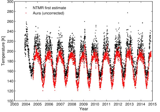
Figure 1 shows NTMR “raw” temperatures from November 2003 to October 2014, de-5

rived from Eqs. (1) and (2), plotted together with Aura MLS temperatures. The Aura satellite overpasses Tromsø at 01:00–03:00 and 10:00–12:00 UTC, which means that the Aura daily averages are representative for these time windows. It was therefore nec-essary to investigate any bias arising from Aura not measuring throughout the whole day. A way to do this is to assume that Aura temperatures and NTMR temperatures 10

follow the same diurnal variation and thus investigate the diurnal variation of NTMR temperatures. This was done by superposing all NTMR temperatures by time of day, obtaining 48 values for each day, since the radar allows for a 30 min resolution.

There is an ongoing investigation into the possibility thatDaderived by NTMR can be

aﬀ_{ected by modified electron mobility during auroral particle precipitation. According to} 15

Rees et al. (1972), neutral temperatures in the auroral zone show a positive correla-tion with geomagnetic activity. It is therefore a possibility that the diurnal variacorrela-tion of NTMR neutral temperatures is in fact influenced by aurora, and that apparentDa

en-hancements during strong auroral events do not necessarily depict neutral temperature increase. This matter requires further attention.

20

Investigation of possible unrealisticDaenhancements was carried out by calculating

standard errors of estimated half hourlyDavalues:

se= σ √

ne (3)

(7)

ACPD

15, 15289–15317, 2015

2003–2014

S. E. Holmen et al.

Title Page

Tables Figures

◭ ◮

Back Close

Full Screen / Esc

Discussion

P

a

per

|

Discussion

P

a

per

|

Discussion

P

a

per

|

Discussion

P

a

per

|

S. Nozawa (personal communication, 2015), all half hourlyDa values with a standard

error larger than 7 % of the estimated Da value were excluded from further analysis.

This rejection criterion led to that 5.4 % of theDavalues were rejected.

Figure 2 shows monthly averages of the superposed values of NTMR temperatures, after application of the Da rejection procedure, as a function of time of day for days

5

coinciding with Aura measurements. It is evident from the figure that the lowest tem-peratures are in general achieved in the forenoon, which coincides with one of the periods per day when Aura MLS makes measurements over Tromsø.

Subtracting the monthly averages of the 00:00–24:00 UTC temperatures from the 01:00–03:00 and 10:00–12:00 UTC temperatures gave the estimated biases in Aura 10

daily means due to only sampling during some hours of the day and are given in Fig. 3. The figure shows that by judging by the measurement windows, Aura underestimates the daily mean (00:00–24:00 UTC) more during winter that during spring and summer. Note the higher standard deviations in spring and summer compared to winter.

The initially obtained Aura temperatures were corrected by adding the biases from 15

Fig. 3 in order to arrive at daily mean temperatures that are representative for the entire day. Also, a 10 K correction for cold bias was applied to the Aura temperatures, following a suggestion from French and Mulligan (2010) from their comparison with other independent temperature measurements.

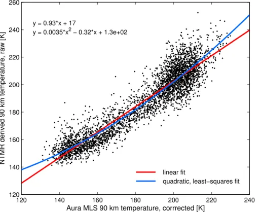
Figure 4 shows a scatterplot of the corrected Aura temperatures against the “raw” 20

NTMR temperatures. By observing the two datasets, a seasonally dependent relation-ship is discernible. A 2nd degree polynomial provided the best overall fit (R2=_0.87) compared with a linear fit. The blue line represents the quadratic, least-squares fit and is described by:

TNTMR=0.0035TAura2 −0.32TAura+126 (4)

25

whereTNTMRis the “raw” temperature obtained from NTMR, andTAura is the corrected

(8)

ACPD

15, 15289–15317, 2015

2003–2014

S. E. Holmen et al.

Title Page

Tables Figures

◭ ◮

Back Close

Full Screen / Esc

Discussion

P

a

per

|

Discussion

P

a

per

|

Discussion

P

a

per

|

Discussion

P

a

per

|

now corrected for the days of measurements coinciding with Aura measurements. For calibration of the remaining NTMR temperatures the same equation (Eq. 4) was used, with NTMR “raw” temperatures not coinciding with Aura measurements as input.

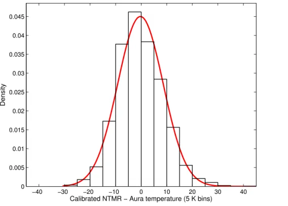
To estimate the calibration uncertainty, all corrected Aura temperatures were sub-tracted from the NTMR temperatures, and the diﬀ_{erences were plotted in a histogram} 5

with 5 K bins. A Gaussian was fitted to the distribution. The standard deviation of the Gaussian was 8.9 K, which is then considered the overall uncertainty of the calibra-tion. Figure 5 shows the histogram and the fitted Gaussian curve. Finally, Fig. 6 shows the calibrated NTMR temperatures with uncertainties plotted together with Aura MLS temperatures, corrected for tidal and cold bias.

10

4 Trend analysis

A monthly climatology of the calibrated NTMR temperatures was obtained by averaging all January, February, etc. values. The seasonal variation is shown in Fig. 7 and reveals a summer minimum of around 150–160 K and a winter maximum of around 200–210 K. The monthly values were then subtracted from the daily calibrated temperatures, ob-15

taining daily residuals independent of seasonal variation.

There are several measures of solar variability available, e.g. the F10.7 cm solar radio flux, the sunspot number (SSN), total solar irradiance (TSI), Mg II 280 nm core-to-wing ratio UV-index and the flare index (FI). These indices are considered proxies for solar radiation formed on diﬀ_{erent altitudes of the solar atmosphere and are highly} 20

correlated (Bruevich et al., 2014). In this study we use the F10.7 cm flux as a proxy for solar activity, which is the most commonly used index in middle/upper atmospheric temperature trend studies (e.g. Laš_tovič_{ka et al., 2008; Hall et al., 2012).}

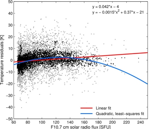
A 30 day running mean filter was applied to the daily residual temperatures. Figure 8 shows the residuals plotted against corresponding F10.7 cm values. The straight, red 25

(9)

ACPD

15, 15289–15317, 2015

2003–2014

S. E. Holmen et al.

Title Page

Tables Figures

◭ ◮

Back Close

Full Screen / Esc

Discussion

P

a

per

|

Discussion

P

a

per

|

Discussion

P

a

per

|

Discussion

P

a

per

|

applied and gave a solar response coeﬃ_{cient of 4.2 K}_±_{0.3 K (100 SFU)}−1 _{(1 SFU}= 1 solar flux unit=₁₀−22_{W m}−2_Hz−1_).

From Fig. 8 there appears to be a somewhat non-linear relationship between the tem-peratures at 90 km height and the F10.7 cm index. There seems to be a tendency of a less steep increase in temperatures toward higher F10.7 values. Ogawa et al. (2014) 5

also found a non-linear relationship between upper atmospheric temperatures and so-lar activity using EISCAT UHF radar observations from Tromsø, even though it must be noted that the altitude range they looked at diﬀ_{ers from ours. In Fig. 8 we have} there-fore also plotted the quadratic, least-squares fit to the running mean values. Lacking any objective scientific basis to do otherwise, we chose to fit a 2nd degree polynomial 10

following the philosophy of Ogawa et al. (2014), although it is conceivable that other functions could be more suitable. The 2nd degree polynomial gave us a better fit to the residuals (R2=_{0.17) compared to the straight line (}_R2=_{0.07). We subtracted the solar} response from the dataset of daily, seasonally corrected residuals using this relation:

T′=_T₋₍_a_·_f_10.72+_b_·_f_10.7+_c₎ ₍₅₎ 15

whereT′_{is the new set of residual temperatures with seasonal and solar response}

sub-tracted,T is the residual temperatures with only seasonal variation subtracted,f10.7 is the daily F10.7 cm flux corresponding toT, and a,band care coeﬃ_{cients of the 2nd} degree polynomial (a=₋_0.0015,_b=_0.37,_c=₋_21).

From the new set of temperature residuals we calculated monthly means. This was 20

done to remove any high-frequency deterministic component, such as that resulting from multi-day period waves. Finally, the linear trend was found by performing lin-ear regression using a least-squares fit. The long-term linlin-ear temperature trend us-ing monthly means is ₋3.6 K_±1.1 K decade−1. This trend can be considered statis-tically significant (i.e. significantly non-zero at the 5 % level), since the uncertainty 25

(10)

ACPD

15, 15289–15317, 2015

2003–2014

S. E. Holmen et al.

Title Page

Tables Figures

◭ ◮

Back Close

Full Screen / Esc

Discussion

P

a

per

|

Discussion

P

a

per

|

Discussion

P

a

per

|

Discussion

P

a

per

|

October 2014. For comparison, the long-term trend using daily temperature values is

−3.4 K±0.5 K decade−1.

In addition to the average temperature change, we also treated summer and win-ter seasons separately. First, trends for each month were investigated using the same approach as for the average regardless of month. Figure 10 shows the re-5

sult. Then, averages of November, December and January, and of May, June and July were made. They were defined as “winter” and “summer”, respectively. The long-term linear winter trend is₋8.1 K_±2.5 K decade−1, and the long-term summer trend is

−0.8 K±2.9 K decade−1.

The trend analysis was also performed without carrying out theD_a rejection proce-10

dure explained in Sect. 3. Final results with and without data rejection do not diﬀ_er significantly considering the calculated uncertainties.

5 Discussion

5.1 Suitability of a meteor radar for estimation of neutral temperatures at 90 km height

15

As explained in Sect. 2, neutral air temperatures derived from meteor trail echoes de-pend on pressure,p, the zero-field reduced mobility of the ions in the trail,K0, and

am-bipolar diﬀ_{usion coe}ﬃ_cients,_D

a.K0 will depend on the ion composition in the meteor

trail, as well as the chemical composition of the atmosphere. The chemical composition of the atmosphere is assumed to not change significantly with season (Hocking, 2004). 20

Unfortunately, the exact content of a meteor trail is unknown. Usually, a value forK₀

between 1.9_×10−4 and 2.9_×10−4m2s−1V−1 is chosen, depending on what ion one assumes to be the main ion of the trail (Hocking et al., 1997). Even though we in this study have chosen a constant value forK0of 2.4×10−

4

m2s−1_V−1_{, some variability in} K0is expected. According to Hocking (2004) variability can occur due to fragmentation

25

(11)

vari-ACPD

15, 15289–15317, 2015

2003–2014

S. E. Holmen et al.

Title Page

Tables Figures

◭ ◮

Back Close

Full Screen / Esc

Discussion

P

a

per

|

Discussion

P

a

per

|

Discussion

P

a

per

|

Discussion

P

a

per

|

ations in the composition of the meteor trail. Using computer simulations, they reported a typical variability inK0from meteor to meteor of 27 % and that the variability is most

dominant at higher temperatures. Based on this, we cannot rule out sources of error due to the choice ofK0as a constant, but since we have no possibility to analyse the

composition of all meteor trails detected by the radar we have no other choice than to 5

choose a constant value forK0.

How well ambipolar diff_{usion coe}ffi_{cients obtained for 90 km altitude are suited for} calculating neutral temperatures has previously been widely discussed, e.g. by Hall et al. (2012) for the trend analysis of the Svalbard meteor radar data, but will be shortly repeated here. For calculations of temperatures using meteor radar, ambipolar diff_usion 10

alone is assumed to determine the decay of the underdense echoes. Diff_{usivities are} expected to increase exponentially with height through the region from which meteor echoes are obtained (Ballinger et al., 2008; Chilson et al., 1996). Hall et al. (2005) found that this is only the case between_∼85 and_∼95 km altitude, using diff_{usion coe}ffi_cients delivered by NTMR from 2004. They found diff_{usivities less than expected above} _∼ 15

95 km and diﬀ_{usivities higher than expected below}_∼_{85 km. Ballinger et al. (2008) got} a similar result using meteor observations over northern Sweden. It has been proposed that processes other than ambipolar diﬀ_{usion influence meteor decay times. If this is} the case it may have consequences for the estimation of temperatures, and therefore it is important to investigate this further.

20

Departures of the anticipated exponential increase with height of molecular diﬀ u-sion above_∼95 km have in previous studies been attributed to gradient-drift Farley– Buneman instability. Farley–Buneman instability occurs where the trail density gradient and electric field are largest. Due to frequent collisions with neutral particles, electrons are magnetised while ions are left unmagnetised, causing electrons and ions to diﬀ_{er in} 25

(12)

ACPD

15, 15289–15317, 2015

2003–2014

S. E. Holmen et al.

Title Page

Tables Figures

◭ ◮

Back Close

Full Screen / Esc

Discussion

P

a

per

|

Discussion

P

a

per

|

Discussion

P

a

per

|

Discussion

P

a

per

|

∼95 km. Therefore, using ambipolar diﬀusion rates to calculate trail altitudes above

this minimum altitude may lead to errors of several kilometres, due to that the diﬀ_usion coeﬃ_{cients derived from the measurements are underestimated (Ballinger et al., 2008;} Dyrud et al., 2001; Kovalev et al., 2008).

Reasons for the higher diﬀ_{usivities than expected according to theory below}_∼_{85 km} 5

are not completely understood. Hall (2002) proposed that neutral turbulence may be responsible for overestimates of molecular diff_{usivity in the region}_∼_{70–85 km, but this} hypothesis was rejected by Hall et al. (2005) due to a lacking correlation between neu-tral air turbulent intensity and diff_{usion coe}ffi_{cients delivered by the NTMR radar. Other} mechanisms for overestimates of molecular diff_{usivity include incorrect determination} 10

of echo altitude and fading times due to limitations of the radar (Hall et al., 2005). Since the peak echo occurrence height is 90 km and this is also the height at which a minimum of disturbing eﬀ_{ects occur, 90 km height is therefore considered the} opti-mal height for temperature measurements using meteor radar. Ballinger et al. (2008) report that meteor radars in general deliver reliable daily temperature estimates near 15

the mesopause using the method outlined in this study, but emphasize that one should exercise caution when assuming that observed meteor echo fading times are primarily governed by ambipolar diff_{usion. They proposed, after Havnes and Sigernes (2005),} that electron-ion recombination can impact meteor echo decay times. Especially can this aff_{ect the weaker echoes, and hence can this e}ff_{ect lead to underestimation of} 20

temperatures.

Determination of temperatures from meteor radar echo times is a non-trivial task, mainly because the calculation of ambipolar diff_{usion coe}ffi_{cients depends on the} am-bient atmospheric pressure. By using radar echo decay times to calculate ambipolar diff_{usion coe}ffi_{cients from Eq. (1), we can from Eq. (2) get an estimate for}_T2_/p_{. Input} 25

(13)

ACPD

15, 15289–15317, 2015

2003–2014

S. E. Holmen et al.

Title Page

Tables Figures

◭ ◮

Back Close

Full Screen / Esc

Discussion

P

a

per

|

Discussion

P

a

per

|

Discussion

P

a

per

|

Discussion

P

a

per

|

e.g. the MSISE models, where the newest version is NRLMSIS-00. It is hard to verify the pressure values derived from the models because of lack of measurements to com-pare the model to, and hence using the pressure values may result in uncertainties of estimated atmospheric temperatures. In this study, we obtained pressure values from measurements of mass densities obtained from falling spheres combined with sodium 5

lidar from Andøya (69◦N, 15.5◦E) (Lübken, 1999; Lübken and von Zahn, 1991). All measurements have been combined to give a yearly climatology, that is, one pressure value for each day of the year. Since Andøya is located in close proximity to Tromsø (approximately 120 km), the pressure values are considered appropriate for our calcu-lations of neutral temperatures. One disadvantage with using pressure values obtained 10

from the falling sphere measurements is that no day-to-day variations are taken into account, only the average climatology.

5.2 Physical explanations for cooling and comparison with other studies

Other studies on long-term mesospheric temperature trends from mid and high lat-itudes yield mostly negative or near-zero trends. Few studies cover the same time 15

period as ours, and few are from locations close to Tromsø. Hall et al. (2012) reported a negative trend of₋4 K_±2 K decade−1for temperatures derived from the meteor radar from Longyearbyen, Svalbard (78◦_{N, 16}◦_{E) at 90 km height over the time period 2001}

to 2011, while Holmen et al. (2014) found a near-zero trend for OH∗ airglow tempera-tures at_∼87 km height over Longyearbyen over the longer time period 1983 to 2013. 20

Oﬀ_{ermann et al. (2010) reported a trend of}₋_{2.3 K}_±_{0.6 K decade}−1

for_∼87 km height using OH∗ airglow measurements from Wuppertal (51◦N, 7◦E). It must be noted that the peak altitude of the OH∗airglow layer can range from 75 to>90 km (Winick et al., 2009) and thus aﬀ_{ect the comparability of OH}∗ _{airglow temperature trends and meteor}

radar temperature trends. Beig (2011) reported that most recent studies on mesopause 25

(14)

ACPD

15, 15289–15317, 2015

2003–2014

S. E. Holmen et al.

Title Page

Tables Figures

◭ ◮

Back Close

Full Screen / Esc

Discussion

P

a

per

|

Discussion

P

a

per

|

Discussion

P

a

per

|

Discussion

P

a

per

|

a lowering of upper mesospheric pressure surfaces. The pressure model used as input to Eq. (2) is only seasonally dependent, so a possible trend in pressure at 90 km must be addressed. By looking at Eq. (2), it is evident that if pressure decreases, temperature will decrease even more. By incorporating a decreasing trend in the pressure model will then serve to further strengthen the negative temperature trend we observe. 5

It has been proposed that GWs may be a major cause of negative temperature trends in the mesosphere and thermosphere (Beig, 2011; Oliver et al., 2013). GWs eff_ectively transport chemical species and heat in the region, and increased GW drag leads to cooling. However, there are large regional diff_{erences regarding trends in GW activity.} Hoff_{mann et al. (2011) found an increasing GW activity in the mesosphere in} sum-10

mer for selected locations, but Jacobi (2014) found larger GW amplitudes during solar maximum and related this to a stronger mesospheric jet during solar maximum, both for winter and summer. Since we have not conducted any gravity wave trend assess-ment in this study, we cannot conclude that GW activity is responsible for the negative temperature trend, but we cannot rule out its role either.

15

The stronger cooling trend for winter compared to summer is consistent with model studies. Schmidt et al. (2006) and Fomichev et al. (2007) show, using the HAMMO-NIA and CMAM models, respectively, that a doubling of the CO2 concentration will

lead to a general cooling of the middle atmosphere, but that the high-latitude summer mesopause will experience insignificant change or even slight warming. They propose 20

that this is the result of both radiative and dynamical eﬀ_{ects. In summer, the CO}₂ radia-tive forcing is posiradia-tive due to heat exchange between the cold polar mesopause and the warmer, underlying layers. Also, CO₂doubling alters the mesospheric residual cir-culation. This change is caused by a warming in the tropical troposphere and cooling in the extratropical tropopause, leading to a stronger equator-to-pole temperature gra-25

(15)

ACPD

15, 15289–15317, 2015

2003–2014

S. E. Holmen et al.

Title Page

Tables Figures

◭ ◮

Back Close

Full Screen / Esc

Discussion

P

a

per

|

Discussion

P

a

per

|

Discussion

P

a

per

|

Discussion

P

a

per

|

6 Conclusions

The long-term trend of neutral temperatures at 90 km height derived from the NTMR radar in Ramfjordmoen, Tromsø, with seasonality and solar response sub-tracted, is ₋3.6 K_±1.1 K decade−1_{. The linear fit between the smoothed daily}

resid-uals and corresponding F10.7 cm values gave a solar response coeﬃ_{cient of 4.2 K}_± 5

0.3 K (100 SFU)−1. However, a 2nd degree polynomial gave the best fit to the data and was thus used for correcting the dataset of solar response. When looking at summer and winter seasons separately, the trends are₋0.8 K_±2.9 K decade−1for summer and

−8.1 K±2.5 K decade−1for winter.

Final results of the trend analysis, both when excluding and including rejection ofDa

10

values due to hypothetical anomalous electrodynamic processes, do not diff_er signifi-cantly. It is reasonable to believe that strong geomagnetic conditions can aff_{ect derived} temperatures on a short time scale. However, due to the considerable quantity of data employed in this study, it is inconceivable that this eff_{ect will change the conclusions} regarding trends, as our results also show.

15

90 km is considered the optimal height for retrieval of neutral temperatures using am-bipolar diff_{usion coe}ffi_{cients from NTMR, due to that the peak echo occurrence height} detected by the radar is 90 km and that this is also the height at which a minimum of disturbing eff_{ects occur. Above}_∼_{95 km anomalous fading times that can be an order} of magnitude higher than those expected from ambipolar diff_{usion may be measured,} 20

due to gradient-drift Farley–Buneman instability, causing the derived ambipolar diﬀ u-sion to be underestimated. Below_∼85 km higher diﬀ_{usivities than expected according} to theory in which the temperature estimation is based on may be encountered, due to reasons not fully understood.

A weak cooling trend is in line with other recent studies on mesopause region tem-25

(16)

ACPD

15, 15289–15317, 2015

2003–2014

S. E. Holmen et al.

Title Page

Tables Figures

◭ ◮

Back Close

Full Screen / Esc

Discussion

P

a

per

|

Discussion

P

a

per

|

Discussion

P

a

per

|

Discussion

P

a

per

|

enhanced, which reinforces our finding of a cooling trend. The most accepted theory behind a cooling of the middle atmosphere is increased greenhouse gas emissions, but also dynamics may play a significant role. Our results yield a more negative trend in winter compared to summer, which may be explained by both radiative and dynamical eﬀ_{ects. In summer, a larger heat exchange takes place from atmospheric layers below} 5

the cold, polar mesopause. Weakening of gravity wave drag leads to weakening of the mesospheric residual circulation, which counteracts cooling. These eﬀ_{ects occur due} to increased CO2concentrations in the atmosphere, according to model studies.

Acknowledgements. The research for this article was financially supported by The Research Council of Norway through contract 223252/F50 (CoE). NTMR operation was supported by

10

Research Project KP-0 of National Institute of Polar Research. The authors wish to thank Frank Mulligan at Maynooth University, Ireland, for providing the NASA EOS Aura MLS tem-peratures.

References

Akmaev, R. A. and Fomichev, V. I.: Cooling of the mesosphere and lower thermosphere due to

15

doubling of CO₂, Ann. Geophys., 16, 1501–1512, doi:10.1007/s00585-998-1501-z, 1998. Akmaev, R. A. and Fomichev, V. I.: A model estimate of cooling in the mesosphere and lower

thermosphere due to the CO₂ increase over the last 3–4 decades, Geophys. Res. Lett., 27, 2113–2116, doi:10.1029/1999GL011333, 2000.

Ballinger, A. P., Chilson, P. B., Palmer, R. D., and Mitchell, N. J.: On the validity of the

am-20

bipolar diﬀ_{usion assumption in the polar mesopause region, Ann. Geophys., 26, 3439–3443,}

doi:10.5194/angeo-26-3439-2008, 2008.

Beig, G.: Long-term trends in the temperature of the mesosphere/lower thermo-sphere region: 1. Anthropogenic influences, J. Geophys. Res.-Space, 116, A00H11, doi:10.1029/2011JA016646, 2011.

25

Bruevich, E. A., Bruevich, V. V., and Yakunina, G. V.: Changed relation between solar 10.7-cm radio flux and some activity indices which describe the radiation at diﬀ_{erent altitudes of}

(17)

ACPD

15, 15289–15317, 2015

2003–2014

S. E. Holmen et al.

Title Page

Tables Figures

◭ ◮

Back Close

Full Screen / Esc

Discussion

P

a

per

|

Discussion

P

a

per

|

Discussion

P

a

per

|

Discussion

P

a

per

|

Cervera, M. A. and Reid, I. M.: Comparison of atmospheric parameters derived from meteor observations with CIRA, Radio Sci., 35, 833–843, doi:10.1029/1999RS002226, 2000. Chilson, P. B., Czechowsky, P., and Schmidt, G.: A comparison of ambipolar diﬀ_{usion coe}ﬃ

-cients in meteor trains using VHF radar and UV lidar, Geophys. Res. Lett., 23, 2745–2748, doi:10.1029/96gl02577, 1996.

5

Dyrland, M. E., Hall, C. M., Mulligan, F. J., Tsutsumi, M., and Sigernes, F.: Improved estimates for neutral air temperatures at 90 km and 78◦_{N using satellite and meteor radar data, Radio}

Sci., 45, RS4006, doi:10.1029/2009rs004344, 2010.

Dyrud, L. P., Oppenheim, M. M., and vom Endt, A. F.: The anomalous diﬀ_{usion of meteor trails,}

Geophys. Res. Lett., 28, 2775–2778, 2001.

10

Fomichev, V. I., Jonsson, A. I., de Grandpré, J., Beagley, S. R., McLandress, C., Semeniuk, K., and Shepherd, T. G.: Response of the middle atmosphere to CO₂doubling: results from the Canadian Middle Atmosphere Model, J. Climate, 20, 1121–1144, doi:10.1175/JCLI4030.1, 2007.

French, W. J. R. and Mulligan, F. J.: Stability of temperatures from TIMED/SABER v1.07 (2002–

15

2009) and Aura/MLS v2.2 (2004–2009) compared with OH(6-2) temperatures observed at Davis Station, Antarctica, Atmos. Chem. Phys., 10, 11439–11446, doi:10.5194/acp-10-11439-2010, 2010.

Hall, C. M.: On the influence of neutral turbulence on ambipolar diﬀ_{usivities deduced from}

meteor trail expansion, Ann. Geophys., 20, 1857–1862, doi:10.5194/angeo-20-1857-2002,

20

2002.

Hall, C. M., Aso, T., Tsutsumi, M., Nozawa, S., Manson, A. H., and Meek, C. E.: Letter to the Editior Testing the hypothesis of the influence of neutral turbulence on the deduc-tion of ambipolar diﬀ_{usivities from meteor trail expansion, Ann. Geophys., 23, 1071–1073,}

doi:10.5194/angeo-23-1071-2005, 2005.

25

Hall, C. M., Aso, T., Tsutsumi, M., Höﬀ_{ner, J., Sigernes, F., and Holdsworth, D. A.:}

Neu-tral air temperatures at 90 km and 70◦N and 78◦N, J. Geophys. Res., 11, D14105, doi:10.1029/2005JD006794, 2006.

Hall, C. M., Dyrland, M. E., Tsutsumi, M., and Mulligan, F. J.: Temperature trends at 90 km over Svalbard, Norway (78◦_{N 16}◦_{E), seen in one decade of meteor radar observations, J.} 30

Geophys. Res.-Atmos., 117, D08104, doi:10.1029/2011JD017028, 2012.

(18)

ACPD

15, 15289–15317, 2015

2003–2014

S. E. Holmen et al.

Title Page

Tables Figures

◭ ◮

Back Close

Full Screen / Esc

Discussion

P

a

per

|

Discussion

P

a

per

|

Discussion

P

a

per

|

Discussion

P

a

per

|

Hocking, W. K.: Temperatures using radar-meteor decay times, Geophys. Res. Lett., 26, 3297– 3300, doi:10.1029/1999GL003618, 1999.

Hocking, W. K.: Radar meteor decay rate variability and atmospheric consequences, Ann. Geo-phys., 22, 3805–3814, doi:10.5194/angeo-22-3805-2004, 2004.

Hocking, W. K., Thayaparan, T., and Jones, J.: Meteor decay times and their use in determining

5

a diagnostic mesospheric temperature-pressure parameter: methodology and one year of data, Geophys. Res. Lett., 24, 2977–2980, doi:10.1029/97gl03048, 1997.

Hoﬀ_{mann, P., Rapp, M., Singer, W., and Keuer, D.: Trends of mesospheric gravity}

waves at northern middle latitudes during summer, J. Geophys. Res., 116, D00P08, doi:10.1029/2011JD015717, 2011.

10

Holdsworth, D. A., Morris, R. J., Murphy, D. J., Reid, I. M., Burns, G. B., and French, W. J. R.: Antarctic mesospheric temperature estimation using the Davis mesosphere–stratosphere– troposphere radar, J. Geophys. Res.-Atmos., 111, D05108, doi:10.1029/2005jd006589, 2006.

Holmen, S. E., Dyrland, M. E., and Sigernes, F.: Long-term trends and the eﬀ_{ect of solar} cy-15

cle variations on mesospheric winter temperatures over Longyearbyen, Svalbard (78◦_{N), J.}

Geophys. Res.-Atmos., 119, 6596–6608, doi:10.1002/2013jd021195, 2014.

Jacobi, C.: Long-term trends and decadal variability of upper mesosphere/lower ther-mosphere gravity waves at midlatitudes, J. Atmos. Sol.-Terr. Phy., 118, 90–95, doi:10.1016/j.jastp.2013.05.009, 2014.

20

Kovalev, D. V., Smirnov, A. P., and Dimant, Y. S.: Modeling of the Farley-Buneman instabil-ity in the E-region ionosphere: a new hybrid approach, Ann. Geophys., 26, 2853–2870, doi:10.5194/angeo-26-2853-2008, 2008.

Laš_tovič_{ka, J., Akmaev, R. A., Beig, G., Bremer, J., Emmert, J. T., Jacobi, C., Jarvis, M. J.,}

Nedoluha, G., Portnyagin, Yu. I., and Ulich, T.: Emerging pattern of global change in the

25

upper atmosphere and ionosphere, Ann. Geophys., 26, 1255–1268, doi:10.5194/angeo-26-1255-2008, 2008.

Laš_tovič_{ka, J., Solomon, S. C., and Qian, L.: Trends in the neutral and ionized upper}

atmo-sphere, Space Sci. Rev., 168, 113–145, doi:10.1007/s11214-011-9799-3, 2012.

Lübken, F.-J.: Thermal structure of the Arctic summer mesosphere, J. Geophys. Res.-Atmos.,

30

104, 9135–9149, 1999.

(19)

ACPD

15, 15289–15317, 2015

2003–2014

S. E. Holmen et al.

Title Page

Tables Figures

◭ ◮

Back Close

Full Screen / Esc

Discussion

P

a

per

|

Discussion

P

a

per

|

Discussion

P

a

per

|

Discussion

P

a

per

|

Manabe, S. and Wetherald, R. T.: The eﬀ_{ects of doubling the CO}

2concentration on the climate

of a general circulation model, J. Atmos. Sci., 32, 3–15, 1975.

McKinley, D. W. R.: Meteor Science and Engineering, McGraw-Hill, New York, 1961.

NASA Jet Propulsion Laboratory: EOS Microwave Limb Sounder, available at: http://mls.jpl. nasa.gov/index-eos-mls.php, last access: January 2015.

5

Oﬀ_{ermann, D., Ho}ﬀ_{mann, P., Knieling, P., Koppmann, R., Oberheide, J., and Steinbrecht, W.:}

Long-term trends and solar cycle variations of mesospheric temperatures and dynamics, J. Geophys. Res., 115, D18127, doi:10.1029/2009JD013363, 2010.

Ogawa, Y., Motoba, T., Buchert, S. C., Häggström, I., and Nozawa, S.: Upper at-mosphere cooling over the past 33 years, Geophys. Res. Lett., 41, 5629–5635,

10

doi:10.1002/2014GL060591, 2014.

Oliver, W. L., Zhang, S.-R., and Goncharenko, L. P.: Is thermospheric global cooling caused by gravity waves?, J. Geophys. Res.-Space, 118, 3898–3908, doi:10.1002/jgra.50370, 2013. Rees, D., Rishbeth, H., and Kaiser, T. R.: Winds and temperatures in the auroral zone and their

relations to geomagnetic activity, Philos. T. R. Soc. S.-A, 271, 563–575, 1972.

15

Roble, R. G. and Dickinson, R. E.: How will changes in carbon dioxide and methane modify the mean structure of the mesosphere and thermosphere?, Geophys. Res. Lett., 16, 1441–1444, 1989.

Schmidt, H., Brasseur, G. P., Charron, M., Manzini, E., Giorgetta, M. A., and Diehl, T.: The HAMMONIA Chemistry Climate Model: sensitivity of the mesopause region to the 11-year

20

solar cycle and CO₂doubling, J. Climate, 19, 3903–3931, doi:10.1175/JCLI3829.1, 2006. Tiao, G. C., Reinsel, G. C., Xu, D., Pedrick, J. H., Zhu, X., Miller, A. J., DeLuisi, J. J.,

Ma-teer, C. L., and Wuebbles, D. J.: Eﬀ_{ects of autocorrelation and temporal sampling schemes}

on estimates of trend and spatial correlation, J. Geophys. Res.-Atmos., 95, 20507–20517, doi:10.1029/JD095iD12p20507, 1990.

25

(20)

ACPD

15, 15289–15317, 2015

2003–2014

S. E. Holmen et al.

Title Page

Tables Figures

◭ ◮

Back Close

Full Screen / Esc

Discussion

P

a

per

|

Discussion

P

a

per

|

Discussion

P

a

per

|

Discussion

P

a

per

|

2003 2004 2005 2006 2007 2008 2009 2010 2011 2012 2013 2014 2015 100

120 140 160 180 200 220 240 260 280 300

Year

Temperature [K]

NTMR first estimate Aura (uncorrected)

(21)

ACPD

15, 15289–15317, 2015

2003–2014

S. E. Holmen et al.

Title Page

Tables Figures

◭ ◮

Back Close

Full Screen / Esc

Discussion

P

a

per

|

Discussion

P

a

per

|

Discussion

P

a

per

|

Discussion

P

a

per

|

00:00 03:00 06:00 09:00 12:00 15:00 18:00 21:00 00:00

−10 0 10 20 30 40 50 60

Time [UTC]

Temperature excursions + (month−1)*5 [K]

Jan Feb Mar Apr May Jun Jul Aug Sep Nov Oct Dec

Figure 2.Monthly averages of diurnal temperature variation derived from NTMR at 90 km alti-tude. For clarity time series are displaced by 5 K month−1

(22)

ACPD

15, 15289–15317, 2015

2003–2014

S. E. Holmen et al.

Title Page

Tables Figures

◭ ◮

Back Close

Full Screen / Esc

Discussion

P

a

per

|

Discussion

P

a

per

|

Discussion

P

a

per

|

Discussion

P

a

per

|

Jan Feb Mar Apr May Jun Jul Aug Sep Oct Nov Dec

−10 −5 0 5 10

Month

Bias/overestimate expected from Aura [K]

(23)

ACPD

15, 15289–15317, 2015

2003–2014

S. E. Holmen et al.

Title Page

Tables Figures

◭ ◮

Back Close

Full Screen / Esc

Discussion

P

a

per

|

Discussion

P

a

per

|

Discussion

P

a

per

|

Discussion

P

a

per

|

120 140 160 180 200 220 240 120

140 160 180 200 220 240 260

Aura MLS 90 km temperature, corrrected [K]

NTMR derived 90 km temperature, raw [K]

y = 0.93*x + 17

y = 0.0035*x2 − 0.32*x + 1.3e+02

data1 linear fit

quadratic, least−squares fit

(24)

ACPD

15, 15289–15317, 2015

2003–2014

S. E. Holmen et al.

Title Page

Tables Figures

◭ ◮

Back Close

Full Screen / Esc

Discussion

P

a

per

|

Discussion

P

a

per

|

Discussion

P

a

per

|

Discussion

P

a

per

|

−40 −30 −20 −10 0 10 20 30 40 0

0.005 0.01 0.015 0.02 0.025 0.03 0.035 0.04 0.045

Calibrated NTMR − Aura temperature (5 K bins)

Density

Figure 5.Histogram of the diﬀ_{erences between calibrated NTMR temperatures and corrected}

(25)

ACPD

15, 15289–15317, 2015

2003–2014

S. E. Holmen et al.

Title Page

Tables Figures

◭ ◮

Back Close

Full Screen / Esc

Discussion

P

a

per

|

Discussion

P

a

per

|

Discussion

P

a

per

|

Discussion

P

a

per

|

2003 2004 2005 2006 2007 2008 2009 2010 2011 2012 2013 2014 2015 100

120 140 160 180 200 220 240 260 280

Year

Temperature [K]

NTMR temperatures calibrated

Aura MLS temperatures corrected for cold and tidal bias

(26)

ACPD

15, 15289–15317, 2015

2003–2014

S. E. Holmen et al.

Title Page

Tables Figures

◭ ◮

Back Close

Full Screen / Esc

Discussion

P

a

per

|

Discussion

P

a

per

|

Discussion

P

a

per

|

Discussion

P

a

per

|

Jan Feb Mar Apr May Jun Jul Aug Sep Oct Nov Dec

120 140 160 180 200 220 240

Month

Temperature [K]

(27)

ACPD

15, 15289–15317, 2015

2003–2014

S. E. Holmen et al.

Title Page

Tables Figures

◭ ◮

Back Close

Full Screen / Esc

Discussion

P

a

per

|

Discussion

P

a

per

|

Discussion

P

a

per

|

Discussion

P

a

per

|

60 80 100 120 140 160 180 200 220 240

−50 −40 −30 −20 −10 0 10 20 30 40 50

F10.7 cm solar radio flux [SFU]

Temperature residuals [K]

y = 0.042*x − 4

y = − 0.0015*x2 + 0.37*x − 21

Linear fit

Quadratic, least−squares fit

(28)

ACPD

15, 15289–15317, 2015

2003–2014

S. E. Holmen et al.

Title Page

Tables Figures

◭ ◮

Back Close

Full Screen / Esc

Discussion

P

a

per

|

Discussion

P

a

per

|

Discussion

P

a

per

|

Discussion

P

a

per

|

2004 2005 2006 2007 2008 2009 2010 2011 2012 2013 2014

−30 −20 −10 0 10 20 30

Year

Residual temperature [K]

Monthly means Linear, fitted trend

(29)

ACPD

15, 15289–15317, 2015

2003–2014

S. E. Holmen et al.

Title Page

Tables Figures

◭ ◮

Back Close

Full Screen / Esc

Discussion

P

a

per

|

Discussion

P

a

per

|

Discussion

P

a

per

|

Discussion

P

a

per

|

Jan Feb Mar Apr May Jun Jul Aug Sep Oct Nov Dec −20

−15 −10 −5 0 5 10

Month

Trend [K/decade]