www.ann-geophys.net/31/1267/2013/ doi:10.5194/angeo-31-1267-2013
© Author(s) 2013. CC Attribution 3.0 License.
Annales
Geophysicae
Geoscientiic
Geoscientiic
Geoscientiic
Geoscientiic
Eureka, 80
◦
N, SKiYMET meteor radar temperatures compared
with Aura MLS values
C. E. Meek1, A. H. Manson1, W. K. Hocking2, and J. R. Drummond3
1Institute of Space and Atmospheric Studies, University of Saskatchewan, 116 Science Pl., Saskatoon, S7N 5E2, Canada 2Department of Physics and Astronomy, University of Western Ontario, 1151 Richmond St., London, N6A 3K7, Canada 3Department of Physics and Atmospheric Science, Dalhousie University, Halifax, B3H 3J5, Canada
Correspondence to:C. E. Meek ([email protected])
Received: 21 March 2013 – Revised: 31 May 2013 – Accepted: 18 June 2013 – Published: 23 July 2013
Abstract.The meteor trail echo decay rates are analysed on-site to provide daily temperatures near 90 km. In order to get temperatures from trail decay times, either knowledge of the pressure or the background temperature height gra-dient near 90 km is required (Hocking, 1999). Hocking et al. (2004) have developed an empirical 90 km temperature gradient model depending only on latitude and time of year, which is used in the SKiYMET on-site meteor temperature analysis.
Here we look at the sensitivity of the resulting temperature to the assumed gradient and compare it and the temperatures with daily AuraMLS averages near Eureka. Generally there is good agreement between radar and satellite for winter tem-peratures and their short-term variations. However there is a major difference in mid-summer both in the temperatures and the gradients. Increased turbulence in summer, which may overwhelm the ambipolar diffusion even at 90 km, is likely a major factor.
These differences are investigated by generating ambipolar-controlled decay times from satellite pressure and temperature data at a range of heights and comparing with radar measurements. Our study suggests it may be possible to use these data to estimate eddy diffusion coefficients at heights below 90 km. Finally the simple temperature analysis (using satellite pressures), and a standard meteor wind analysis are used to compare mean diurnal variations of temperature (T) with those of zonal wind (U) and merid-ional wind (V) in composite multi-year monthly intervals.
Keywords. Atmospheric composition and structure (pres-sure, density, and temperature)
1 Introduction
The Eureka meteor radar (MR) has been operating since February 2006. Some wind data have already been published in collaboration with the Svalbard MR (Manson et al., 2009, 2011). The present paper is our first look at Eureka meteor radar temperatures.
Dispersion of meteor trails, and the subsequent rate of re-duction in scattered signal as the diameter increases beyond 1/4 of the radar wavelength (akin to a Fresnel zone) depends on many potential factors, among which ambipolar diffusion,
Da, is thought to be the most important, at least near 90 km. This is the approximate height of peak trail occurrence for VHF systems, though as shown by Stober et al. (2012), that height can be influenced by changes in air density. For the most part, the echo decays will be assumed to be due toDa, though other possibilities will also be considered.
seen in this paper, seems to have some difficulty in the pres-ence of a very major SSW, e.g. January–February 2009.
This paper considers long-term sequences of daily data to demonstrate the quality of single-day temperature samples. MR temperatures are directly related to echo decay times,
τ1/2. These can be biased or swamped by turbulence or other effects which are not ambipolar. Havnes and Sigernes (2005) have modelled removal of trail electrons by attachment to neutral or positively charged dust. In this case loss of free electrons causes the signal to fade quicker than would be ex-pected from the usually assumed phase cancellation within an expanding trail, but for a strongly ionized trail the local dust could become immediately saturated and have little or no effect onτ1/2. This weak/strong effect has been found ex-perimentally at Kiruna by Ballinger et al. (2008) as a∼10 % change inτ1/2 near 83 km but negligible near 90 km. Kim et al. (2010) have examined Antarctic meteor data for this ef-fect; a careful examination of their Fig. 2 shows that there are negligible differences in all seasons at 90 km, but they can be significant above and below that height. A very interesting feature in their data is the change indlog10τ1/2/dhbetween weak and strong in all seasons, weak having the larger nega-tive slope.
The meteor echo occurrence rate at Eureka is at least four times higher in summer than winter, so if there is a dust effect it would be expected, because of increased meteor ablation, to be stronger for weak trails then; that is, to result in aτ1/2 smaller than Da would predict. Kim et al. (2010) have ar-gued that chemistry in summer, through water cluster ions, could have a similar effect. Another weak/strong effect was proposed by Dyrud et al. (2011), who modelled plasma tur-bulence created by the meteor itself and found a day (smaller) to night (larger) difference in generated turbulence. Here the strong trails decay faster than ambipolar diffusion would pre-dict.
At greater heights, near and above the turbopause where mean free paths are relatively long, the magnetic field can restrict dispersion (Hocking, 2004). The effect is thought to be strongest when the trail is parallel to the magnetic field (the line of sight is perpendicular). For Eureka the dip angle is 88◦, which means that perpendicularity occurs at very large zenith angles. These are often rejected for other reasons (e.g. lack of height resolution). Hocking (2004) looked for decay dependence on magnetic aspect angle at London but it was at best very weak.
Turbulence associated with the neutral atmosphere (Hall, 2002) will also increase trail dispersion. The turbopause, where turbulence gives way to molecular diffusion with in-creasing height, is typically located at meteor echo heights. L¨ubken (1997) has shown stronger turbulence in summer than winter at high northern latitudes in rocket experiments. Hall (2002) and Hall et al. (2005) show that turbulence can have an effect onτ1/2to about 85 km there.
In this paper EOS MLS (Earth Observing System Mi-crowave Limb Sounder) on the Aura satellite, hereafter MLS,
data are compared with meteor radar data. The paper is orga-nized as follows. Section 2 provides description of the data; Sects. 3 and 4 describe details of two temperature analysis methods: the temperature gradient method, and the pressure method. Section 5 compares MR (both analysis methods) and MLS daily temperatures. To investigate the especially sig-nificant MR-MLS differences seen in summer, Sect. 6 sta-tistically compares MLS-generated τ1/2 values (from MLS
T andP) and their slopes with MR measurements for win-ter and summer months, and considers effects of turbulence. Section 7 shows a composite year view of Eureka MR diur-nal temperature and wind variations. The temperature varia-tions, presumed tidally generated, are subject to some serious caveats. Section 8 concludes the paper.
2 Data description
Temperature and geopotential height (GPH) data are avail-able from the MLS. The “EOS MLS Version 2.2 Level 2 data quality document and description document” (JPL D-33509) gives vertical resolution for temperature as 14 km, and for geopotential height, 700 m, near 0.001 hPa (∼90 km GPH). The horizontal resolution for temperature is 170 km along the satellite track and 12 km cross-track. The global coverage is from−82◦to+82◦, with∼15 orbits per day, providing∼30 samples daily for a given latitude (temperature and GPH are linked in the retrieval). This paper takes the data at face value, with recognition of, but without direct use of, their resolu-tions. All the suggested selection criteria are applied except for the occasional stated use of one, or sometimes two, lev-els above the recommended upper limit of 0.001 hPa. Data from latitude bin 79.9◦N and longitudes within one-half of the satellite track spacing (about 230 km) from Eureka are in-cluded in the analysis. For Eureka these “overpasses” occur daily within two time intervals since Aura’s orbit is solar syn-chronous: between 10:00 and 11:00 UTC (ascending node), and 15:00–16:00 UTC (descending node). Daily geopotential height and temperature data files are combined, along with the MLS fixed pressure level grid, in order to interpolate the temperatures, their gradients, and pressure parameter log10P to GPH levels, e.g. 90 km. The interpolation is linear with re-spect to GPH.
3 The temperature gradient method
The diffusion coefficient,Da relates temperature (T), pres-sure (P), and trail decay time,τ1/2:
K0 2kT qe T T0 P0
P =Da=λ
2
ln 2/(16π2τ1/2), (1) where K0, the ion mobility, is taken to be 2.5× 10⁻⁴m2s−1V−1 (Hocking et al., 1997; Hall, 2002); k is the Boltzmann constant, 1.3804×10⁻²³J K−1; qe electron charge, 1.602×10⁻¹⁹C; λ is the radio wavelength, here 9.3 m; and standard atmosphere temperatureT0, and pressure
P0are 273 K, and 101 325 Pa respectively.
A clever mathematical development (Hocking, 1999) avoids the need to knowK0, in the calculation of absolute temperature at 90 km, but does require an a priori knowl-edge of the temperature gradient there. A description of the method follows.
Substitute for
P =P0exp
z Z 0
−mkTag
z dz , (2)
take logs for both sides, andd/dz, and let
S= −dlog10τ1/2/dz. (3)
Then
T =log10e S
m
ag
k +2
dT dz
. (4)
This latter equation can also be used to determine sensitivity of calculated temperature to assumed gradient. This is done by taking an original analysedT (K) and the used gradient (K km−1) and, in the following equation, changing the gra-dient to “new” without going back to the meteor echo de-cay times. In this equation we have used molecular weight of dry air,ma=0.0289 kg/NA, whereNA is Avogadro’s num-ber, 6.023×10²³, and surface acceleration due to gravity,
g=9.81 m s−2(somag/ k=34.09 K km−1):
Tnew=
Torig
34.09+2 dTdz
orig ·
34.09+2 dT
dz new . (5)
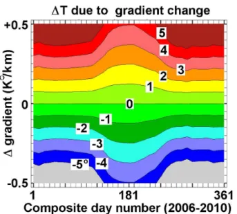
The empirical gradient used in SKiYMET processing is from Hocking et al. (2004). It can be seen in Eq. (5) that the gra-dient, usually of the order of several K km−1, is a secondary modifier to the temperature in comparison with themag/ k term (34.09), but it is a significant contributor to variations. Figure 1 shows the sensitivity of real temperature results to small changes in the empirical 90 km gradients. A simple rule of thumb we will use hereafter is that the temperature result change is approximately 10 times the gradient change, and in
Fig. 1.Sensitivity of SKiYMET temperatures to change in empiri-cal temperature gradient.
the same sense – that is, an increase in the assumed gradient leads to an increase in the temperature result.
Table 1.Comparison log10τ1/2slope estimates. MR are from fits to average and SD over all selected meteors at each height and month, 86–94 km. MR(MLS) is the same, but only those meteors for which MLS data are available are used (that is, where echo heights do not
come from one level beyond 0.001 mb); MLS are fits toτ1/2values from average dailyT,P (second-order polynomial fit to height profile)
and inversion of Eq. (6) for each meteor height. The SKiYMET slope was found by inverting Eq. (4) (with a priori knowledge of the daily temperature output and the temperature gradient model that was used). The latter involved very careful detailed meteor echo selection criteria and a specialized fit (Hocking et al., 1997). All results are for composite year: February 2006–June 2012.
−dlog10τ1/2/dz(km−1), 86–94 km except 86–91 km*
Month MR MR (MLS) MLS SKiYMET
Jan 0.041±0.031 0.041±0.031 0.064±0.008 0.066±0.004
Jul 0.055±0.034 0.048±0.067* 0.132±0.013* 0.108±0.008
The data marked “*” are for the height layer 86–91 km only.
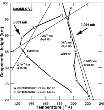
Fig. 2.Illustration of the3 pt. fitand9 pt. fitgradient calculation methods on MLS winter and summer temperature profiles.
the 34.09 in Eq. (5), their exact choice is not critical to MR-derived temperature results.
In the summer the model gradient is+0.6 K km−1, while the average MLS value is∼4 K km−1. If the3 pt. fitmethod is used, the gradient difference is much reduced, with MLS summer values around+2 K km−1. An argument for this gra-dient is that, given the MLS height resolution of ∼14 km near 90 km, the 3 heights almost cover the whole meteor layer. An argument for the9 pt. fitis that the linear fit may produce a more stable value.
It will be seen later that replacing the empirical gradi-ent value with these satellite gradigradi-ents according to Eq. (5) can drastically increase an already existing summer differ-ence between the two temperature measurements. Possible
Fig. 3. Comparison between the SKiYMET empirical gradient
model and the9 pt. fitMLS gradients.
reasons for this summer discrepancy include non-ambipolar trail dispersion, and will be discussed later.
Fig. 4.Illustration of the potential additive temperature perturbation (green trace) if the empirical gradient model were replaced, as in Eq. (5) by MLS day-to-day gradients (see text).
improved? There are at least two satellite passes per day within∼230 km of Eureka. (At this latitude MLS passes are spaced by∼460 km.)
Figure 4 shows a 2007/2008 winter-centred comparison between the original “online” SKiYMET temperatures and the proposed additive modification generated by MLS gra-dients. We take this opportunity to also show MLS versus MR temperature (but the main comparison will be based on the year 2008/2009 to be shown in Sect. 5.) The bot-tom (green) trace shows the expected day-to-day tempera-ture variation which would be produced by use of the day-to-day MLS temperature gradient variations, according to
1T =10(G2−G1)/2, whereG1andG2are the MLS gra-dients on adjacent days, and the factor of 10 comes from dis-cussion of Fig. 1. Its scale is the same as for temperature but the offset is arbitrary. The direct temperature agreement is not very good to begin with in this particular winter. How-ever it is clear that adding the day-to-day MLS gradient vari-ation term would make the agreement worse. So the use of a longer term, smooth, gradient model seems justified, and may better match reality.
4 The pressure method
An alternate analysis (e.g. Holdsworth et al., 2004; Dyrland et al., 2010), here called thepressure method, relies on know-ing a value forK0and on the availability of pressure data at 90 km.
Equation (1) can be usefully re-arranged as
T =
s
CP τ1/2
, (6)
where
C= qe
2k· T0
P0· ln 2λ2
16π2K 0
. (7)
Fig. 5.Winter-centred 5 day average log10P (mb) at 90 km (GPH)
and latitude 79.9◦N, longitude 86◦±13◦W: individual years and
7-year composite mean.
Fig. 6.Illustration of the pressure method: histograms of individual
trail temperatures,T, over a month: separate hours and combined
(“all”). On each trace the right ticks indicate medianTs the left,
averageTs.
could be to take medians over 5 day intervals for the speci-fied years, while if theP variations are real, then daily val-ues are even more appropriate. An obvious qval-uestion regard-ing use of MLS pressure data is this: if we have MLS GPH (used to get pressure at 90 km) then we probably also have MLS temperatures, so why do we need the radar? Our an-swer is that we want to check the use of empirical gradient and pressure models for effectiveness in times when satellite data are not available. Also, if the comparison is found suit-able, and diurnal variations in gradient and pressure are suffi-ciently low, we can get diurnal effects (i.e. tides) from meteor echoes without extra assumptions, as employed by Hocking and Hocking (2002), on the relation between wind and tem-perature tides (that is, that the vertical wavelengths are the same). Yuan et al. (2006) in a mid-latitude lidar study show
temperature and wind tidal data with sometimes major dif-ferences in vertical wavelength. Given that, in theory, we can get a usable temperature from each meteor with the input of daily average pressure, and from those get composite hourly temperature, whereas we need a large number of meteors and the assumption that the temperature gradient is constant over weeks or months to get an estimate ofS, the pressure method seems a more straightforward way to do tidal analysis. Fig-ure 6 shows this latter process: averages and medians from composite hourly histograms over a month are marked with tics. The pressure is from MLS 90 km daily average log10P near Eureka. There is a small expected average versus me-dian difference, but averages are easier to calculate, so we use that. Of course, a significant tidal signal in pressure may create insurmountable problems – that is, amplitude and/or phase shifts. This possibility is discussed further in Sect. 6.
In a way similar to Fig. 4 we have looked at daily changes in MLS pressure over 2007/2008 to see the effect on tem-perature results of using the same-day pressure whenτ1/2is assumed constant. The temperature change, by differentiat-ing Eq. (6), is given from1T /T =121P /P, where1T and
1P are the day-to-day daily differences at 90 km from MLS data, andT andP are the average temperature and pressure over each pair of days. The results (not shown) are thatT
“noise” of the order of±5 K or less is generated. This is of similar size to that generated by the use of day-to-day MLS temperature gradients shown in Fig. 4.
5 Direct comparisons between temperatures from MLS and the Eureka MR
Fig. 7. Comparison between 90 km temperatures calculated by the gradient method (upper panel, empirical model) and pressure method (lower panel, Aura MLS) for winter-centred 2008/2009. Be-low each comparison is a plot of the temperature differences: MLS minus Eureka MR.
6 Measured decay times compared with MLS-predicted times
6.1 Artificialτ1/2generated from MLST,P
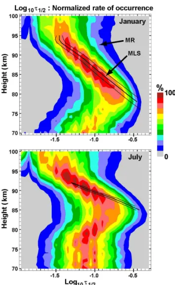
Since MLS provides pressure and temperature information, we can use Eq. (6) to calculate an appropriate τ1/2 value. The monthly relative occurrence of accepted meteor values (log10τ1/2) with (radar) height for six years (excepting some large winter intervals rejected due to excessive external noise from a co-located star photometer) for January and July are shown in Fig. 8. Although meteor echo occurrence is much reduced below∼80 km, this multi-year interval provides a good statistical sample. (The discrete nature of radar range measurements, 2 km steps, is responsible for the “pulses” in the contour.) Similar data presentations appear in Ballinger et al. (2008) for a year’s observations (all data combined) from the SKiYMET at Esrange, Sweden; Hall et al. (2005) combined January to June, while Kim et al. (2010) showed Antarctic data for 4 separate seasons.
Fig. 8.log10τ1/2calculated from Aura MLST andP by Eq. (6) compared with the Eureka MR percentage occurrence (relative to the total at each height over the 34 bins) in meteor trails for January and July (composite year 2006–2011 and part of 2012).
The equivalent MLS log10τ1/2has been calculated as fol-lows: GPH-T profiles for each day were interpolated to get average daily log10P and T from 70 to 100 km in steps of 1 km. The appropriate daily average profiles were inter-polated to the height of each meteor echo, and the corre-sponding MLS log10τ1/2found from Eq. (6). The monthly means and the one-standard-deviation limits of this parame-ter, which represent the assumption that ambipolar diffusion is the only dispersing effect (and also, of course, that MLS
Fig. 9.Composite year, monthly mean difference between measured
and MLS log10τ1/2. This is effectively log10(MLSDa/MRDa).
showing that dispersion is much stronger than ambipolar in the latter season.
Note that despite the visual agreement near 90 km, the pressure method value is very sensitive to log10τ1/2. For ex-ample, a change of 0.04 on this scale, at T =150 K, can change the temperature result by 30 K, so this apparent agree-ment at 90 km does not directly contradict the summer T
differences seen in Figs. 4 and 7. Also, from Eq. (6), tem-perature varies as
q
τ1/2−1, not log10τ1/2, so statistics of the latter parameter in Fig. 8 will produce somewhat dif-ferent temperature than shown in Figs. 4 or 7. The ma-jor winter/summer difference between MR and MLS data is the slope,dlog10τ1/2/dh. This will impact the gradient method. A similar comparison between winter τ1/2 from the SKiYMET system in Thumba, India, and that calcu-lated from the TIMED-SABER data archive for temperature and pressure was reported by Kumar and Subrahmanyam (2012). Their Fig. 2 for 88 km showsτ1/2-SABER∼0.135 and SKiYMET,∼0.10 s, If the data of Fig. 8 are reprocessed to obtain means ofτ1/2rather than log10τ1/2, the 88 km value in January for MLS is 0.084 s and for the Eureka SKiYMET, 0.095 s (both composite year 2006–2012). This may indicate a greater dispersion rate near the equator, or a difference inτ
statistics.
6.2 MLS log-decay time slopes versus various meteor options
It can be seen from Fig. 8 that the slope of log10τ1/2, i.e.S in Eq. (3), in summer is apparently less than would be pre-dicted by MLS assuming only ambipolar diffusion. There-fore temperatures calculated by the gradient method, which are inversely proportional toS, would be biased high. If MLS temperatures are considered to be appropriate, this can
ex-plain at least part of the MR–MLS temperature difference in Figs. 4 and 7. Four types of log10τ1/2slope estimates,S, are listed in Table 1 for January and July of the composite year February 2006–June 2012.
Those labelled “MR” are from fits to average and SD over all selected meteors at each height and month, 86–94 km. “MR(MLS)” are the same, but only those meteors for which MLS data are available are used (that is, where echo heights do not come from one level beyond 0.001 mb), “MLS” indi-cates fits toτ1/2values from average dailyT andP (second-order polynomial fit to height profile) and inversion of Eq. (6) for each meteor height. The SKiYMET slope was found by inverting Eq. (4) (with a priori knowledge of the daily tem-perature output and the temtem-perature gradient model that was used). The latter involved very careful and detailed meteor echo selection criteria and a specialized fit (Hocking et al., 1997). All results are for composite year: February 2006– June 2012.
With regard to the January results in Table 1, the MLS “S” and SKiYMET “S” overlap within error, whereas the “MR” and “MR(MLS)” slopes are quite different and, since the fi-nal temperature depends on 1/S, would lead to a major differ-ence between MR and MLS. Thus careful selection of meteor echoes in the gradient method, as described in Hocking et al. (1997), is absolutely necessary.
The fact that the local MLS “S” also decreases above 94 km probably says something about the accuracy of MLS
T at these these non-recommended heights, and if so, has made the MLS-fitted “S” value somewhat less than it actu-ally should be around 90 km. But the table values and vi-sual appearance suggest the distortion is minor. The tabled July results show very large discrepancies between the var-ious slopes. Careful meteor selection (“SKiYMET”) results in an S closer to the “MLS value”, but there is still about 20 % difference; that is, SKiYMET temperatures could be 20 % greater than those from MLS. At (summer) tempera-tures of∼130 K, that amounts to 26 K, a difference which is similar to that seen. If a smaller summer temperature gra-dient had been used in the analysis, the temperature discrep-ancy would be reduced. However, that would leave a larger disparity between the empirical model and MLS gradients. Also, the model gradient would actually have to be slightly negative to get good agreement.
Fig. 10.Monthly (composite year, 2006–2012) diurnal temperature (T (pressure method), and northward (V) and eastward (U) wind varia-tions at 90 km. The 24 h mean has been subtracted from each monthly “day”.
the mid-signal range in all months, and except for extremely high and low S/N bins the variation in any month was within one standard deviation. A similar result was found when just two morning hours were selected, and also for 82.0–84.0 km. We do not see the predicted relation between echo strength andτ1/2, but that does not rule out the possibility that dust affects decay times.
6.3 A possible explanation for the MLS-MR log-decay time slope difference
We show in Fig. 9 the monthly average difference between MLS and MR log10τ1/2 data from Fig. 8. SinceDa is in-versely proportional to√τ1/2, the value plotted is, in effect, the log of the ratio ofDaestimates, in the sense MLS/MR.
Meteor echo spatial scales are similar to those sampled by rockets, so these are a good choice for a first compari-son. L¨ubken (1997), in a study of winter and summer arctic turbulence measurements from multiple rocket statistics of neutral density fluctuations, showed that summer turbulent diffusion coefficients from∼85 to 90 km were significantly larger than those in winter (his Fig. 11). Hall et al. (1999) showed seasonal detail from rocket results (their Fig. 2) with a similar winter/summer difference, though the early summer is not well represented in their available data. And finally Kim et al. (2010) show a summer/winter difference similar to Fig. 8 with Antarctic meteor data in both weak and strong trails (their Fig. 2). So it appears that turbulence, at least on rocket scales, is a likely contributor to the MR/MLS summer temperature disagreement. Further discussion on this matter will be left for a future paper.
7 Estimation of temperature tides
Figure 10 contains contour plots of (composite year 2006– 2012 partial) diurnal variations for each month of temper-ature (89.0–91.0 km, by pressure method), and horizontal wind (91 km, from fit to meteor echo location and radial ve-locities,Vr, in 3 km layers, with additional selection criteria: zenith 10–70◦, and relative error inVr<25 %). Although we call the MLS pressure a daily pressure, MLS samples only twice a day at two almost constant times, 10:00–11:00 and 15:00–16:00 UTC (ascending and descending nodes), The times are not exact, because the longitude of the nearest pass varies, but for Eureka their difference is always close to 6 h in local time, and, more importantly, those two samples are always at the same two phases of any seasonally constant mi-grating tide. For example, if the first sample is of a zero of the semi-diurnal tide, the second will always be of a zero, if it is of a maximum, the second will be of a minimum, etc.
The problem is that a constantP during the day is applied to get temperature fromτ1/2, so any diurnalPvariations rep-resent a hidden perturbation which should be added to this temperature result. If theP variations are large enough, they could lead to significant errors in the estimated tide ampli-tudes and/or phases. Thus we want to know what pressure variations to expect.
Another is the Canadian Middle Atmosphere Model with data assimilation, CMAM-DAS (Ren et al., 2008), which has hourly data up to 88 km. log10P (mb) is found to have diur-nal peak-to-peak variations of about 0.02 in winter and 0.03 in summer (but the 24 and 12 h components for the monthly mean day are not clearly visible). We could also get MLS
∼6 h local-time pressure difference statistics at 80◦N by av-eraging the differences of all single-orbit ascending (A) and descending (D) node pressures (to eliminate longitude vari-ations), but since the two sample times are fixed relative to the tide, the measurement would only represent the minimum possible pressure variation, whereas we would like the maxi-mum. Despite this limitation, and for completeness, we have calculated the root mean square of the 91 km, 79.7◦N, rela-tive pressure difference,(PA−PD)/(PA+PD), to be∼1 % in all months (rising to∼5 % at 80.7◦N). Since temperature varies as the square root of pressure (Eq. 6), this represents a temperature fluctuation of about 0.5 % (2.5 % at 80.7◦N), which is small compared to the maximum diurnal variation of∼ ±6 K seen in Fig. 10. However the variance of a dif-ference includes the variance of each sample, i.e. MLS mea-surement errors, so the actual pressure difference should be somewhat smaller. Despite these arguments we cannot ignore the possibility that the data shown are contaminated because of unaccounted diurnal pressure variations.
8 Conclusions
1. We cannot resolve the summer discrepancy between the empirical gradient model and MLS gradients (Fig. 3). A better agreement is found with local 90 km MLS gradi-ents, but it is somewhat unreasonable to use this single height estimate with a thick meteor layer, especially in summer, when there is strong temperature variation with height. On the other hand, since the log10τ1/2gradient is expected to be effectively weighted by the peak meteor rate around 90 km, employment of aT gradient some-where between the local and the 9 km layer fit seems more reasonable given that the echoes are from thick layer. But the discrepancy inT gradient, though smaller, remains. Since the gradients used here are from sim-ple fits which ignore height resolution and temperature precision, and not a MLS product, we cannot choose a definitive value.
2. For winter both the temperature gradient (using the em-pirical model) and the pressure method (using interpo-lated 90 km MLS 5 day pressures) daily meteor temper-atures agree quite well with MLS data in short, several day, fluctuations, and the Kelvin temperatures are also in good agreement (Fig. 7).
3. But in summer, at least to 2006–2009, good agreement is found in temperatures between pressure and temper-ature gradient methods but not with MLS. Both MR
log10τ1/2and its height gradient would have to be big-ger to match the summer MLS values (given the same temperature gradient model and the physical constants used in the pressure method). Use of MLS gradients in place of the model increases the disagreement.
Although this present work does not discuss data be-yond 2009, we have noted that for the summers of 2010, 2011, 2012, the gradient method temperature is lower by∼10◦than in previous years, which puts it in bet-ter agreement with MLS, while the MLS value does not change significantly summer to summer over this 7-year period. In order for this change to occur, the SKiYMET
Smust have changed for these recent summers without a significant modification of log10τ1/2near 90 km (be-cause the pressure method value did not change). This feature remains under investigation.
Temperature fluctuations in summer are small, so short-term agreement is hard to assess.
4. Regarding the tidal analysis, available model diurnal pressure variations (CMAM-DAS and MSISE-00) and such estimates as are available from MLS have shown that use of a fixed daily pressure may lead to significant distortion of temperature tide results.
5. Comparisons of directly measured meteor echo decay times, τ1/2, through the mesosphere (75–95 km) with estimates ofτ1/2, based solely upon MLS data and the assumed dominance of ambipolar diffusion, show large differences near and below 90 km, especially in summer months. This is consistent with the competitive effects of neutral turbulence. Detailed assessments of seasonal variations of eddy or turbulent diffusion from meteor and medium frequency radar soundings are proposed to bolster the limited rocket data available: these latter suggest larger turbulence in the summer’s mesopause region.
Acknowledgements. The authors are grateful to the Jet Propulsion Lab (JPL) for access to the Aura MLS data. We appreciate the help of Michael Neish (University of Toronto) in providing access to the CMAM-DAS 1 h data, and thank the Institute of Space and At-mospheric studies, through the University of Saskatchewan, for re-search facilities, and Canada’s National Sciences and Engineering Research Council (NSERC) for financial support through a Discov-ery Grant. Finally, we appreciate the careful assessment and sug-gestions by the two reviewers.
Topical Editor C. Jacobi thanks G. Stober and one anonymous referee for their help in evaluating this paper.
References
the polar mesopause region, Ann. Geophys., 26, 3439–3443, doi:10.5194/angeo-26-3439-2008, 2008.
Das, S. S., Kumar, K. K., Das, S. K., Vineeth, C., Pant, T. K., and Ramkumar, G.: Variability of mesopause temperature de-rived from two independent methods using meteor radar and its comparison with SABER and EOS MLS and a co-located multi-wavelength dayglow photometer over an equatorial station, Thumba (8.5 N, 76.5 E), Int. J. Remote Sens., 33, 4634–4647, 2012.
Dyrland, M, E., Hall, C. M., Mulligan, F. J., Tsutsumi, M., and Sigernes, F.: Improved estimates for neutral air temperatures at 90 km and 78 N using satellite and meteor radar data, Radio Sci., 45, RS4006, doi:10.1029/2009RS004344, 2010.
Dyrud, L. P., Urbina, J., Fentzke, J. T., Hibbit, E., and Hinrichs, J.: Global variation of meteor trail plasma turbulence, Ann. Geo-phys., 29, 2277–2286, doi:10.5194/angeo-29-2277-2011, 2011. Hall, C. M.: On the influence of neutral turbulence on ambipolar
dif-fusivities deduced from meteor trail expansion, Ann. Geophys., 20, 1857–1862, doi:10.5194/angeo-20-1857-2002, 2002. Hall, C. M., Hoppe, U. P., Blix, T. A., Thrane, E. V., Manson, A.
H., and Meek, C. E.: Seasonal variation of turbulent energy dis-sipation rates in the polar mesosphere: a comparison of methods, Earth, Planets, and Space, 51, 515–524, 1999.
Hall, C. M., Aso, T., Tsutsumi, M., Nozawa, S., Manson, A. H., and Meek, C. E.: Letter to the Editor: Testing the hypothesis of the influence of neutral turbulence on the deduction of ambipo-lar diffusivities from meteor trail expansion, Ann. Geophys., 23, 1071–1073, doi:10.5194/angeo-23-1071-2005, 2005.
Havnes, O. and Sigernes, F.: On the influence of background dust on radar scattering from meteor trails, J. Atmos. Sol.-Terr. Phys., 67, 659–664, 2005.
Hocking, W. K.: Temperatures using radar-meteor decay times, Geophys. Res. Lett., 26, 3297–3300, 1999.
Hocking, W. K.: Experimental radar studies of anisotropic diffusion of high altitude meteor trails, Earth, Moon, and Planets, 95, 671– 679, doi:10.1007/s/11038-005-3446-5, 2004.
Hocking, W. K. and Hocking, A.: Temperature tides deter-mined with meteor radar, Ann. Geophys., 20, 1447–1467, doi:10.5194/angeo-20-1447-2002, 2002.
Hocking, W. K., Thayaparan, T., and Jones, J.: Meteor decay times and their use in determining a diagnostic mesospheric temperature-pressure parameter methodology and one year of data, Geophys. Res. Lett., 24, 2977–2980, 1997.
Hocking, W. K., Singer, W., Bremer, J., Mitchell, N. J., Batista, P., Clemshea, B., and Donner, M.: Meteor radar temperatures at multiple sites derived with SKiYMET radars and compared to OH, rocket, and lidar measurments, J. Atmos. Sol.-Terr. Phys., 66, 585–593, 2004.
Holdsworth, D. A., Reid, I. M., and Cervera, M. A.: Buckland Park all-sky interferometric radar, Radio Sci., 39, RS5009, doi:10.1029/2003RS003014, 2004.
Kim, J.-H., Kim, Y. H., Lee, C.-S., and Jee, G.: Seasonal variation of meteor decay times observed at King Sejong Station (62.22 S, 58.78 W), Antarctica, J. Atmos. Sol.-Terr. Phys., 72, 883–889, 2010.
Kumar, K. K.: Temperature profiles in the MLT
re-gion using radar-meteor decay times: Comparison with TIMED/SABER observations, Geophys. Res. Lett., 34, L16811, doi:10.1029/2007GL030704, 2007.
Kumar, K. K. and Subrahmanyam, K. V.: A discussion on the as-sumption of ambipolar diffusion of meteor trails in the Earth’s upper atmosphere, Monthly Not. R. Astron. Soc. Lett., 425/1, doi:10.1111/j.1365-2966.2012.20504.x, 2012.
L¨ubken, F.-J.: Seasonal variation of turbulent energy dissipation rates at high latitudes as determined by in situ measurements of neutral density fluctuations, J. Geophys. Res., 102, 13441– 13456, 1997.
Manson, A. H., Meek, C. E., Chshyolkova, T., Xu, X., Aso, T., Drummond, J. R., Hall, C. M., Hocking, W. K., Jacobi, Ch., Tsut-sumi, M., and Ward, W. E.: Arctic tidal characteristics at Eureka
(80◦N, 86◦W) and Svalbard (78◦N, 16◦E) for 2006/07:
sea-sonal and longitudinal variations, migrating and non-migrating tides, Ann. Geophys., 27, 1153–1173, doi:10.5194/angeo-27-1153-2009, 2009.
Manson, A. H., Meek, C. E., Xu, X., Aso, T., Drummond, J. R., Hall, C. M., Hocking, W. K., Tsutsumi, M., and Ward, W. E.: Characteristics of Arctic winds at CANDAC-PEARL
(80◦N, 86◦W) and Svalbard (78◦N, 16◦E) for 2006–2009:
radar observations and comparisons with the model CMAM-DAS, Ann. Geophys., 29, 1927–1938, doi:10.5194/angeo-29-1927-2011, 2011.
Picone, J. M., Hedin, A. E., Drob, D. P., and Aikin, A. C.: NRLMSISE-00 empirical model of the atmosphere: Statistical comparisons and scientific issues, J. Geophys. Res., 107, 1468, doi:10.1029/2002JA009430, 2002.
Ren, S., Polavarapu, S. M. and Shepherd, T. G.: Vertical propagation information in a middle atmosphere data assimilation system by gravity-wave drag feedbacks, Geophys. Res. Lett., 35, L06804, doi:10.1029/2007GL032699, 2008.
Schwartz, M. J., Lambert, A., Manney, G. L., Read, W. G., Livesey, N. J., Froidevaux, L., Ao, C. O., Bernath, P. F., Boone, C. D., Cofield, R. E., Daffer, W. H., Drouin, B. J., Fetzer, E. J., Fuller, R. A., Jarnot, R. F., Jiang, J. H., Jiang, Y. B., Knosp, B. W., Kr¨uger, K., Li, J.-L. F., Mlynczak, M. G., Pawson, S., Russell III, J. M., Santee, M. L., Snyder, W. V., Stek, P. C., Thurstans, R. P., Tomp-kins, A. M., Wagner, P. A., Walker, K. A., Waters, J. W., and Wu, D. L.: Validation of the Aura Microwave Limb Sounder temper-ature and geopotential height measurements, J. Geophys. Res., 113, D15S11, doi:10.1029/2007JD008783, 2009.
Stober, G., Jacobi, C., Matthias, V., Hoffmann, P., and Gerding, M.: Neutral air density variations during strong planetary wave activ-ity in the mesopause region derived from meteor radar observa-tions, J. Atmos. Sol.-Terr. Phys., 74, 55–63, 2012.
Yuan, R., She, Y., Hagan, M. E., Williams, B. P., Li, T., Arnold, K., Kawahara, T. D., Acott, P. E., Vance, J. D., Kreuger, D., and Roble, R. G.: Seasonal variations in mesopause region temperature, zonal and meridional winds above Fort Collins,
Colorado (40,6◦N, 105◦W), J. Geophys. Res., 111, D06103,