Comput. Appl. Math. vol.25 número23

(1)

ISSN 0101-8205 www.scielo.br/cam

A unified regularization theory: the maximum

non-extensive entropy principle

HAROLDO F. DE CAMPOS VELHO1_{, ELCIO H. SHIGUEMORI}2

FERNANDO M. RAMOS1 and JOÃO C. CARVALHO3

1_{Instituto Nacional de Pesquisas Espaciais (INPE)}

Laboratório Associado de Computação e Matemática Aplicada (LAC) São José dos Campos, SP, Brazil

2_{Instituto de Estudos Avançados (IEAv)}

Comando Geral Brasileiro de Tecnologia Aeroespacial (CTA) São José dos Campos, SP, Brazil

3_{Agência Nacional de Telecomunicaç˜eos (ANATEL)} Brasília, DF, Brazil

E-mails: [haroldo, elcio, fernando]@lac.inpe.br / [email protected]

Abstract. Tsallis’ non-extensive entropy is used as a regularization operator. The parameter

“q” (non-extensivity parameter) has a central role in the Tsallis’ thermostatiscs formalism. Here, several values ofqare investigated in inverse problems, usingq <1 andq>1. Two standard regularization techniques are recovered for specialq-values: (i)q=2 is the well known Tikhonov regularization; (ii)q=1 is the standard Boltzmann-Gibbs-Shannon formulation for entropy. The regularization feature is illustrated in an inverse test problem: the estimation of initial condition in heat conduction problem. Two methods are studied for determining the regularization parameter, the maximum curvature for theL-curve, and the Morozov’s discrepancy principle. The new regularization of higher order is applied to the retrieval of the atmospheric vertical profile from satellite data.

Mathematical subject classification: 35R30.

Key words: Maximum non-extensive entropy pinciple, unified regularization theory, inverse

problems.

(2)

1 Introduction

Inverse problems belong the class ofill-posed problems. In these type of

prob-lems existence, uniqueness and stability of their solutions cannot be ensured. The regularization theory appeared in the 60’s as a general method for solv-ing inverse problems [1]. In this approach, the non-linear least square prob-lem is associated with a regularization term (a priori or additional

informa-tion), in order to obtain a well-posed problem. A well-known regularization technique was proposed by Tikhonov [1], where smoothness of the unknown function is searched. Similarly to Tikhonov’s regularization, the maximum en-tropy formalism searchs forglobal regularity and yields the smoothest recon-structions which are consistent with the available data. The maximum entropy principle was first proposed as a general inference procedure by Jaynes [2] on the basis of Shannon’s axiomatic characterization of the amount of informa-tion [3]. This principle has successfully been applied to a variety of fields. In the middles of 90’s, higher order procedures for entropic regularization have been introduced [5, 6] (see also [7] and references inside).

In the macrocospic thermodynamics, the entropy is applied to quantify the irreversibility in systems, and the entropy has a fundamental role in the statistical physics. The Shannon’s entropy is a measurement of the missing information. In the inverse problem context, it is ashape entropy.

A non-extensive formulation for the entropy has been proposed by Tsallis [8, 9]. Recently, the non-extensive entropic form (Sq) was used as a new regularization

operator [10], using only q = 0.5. The q parameter plays a central role in

the Tsallis’ thermostatistics, in whichq = 1 the Boltzmann-Gibbs-Shannon’s entropy is recovered. As mentioned, the non-extensive entropy includes as a particular case the extensive entropy (q = 1): in which the maximum entropy principle can be used as a regularization method. However, another important particular case of the non-extensive entropy occurs whenq =2. In such case, the maximumnon-extensiveentropy principle to theS2regularization operator

is equivalent to the standard Tikhonov regularization (or zeroth-order Tikhonov regularization) [1, 11].

(3)

q were used for thenon-extensiveentropic regularization term. Synthetic data

with Gaussian white noise corruption were used to simulate experimental data. Two methods were investigated for determining the regularization parameter: the Morozov’s discrepancy principle [13], and the maximum curvature scheme of the curve relating smoothness versus fidelity, inspired in Hansen’s geometrical criterion [14].

Initial conditions for numerical weather prediction are obtained from the Earth observation system. Radiances measured by meteorological satellites is a com-ponent of this observation system. From these radiances, atmospheric tem-perature and humididy profiles can be determined. Several methodologies and models have been developed to compute this estimation. A method using the second order entropy approach [7] was proposed as a solution for this inverse problem. Here, the higher order non-extensive entropy will be used to improve the previous inverse solution.

Non-extensive entropy as a new regularization operator

A non-extensive form of entropy has been proposed by Tsallis [8] by the expres-sion

Sq(p)=

k

q−1



1−

Np

X

i=1

pq_i



 (1)

where pi is a probability, and q is a free parameter. In thermodynamics the

parameterk is known as the Boltzmann’s constant. Similarly as in the

mathe-matical theory of information,k =1 is considered in the regularization theory. Tsallis’ entropy reduces to the the usual Boltzmann-Gibbs-Shanon formula

Sq(p)= −k

Np

X

i=1

pi lnpi (2)

in the limitq →1.

As for extensive form of entropy, the equiprobability condition produces the maximum for the non-extensive entropy function, and this condition is ex-pressed as

Sq

max=

1 1−q N

1−q

p −1

(4)

where, in the limitNp→ ∞,Sqdiverges ifq ≤1, and saturates at 1/(q−1)if

q >1 [9].

The equiprobability condition leads the regularization function defined by the operatorSq(p), given by Eq. (1), to search the smoothest solution for the of the

unknown vectorp.

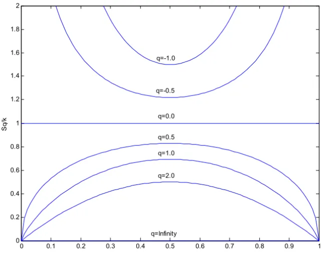
The parameterq has a central role in Tsallis’ thermostatiscs, and it is called

thenon-extensivity parameter– see Eqs. (A.5) and (A.6) in the Appendix.

Fig-ure 1 shows the functional form for the Tsallis’ entropy for several values ofq.

Forq < 5/3, the standard central limit theorem applies, implying that if pi is

written as a sum ofMrandom independent variables, in the limit caseM→ ∞, the probability density function for pi in the distribution space is thenormal

(Gaussian) distribution [9]. However, for 5/3 < q < 3 the Levy-Gnedenko’s central limit theorem applies, resulting forM → ∞the Levy distribution as the

probability density function for the random variablepi. The index in such Levy

distribution isγ =(3−q)/(q−1)[9].

0 0.1 0.2 0.3 0.4 0.5 0.6 0.7 0.8 0.9 1 0

0.2 0.4 0.6 0.8 1 1.2 1.4 1.6 1.8 2

p

S

q

/k

q=-1.0

q=-0.5

q=0.0

q=0.5 q=1.0

q=2.0

q=Infinity

(5)

The non-extensive approach has been used in many different applications, such as in a certain type of anomalous diffusion process [9], as well as the statistical model for data from turbulent flow [15] and from financial market [16]. Accord-ing to Plastino and Plastino [17], the first experimental confirmation of Tsallis’ non-extensive formalism is the Boghosian’s approach of the two dimensional pure electron plasma [18]. Some properties of the thermostatistics formalism are described in the Appendix.

Regularization unified

Some comments have been addressed for indicating the physical properties of theSqoperator. The goal of this Section is to describe formally the properties for

this operator looking at regularization purposes. Regularization properties for entropy operator emerges from the Jaynes’ inference criterium: the maximum entropy principle, where all events have the same propability to occur. Implying that all parameters assume the same value: pi =1/Np. The following Lemma

extends this result for non-extensive entropy.

Lemma. The non-extensive function Sqis maximum as pi =1/Npfor all i.

Proof. The problem is to find the maximum of the function (1), with the

fol-lowing constrain

Np

X

i=1

pi =1 (4)

sincepi represents a probability. Therefore, it is possible to define an objective

function where the constrain can be added to the non-extensive function:

J(p)=Sq(p)+λ





Np

X

i=1

pi−1



 (5)

whereλis the Langrange multiplier. The Lagrange multiplier, in this case, can be determined when a minimum for the objective function J(p) is found, as following

∂J

∂pi

= −q p_iq−1+λ(q−1)=0 ⇒ pi =

λ(q−1)

q

_q₋1₁

(6)

This result can be used to obtain the value of thepi’s that maximizes the function

J(p):

Np

X

i=1

pi =

Np

X

i=1

λ(q−1)

q

_q₋1₁

=

λ(q−1)

q

_q1₋₁

Np=1 ⇒ pi =

1

Np

(7)

that means ifpi =1/Npfor alli =1, ...,Npthe non-extensive entropy function

is maximum.

The next theorem shows that the extensive entropy and Thikhonov’s regular-izations are particular cases of the non-extensive entropy.

Theorem. For particular values for non-extensive entropy q =1and q =2

are equivalents to the extensive entropy and Tikhonov regularizations, respec-tively.

Proof. (i) q =1: Taking the limit,

lim

q→1Sq(p) = qlim→1

1−PNp i=1p

q i

q−1 =qlim→1

1−PNp i=1eqlogpi

q−1

= lim

q→1

−PNp

i=1logpieqlogpi

1 = −

Np

X

i=1

pilogpi

(8)

(ii) q =2: Remembering that maxS2is equivalent to min(−S2), yields

maxS2(p) = max



1−

Np

X

i=1

p_i2



 ⇔ min [−S2(p)]

= min





Np

X

i=1

p_i2−1





(9)

now, for the maximum (minimum) value holds∇_pS2=0, therefore

∇pS2(p)= ∇p





Np

X

i=1

p2_i −1



= ∇p





Np

X

i=1

p_i2



= ∇pkpk2₂ (10)

In conclusion: maxS2(p) = minkpk22 (the zeroth-order Tikhonov

(7)

Inverse analysis

Typically, inverse problems are ill-posed – existence, uniqueness and stability of their solutions cannot be ensured. An inverse solution can be formulated to obtain existence and uniqueness, but this solution can still be unstable under the presence of noise in the experimental data. Hence, it requires some regu-larization technique, i.e., the incorporation in the inversion procedure of some available information about the true solution. Following the Tikhonov’s ap-proach [1], a regularized solution is obtained by choosing the function p∗ that

minimizes the following functional

Jα[ ˜8,p] =

˜

8−8(p)

2

2+α [p] (11)

where₈˜ _{is the experimental data,} ₈₍_p₎_{is the answer computed from the}

for-ward model, [p] denotes the regularization operator, α is the regularization parameter, andk∙k2is theL2norm.

The regularization parameter α is chosen by two methods: numerically, as-suming that a boundδ (or the ‘statistics’) of the measurement error is known, i.e.,

8computed− ˜8

≤ δ — this numerical procedure is based on Morozov’s

discrepancy principle [13]; graphically, finding out the point of maximum cur-vature in the curve[pα] ×

˜

8−8(pα)

2

2, a type of L-curve [14, 19].

Optimization algorithm

The optimization problem is iteratively solved by the quasi-newtonian optimizer routine from the NAG Fortran Library [20]. This algorithm is designed to min-imize an arbitrary smooth function subject to constraints (simple bound, linear or non-linear constraints), using a sequential programming method.

This routine has been successfully used in several previous works: in geo-physics, hydrologic optics, and meteorology.

Backward heat conduction

(8)

mathematical formulation of this problem is given by the following heat equation

∂2T(x,t)

∂x2 =

∂T(x,t)

∂t , x ∈(0,1), t>0, (12)

∂T(x,t)

∂x =0, x =0; x =1, t>0, (13)

T(x,t)= f(x), x ∈ [0,1], t =0, (14)

where T(x,t)(temperature), f(x) (initial condition), x (spatial variable) and t(time variable) are dimensionless quantities. The set of partial differential

equa-tions is solved by using a central finite difference approximation for space vari-ableO(1x2), and explit Euler method for numerical time integrationO(1t)[21]. This problem has been used for testing different methodologies in inverse problems [12, 11, 22, 23, 24], and it is badly conditioned problem [12].

The numerical experiment with the non-extensive entropy is based on two test functions, the triangular function

f(x)=

(

2x, 0≤x <0.5, 2(1−x), 0.5≤ x ≤1;

(15)

and semi-triangular function

f(x)=



           

           

0.55, 0≤x <0.2,

8 3x+

7

15, 0.2≤x <0.5,

−28

5 x+ 23

5 , 0.5≤x <0.75, 2

9, 0.75≤x ≤1.

(16)

The experimental data (measured temperatures at a timet >0), which intrinsi-cally contains errors, is obtained by adding a random perturbation to the exact solution of the direct problem, such that

˜

(9)

whereσ is the standard deviation of the errors, andμis a random variable taken from a Gaussian distribution, with zero mean and unitary variance. All tests were carried out using 5% of noise (σ =0.05).

It is important to observe that the spatial grid consists of 101 points (Nx =101),

and the time-integration is performed up tot=0.01. The residueR(fα)and the errorE(fα)are defined by

R(fα) ≡

˜

T −T(fα)

2 2

; (18)

E(fα) ≡

fα− fexact

2 2

. (19)

If we effectively want to apply some kind of regularization, which meansα >0 in Eq. (5), then the discrepancy principle – ana-posterioriparameter choice rule – implies that a suitable regularized solution can be obtained. Since the spatial resolution isNx =101, the optimumαis reached forR(f∗)≃ Nxσ2 =0.2525.

Table 1 shows the square diference term R(f∗)obtained for different values of

α, and theoptimumvalue is pointed out for each case in bold font.

Triangular function Semi-triangular function

α R(fα) E(fα) α R(fα) E(fα)

0.0001 0.1853 2.7298 0.0001 0.1851 4.9359

0.0003 0.1856 0.5388 0.0003 0.1854 0.6740

0.0010 0.1861 0.3443 0.0010 0.1856 0.3443

0.0285 0.2525 0.3994 0.0346 0.2525 0.2400

0.0999 0.7728 0.8684 0.0999 0.6687 0.7207

Table 1 – Determining regularization parameter by Morozov’s criterion:q =0.5.

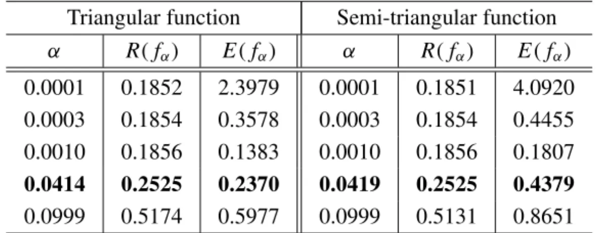
A set of tables (Tables 1 and 2) presents the least squares (or residual) term

R(fα) and the error E(fα) between the approximated (or calculated) solution

fα and the exact solution fexactobtained for two values ofq =0.5 andq =2.0,

from a family of regularization non-extensive entropy functionsSq, for different

(10)

α R(fα) E(fα) α R(fα) E(fα)

0.0001 0.1852 2.3979 0.0001 0.1851 4.0920

0.0003 0.1854 0.3578 0.0003 0.1854 0.4455

0.0010 0.1856 0.1383 0.0010 0.1856 0.1807

0.0414 0.2525 0.2370 0.0419 0.2525 0.4379

0.0999 0.5174 0.5977 0.0999 0.5131 0.8651

Table 2 – Determining regularization parameter by Morozov’s criterion:q =2.0.

10 20 30 40 50 60 70 80 90 100 0 0.1 0.2 0.3 0.4 0.5 0.6 0.7 0.8 0.9 1 x In it ia l T e m p e ra tu re

10 20 30 40 50 60 70 80 90 100 0 0.1 0.2 0.3 0.4 0.5 0.6 0.7 0.8 0.9 1 x In it ia l T e m p e ra tu re (a) (b)

10 20 30 40 50 60 70 80 90 100 0 0.1 0.2 0.3 0.4 0.5 0.6 0.7 0.8 0.9 1 x In it ia l T e m p e ra tu re (c) (d)

(11)

10 20 30 40 50 60 70 80 90 100 0 0.1 0.2 0.3 0.4 0.5 0.6 0.7 0.8 0.9 1 x In it ia l T e m p e ra tu re (a) (b)

10 20 30 40 50 60 70 80 90 100 0 0.1 0.2 0.3 0.4 0.5 0.6 0.7 0.8 0.9 1 x In it ia l T e m p e ra tu re (c) (d)

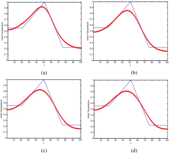
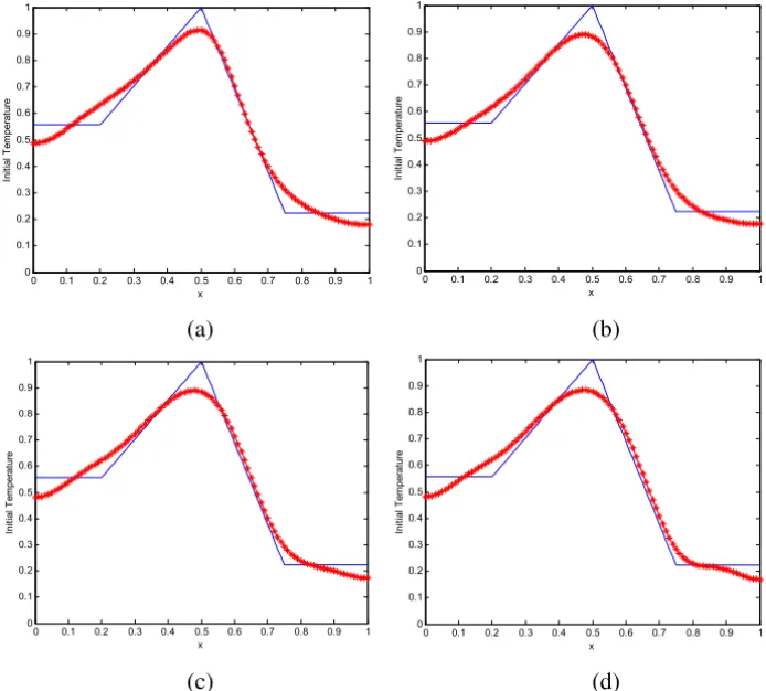
Figure 3 – Reconstructions with 5% of noise, with a determined by Morozov’s principle: (a)q =0.5; (b)q=1.5; (c)q =2.0; (d)q =2.5.

The parameter vector was always subjected to the following simple bounds: 1.2 ≥ fk ≥ −0.2 for the triangular test function, and 1.2 ≥ fk ≥ 0 for the

semi-triangular test function, withk =1,2, . . . ,Nx.

Figures 3a–3d show the estimation of fourq-values for triangular initial con-dition, where the regularization parameter was computed by Morozov’s princi-ple. The best reconstruction was found byq = 2.5, but good reconstructions were obtained for other values ofq too. Figures 2a–2d depict the reconstruc-tions for the semi-triangular test function, showing good reconstrucreconstruc-tions for all values of q.

(12)

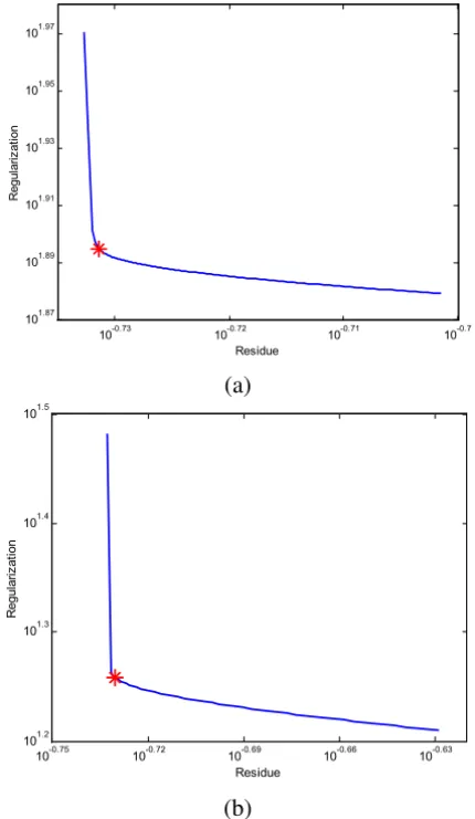
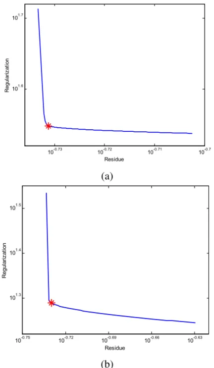
investi-gated, and it is based on the maximum curvature in the L-curve [14]. Figures 4a–4b show the L-curve for triangular test function using q = 0.5 and 2.0, respectively. The L-curve for semi-triangular test function is displayed in Fig-ures 5a–5b. The regularization parameterαis chosen at the corner of the L-curve.

10-0.73 10-0.72 10-0.71 10-0.7

101.87 101.89 101.91 101.93 101.95 101.97

Residue

R

e

g

u

la

ri

z

a

ti

o

n

(a)

10-0.75 10-0.72 10-0.69 10-0.66 10-0.63

101.2 101.3 101.4 101.5

Residue

R

e

g

u

la

ri

z

a

ti

o

n

(b)

Figure 4 – L-curve for triangular test function: (a)q=1.5; (b)q =2.5.

The numerical values for the regularization parameters estimated by Morozov’s and Hansen’s criteria are shown in Table 3.

(13)

semi-10-0.73 10-0.72 10-0.71 10-0.7 101.6

101.7

Residue

R

e

g

u

la

ri

z

a

ti

o

n

(a)

10-0.75 10-0.72 10-0.69 10-0.66 10-0.63

101.3 101.4 101.5

Residue

R

e

g

u

la

ri

z

a

ti

o

n

(b)

Figure 5 – L-curve for semi-triangular test function: (a)q =1.5; (b)q=2.5.

triangular test function. The best reconstruction was obtained usingq = 2.5, and the worst forq =0.5.

Retrieval of atmospheric temperature profile

(14)

Triangular function Semi-triangular function αMorozov αHansen αMorozov αHansen

q =0.5 0.0285 0.0011 0.0346 0.0040

q =1.5 0.0231 0.0008 0.0231 0.0010

q =2.0 0.0414 0.0040 0.0419 0.0040

q =2.5 0.0579 0.0040 0.0583 0.0050

Table 3 – Regularization parameter computed by test functions using Morozov’s dis-crepancy principle and Hansen’s criterion.

0 0.1 0.2 0.3 0.4 0.5 0.6 0.7 0.8 0.9 1 0 0.1 0.2 0.3 0.4 0.5 0.6 0.7 0.8 0.9 1 x In it ia l T e m p e ra tu re

0 0.1 0.2 0.3 0.4 0.5 0.6 0.7 0.8 0.9 1 0 0.1 0.2 0.3 0.4 0.5 0.6 0.7 0.8 0.9 1 x In it ia l T e m p e ra tu re (a) (b)

0 0.1 0.2 0.3 0.4 0.5 0.6 0.7 0.8 0.9 1 0 0.1 0.2 0.3 0.4 0.5 0.6 0.7 0.8 0.9 1 x In it ia l T e m p e ra tu re (c) (d)

Figure 6 – Reconstructions for triangular test function, withαdetermined by Hansen’s

(15)

0 0.1 0.2 0.3 0.4 0.5 0.6 0.7 0.8 0.9 1 0 0.1 0.2 0.3 0.4 0.5 0.6 0.7 0.8 0.9 1 x In it ia l T e m p e ra tu re (a) (b)

0 0.1 0.2 0.3 0.4 0.5 0.6 0.7 0.8 0.9 1 0 0.1 0.2 0.3 0.4 0.5 0.6 0.7 0.8 0.9 1 x In it ia l T e m p e ra tu re (c) (d)

Figure 7 – Reconstructions for semi-triangular test function, with α determined by Hansen’s criterion: (a)q=0.5; (b)q =1.5; (c) q=2.0; (d) q=2.5.

retrieval of temperature and humidity profiles from satellite radiance data became important for applications such as weather analyses and data assimilation in numerical weather predictions models.

(16)

data processing. Due to the difficulty of obtaining correct RTE solutions, several approaches and methods were developed to extract information from satellite data [25, 26, 27, 28]. The direct problem may be expressed by [29]

Iλ(0)=Bλ(Ts)ℑλ(ps)+

Z 0

ps

Bλ[T(p)]

∂ℑλ(p)

∂p d p, (20)

where Iλ is the spectral radiance, λis the channel frequency;ℑ is the layer to space atmospheric transmittance function, the subscripts denotes surface [12];

andBis the Planck function which is a function of the temperatureT (or pres-sure p):

Bλ(T)=

2hc2/λ5

[ehc/kBλT ₋1_] (21)

beinghthe Planck constant,cthe light speed, andkBthe Boltzmann constant. For

practical purposes, equation (21) is discretized using central finite differences:

Ii = Bi,s(Ts)ℑi,s +

Np

X

j=1

Bi,j +Bi,j−1

2

[ℑi,j− ℑi,j−1] (22)

with Ii ≡ Iλi(0), Nλ is the number of channels in the satellite, and Np is the

number of the atmospheric layers considered.

Some previous results have employed a generalization of the standard maxi-mum entropy principle (MaxEnt-0) for solving this inverse problem [7, 30]: the higher order entropy approach. The same strategy can be applied here. There-fore, the non-extensive entropy of order-γ is defined as

S_qγ ≡ k

q−1



1−

Np

X

i=1

r_iq



 ; ri =

Ti

PNp

i=1Ti

(23)

and

r=1γp (24)

where γ = 0, 1, 2, . . . , and1 is a discrete difference operator. The stan-dard MaxEnt-0 can be derived from (23) and (24) imposingγ =0 andq =1.

A small value should be added to the difference operator (say ς = 10−15_{) to}

(17)

Figures 8–10 present the atmospheric temperature retrieval achieved using ra-diance data from the High Resolution Radiation Sounder (HIRS-2) of NOAA-14 satellite. HIRS-2 is one of the three sounding instruments of the TIROS Oper-ational Vertical Sounder (TOVS). The results for the non-extensive MaxEnt-0 (for short: NE-MaxEnt-0) did not produce good results – Figure 8. However, results with NE-MaxEnt-1 and NE-MaxEnt-2 are compared to those obtained with MaxEnt-2 (such results have already been analysed against the profile com-puted by ITPP-5, a TOVS processing package [7] employed by weather service research centers throughout the world), and toin situradiosonde measurements.

10−1

100

101

102

103

180 200 220 240 260 280 300 320

Pressure (hPa)

Temperature (K) Radiosonde

Max−Ent−2 NE−Ent−0, q=0.5

Figure 8 – Reconstructions for temperature profile:q =0.0.

(18)

250–50 hPa, the best performance was obtained by the NE-MaxEnt-1, for the 700-500 hPa better result for the MaxEnt-0, and for the region 1000–750 hPa the NE-MaxEnt-2 (q =0.5) has presented the better inversion.

10−1

100

101

102

103

180 200 220 240 260 280 300 320

Pressure (hPa)

Max−Ent−2 NE−Ent−1, q=0.5

Conclusion

The implict strategy and the regularization techniques adopted in this work yield good results in reconstructing the initial condition of the heat equation and the atmospheric temperature profile.

(19)

regular-10−1

100

101

102

103

180 200 220 240 260 280 300 320

Pressure (hPa)

Max−Ent−2 NE−Ent−2, q=1.5 NE−Ent−2, q=0.8 NE−Ent−2, q=0.5

ization parameter calculated by the Morozov’s principle tends to over-estimate the value ofα. However, looking at Table 4, it is possible to realize that the parameterαcomputed by the Hansen’s criterion is closer to the optimum. Nev-ertheless, sometimes is hard to obtain the L-curve. One case specially difficult was found toq =2.5, for some values ofαwas not possible to obtain a solution (no convergence). A possible solution to convergence would be to change the deterministic optimizer by a stochastic one. Table 4 shows that an appropriated choice of the non-extentive parameter q can improve the reconstruction. Of course, other schemes for determining the regularization parameter can be used (see [31]).

(20)

E(fα−Morozov) E(fα−Hansen) E(fα−Morozov) E(fα−Hansen)

q =0.5 0.3994 0.3490 0.2400 0.1676

q =1.0 0.3151 0.1959 0.4056 0.1958

q =1.5 0.2599 0.1697 0.3205 0.1745

q =2.0 0.2370 0.1530 0.4379 0.1800

q =2.5 0.2561 0.1302 0.5959 0.2041

Table 4 – Estimation error computed with regularization parameter found by Morozov’s discrepancy principle and Hansen’s criterion.

Pressure RMS NE- NE- NE-

NE-(hPa) Max-Ent-2 MaxEnt-2 MaxEnt-2 MaxEnt-1 MaxEnt-0

q =1.5 q =0.5 q =0.5 q=0.5

50-0.1 13.248 13.553 13.646 9.598 10.483

250-50 7.442 8.395 8.723 5.818 11.038

500-250 5.216 5.405 5.508 5.532 10.730

700-500 1.283 1.623 1.817 1.478 2.481

1000-700 4.428 3.704 3.475 5.334 17.518

Table 5 – Root-mean-square for MaxEnt-2 and Non-extensive MaxEnt of first and second orders (NE-MaxEnt-1 and NE-MaxEnt-2).

et al. [10] was linked to a previous result of physical relevance related to the relaxation of two-dimensional turbulence [18]. There is no reason to restrict the regularization operator Sq atq = 0.5. Actually, the worse reconstructions for

the triangular test function were obtained usingS0.5!

(21)

A Some properties for the non-extensive thermostatiscs

A1: Non-extensive entropy:

Sq(p)=

k

q−1



1−

Np

X

i=1

pq_i



 . (25)

A2: q-expectation of an observable:

Oq≡ hOiq =

Np

X

i=1

pq_ioi . (26)

Properties

1. Ifq →1:

S1=k

Np

X

i=1

pilnpi , (27)

O1=

Np

X

i=1

piOi . (28)

2. Non-extensive entropy is positive: Sq ≥0.

3. Non-extensivity

Sq(A+B)=Sq(A)+Sq(B)+(1−q)Sq(A)Sq(B) (29)

Oq(A+B)=Oq(A)+Oq(B)+(1−q)

Oq(A)Sq(B)+OqSq(A)

. (30)

4. MaxSqunder constrain Oq =

P

i p q

iǫi (canonical ensemble):

pi =

1

Zq

[1−β(1−q)ǫi]1/(1−q) (31)

where the ǫi is the energy of statei, Oq = Uq is the non-extensive form to

the internal energy, and the normalization factor Zq (partition function), for

1<q <3, is given by

Zq =

π β(1−q)

1/2

Ŵ[(3−q)/2(q −1)]

Ŵ[1/(q−1)] . (32)

Forq =1 yields

(22)

Acknowledgment. Authors acknowledge the CNPq and FAPESP, Brazilian

agencies for research support. H.F. de Campos Velho also thanks to the Prof. Dr. João Batista da Silva (UFPA, Brazil) and Dra. Valeria Cristina Barbosa (LNCC, Brazil) for the usefull discussions and support.

REFERENCES

[1] A.N. Tikhonov and V.I. Arsenin, Solutions of Ill-posed Problems. John Wiley & Sons, 1977.

[2] E.T. Jaynes, Information theory and statistical mechanics.Phys. Rev.,106(1057), 620.

[3] C.D. Rodgers, Retrieval of the atmospheric temperature and composition from remote mea-surements of thermal radiation.Rev. Geophys. Space Phys.,14(1976), 609–624.

[4] C.R. Smith and W.T. Grandy (Eds.). Maximum-Entropy and Bayesian Methods in Inverse Problems, in Fundamental Theories of Physics, Reidel, Dordrecht (1985).

[5] F.M. Ramos and H.F. de Campos Velho, Reconstruction of geoelectric conductivity distribu-tions using a minimum first-order entropy technique, 2nd International Conference on Inverse Problems on Engineering, Le Croisic, France, vol. 2, 199 (1996).

[6] H.F. de Campos Velho and F.M. Ramos, Numerical inversion of two-dimensional geoelectric conductivity distributions from eletromagnetic ground data. Braz. J. Geophys.,15(1997),

133.

[7] F.M. Ramos, H.F. de Campos Velho, J.C. Carvalho and N.J. Ferreira, Novel Approaches on Entropic Regularization.Inverse Problems,15(5) (1999), 1139–1148.

[8] C. Tsallis, Possible generalization of Boltzmann-Gibbs statistics. J. Statistical Physics,

52(1988), 479.

[9] C. Tsallis, Nonextensive statistics: theoretical, experimental and computational evidences and connections.Braz. J. Phys.,29(1999), 1.

[10] L. Rebollo-Neira, J. Fernandez-Rubio and A. Plastino, A non-extensive maximum entropy based regularization method for bad conditioned inverse problems. Phys. A,261(1998), 555.

[11] W.B. Muniz, F.M. Ramos and H.F. de Campos Velho, Entropy- and Tikhonov-based regular-ization techniques applied to the backwards heat equation. Comp. Math. Appl.,40(2000),

1071.

[12] W.B. Muniz, H.F. de Campos Velho and F.M. Ramos, A comparison of some inverse methods for estimating the initial condition of the heat equation.J. Comp. Appl. Math.,103(1999), 145.

[13] V.A. Morosov,Methods for Solving Incorrectly Posed Problems. Springer Verlag (1984).

[14] P.C. Hansen, Analysis of discrete ill-posed problems by means of the L-curve. SIAM Rev.,

(23)

[15] F.M. Ramos, R.R. Rosa, C. Rodrigues Neto, M.J.A. Bolzan, L.D.A. Sa and H.F. de Campos Velho, Nonextensive statistics and three-dimensional fully developed turbulence. Phys. A,

295(2001a), 250.

[16] F.M. Ramos, C. Rodrigues Neto, R.R. Rosa, L.D. Abreu Sa and M.J.A. Bolzan, Generalized thermostatistical description of intermittency and nonextensivity in turbulence and financial markets.Nonlinear Anal.-Theor.,23(2001b), 3521.

[17] A. Plastino and A.R. Plastino, Tsallis’s entropy and Jaynes’ information theory formalism. Braz. J. Phys.,29(1999), 50.

[18] B.M.R. Boghosian, Thermodynamic description of two-dimensional Euler turbulence using Tsallis’ statistics.Phys. Rev.,E 53(1996), 4754.

[19] T. Reginska, A regularization parameter in discrete ill-posed problem.SIAM J. Sci. Comput.,

17(1996), 740.

[20] E04UCF routine, NAG Fortran Library Mark 17, Oxford, UK (1995).

[21] J.D. Hoffmann, Numerical Methods for Engineers and Scientists. McGraw-Hill, 1993.

[22] E. Issamoto, F.T. Miki, J.I. da Luz, J.D. da Silva, P.B. de Oliveira and H.F. de Campos Velho, An inverse initial condition problem in heat conduction: a neural network approach, Braz. Cong. on Mechanical Eng. (COBEM), Campinas (SP), Brazil, Proc. in CD-ROM – paper code AAAGHA, page 238 in the Abstract Book (1999).

[23] F.T. Miki, E. Issamoto, J.I. da Luz, P.B. de Oliveira, H. F. de Campos Velho and J.D. da Silva, A neural network approach in a backward heat conduction problem, Braz. Conference on Neural Networks, Proc. in CD-ROM, paper code 0008, pages 19–24, São José dos Campos (SP), Brazil (1999).

[24] E.H. Shiguemori, H.F. de Campos Velho and J.D.S. da Silva, Estimation of initial condition in heat conduction by neural network, in this Proceedings – ICIPE-2002, May 26-31, Angra dos Reis (RJ), Brazil.

[25] C.D. Rodgers, Retrieval of the atmospheric temperature and composition from remote mea-surements of thermal radiation.Rev. Geophys. Space Phys.,14(1976), 609–624.

[26] S. Twomey, Introduction to the matehmatics of inversion in remote sensing and interative measurements. Amsterdam, Elsevier Scientific, 1977.

[27] W.L. Smith, H.M. Woolf and A.J. Schriener, Simultaneous retrieval os surface and atmo-spheric parameters: a physical analytically direct approach.Adv. In Rem. Sens.,7(1985).

[28] M.T. Chahine, Inverse Problem in Radiative Transfer: determination of atmospheric param-eters.Jour. Atmos. Sci.,27(1970), 960.

(24)

[30] J.C. Carvalho, F.M. Ramos, N.J. Ferreira and H.F. de Campos Velho, Retrieval of Vertical Temperature Profiles in the Atmosphere Inverse Problems in Engineering (3ICIPE), Proceed-ings in CD-ROM, under paper code HT02 (see also in the internet: http://www.me.ua.edu/ 3icipe/fin3prog.htm) – Proc. Book: pp. 235-238, Port Ludlow, Washington, USA, June 13-18, UEF-ASME (2000).