www.atmos-meas-tech.net/8/3577/2015/ doi:10.5194/amt-8-3577-2015
© Author(s) 2015. CC Attribution 3.0 License.
A methodology for investigating dust model performance using
synergistic EARLINET/AERONET dust concentration retrievals
I. Binietoglou1, S. Basart2, L. Alados-Arboledas3,4, V. Amiridis5, A. Argyrouli6, H. Baars7, J. M. Baldasano2, D. Balis8, L. Belegante1, J. A. Bravo-Aranda3,4, P. Burlizzi9, V. Carrasco10, A. Chaikovsky11, A. Comerón12, G. D’Amico13, M. Filioglou8, M. J. Granados-Muñoz3,4, J. L. Guerrero-Rascado3,4, L. Ilic14, P. Kokkalis5,6, A. Maurizi15, L. Mona13, F. Monti15, C. Muñoz-Porcar12, D. Nicolae1, A. Papayannis6, G. Pappalardo13, G. Pejanovic16, S. N. Pereira10, M. R. Perrone9, A. Pietruczuk17, M. Posyniak17, F. Rocadenbosch12,18, A. Rodríguez-Gómez12, M. Sicard12,18, N. Siomos8, A. Szkop17, E. Terradellas19, A. Tsekeri5, A. Vukovic16,20, U. Wandinger7, and J. Wagner7
1National Institute of R&D for Optoelectronics, 409 Atomistilor Str., 77125, Magurele, Ilfov, Romania 2Earth Sciences Department, Barcelona Supercomputing Center,
Centro Nacional de Supercomputación (BSC-CNS), Barcelona, Spain
3Department of Applied Physics, Universidad de Granada, Granada, Spain
4Andalusian Institute for Earth System Research (IISTA – CEAMA), University of Granada, Granada, Spain 5National Observatory of Athens, Institute for Astronomy, Astrophysics, Space Applications and Remote Sensing
(NOA-IAASARS), Athens, Greece
6National Technical University of Athens, Physics Department, Laser Remote Sensing Laboratory, Zografou, Greece 7Leibniz Institute for Tropospheric Research, Leipzig, Germany
8Aristotle University of Thessaloniki, Faculty of Sciences, School of Physics, Thessaloniki, Greece 9Dipartemento di Fisica, Universitá di Lecce, Lecce, Italy
10Èvora Geophysics Centre, Èvora, Portugal
11Institute of Physics, National Academy of Sciences of Belarus, Minsk, Belarus 12Department of Signal Theory and Communications, Remote Sensing Laboratory,
Universitat Politècnica de Catalunya, Barcelona, Spain
13Consiglio Nazionale delle Ricerche, Istituto di Metodologie per l’Analisi Ambientale (CNR-IMAA),
Tito Scalo, Potenza, Italy
14Institute of Physics, Belgrade, Serbia
15Consiglio Nazionale delle Ricerche, Istituto di Scienze dell’Atmosfera e del Clima (CNR-ISAC), Bologna, Italy 16South East European Virtual Climate Change Center (SEEVCCC), Republic Hydrometeorological Service of Serbia,
Belgrade, Serbia
17Institute of Geophysics, Polish Academy of Sciences, Warsaw, Poland 18Institute of Space Studies of Catalonia (IEEC- CRAE), Barcelona, Spain 19AEMET, Barcelona, Spain
20Faculty of Agriculture, University of Belgrade, Belgrade, Serbia
Correspondence to:I. Binietoglou (ioannis@inoe.ro)
Abstract. Systematic measurements of dust concentration profiles at a continental scale were recently made possible by the development of synergistic retrieval algorithms using combined lidar and sun photometer data and the establish-ment of robust remote-sensing networks in the framework of Aerosols, Clouds, and Trace gases Research InfraStruc-ture Network (ACTRIS)/European Aerosol Research Lidar Network (EARLINET). We present a methodology for using these capabilities as a tool for examining the performance of dust transport models. The methodology includes con-siderations for the selection of a suitable data set and propriate metrics for the exploration of the results. The ap-proach is demonstrated for four regional dust transport mod-els (BSC-DREAM8b v2, NMMB/BSC-DUST, DREAM-ABOL, DREAM8-NMME-MACC) using dust observations performed at 10 ACTRIS/EARLINET stations. The obser-vations, which include coincident multi-wavelength lidar and sun photometer measurements, were processed with the Lidar-Radiometer Inversion Code (LIRIC) to retrieve aerosol concentration profiles. The methodology proposed here shows advantages when compared to traditional eval-uation techniques that utilize separately the available mea-surements such as separating the contribution of dust from other aerosol types on the lidar profiles and avoiding model assumptions related to the conversion of concentration fields to aerosol extinction values. When compared to LIRIC re-trievals, the simulated dust vertical structures were found to be in good agreement for all models with correlation values between 0.5 and 0.7 in the 1–6 km range, where most dust is typically observed. The absolute dust concentration was typically underestimated with mean bias values of −40 to −20 µg m−3at 2 km, the altitude of maximum mean concen-tration. The reported differences among the models found in this comparison indicate the benefit of the systematic use of the proposed approach in future dust model evaluation stud-ies.
1 Introduction
Desert dust is emitted from arid regions around the world, and in many cases it is the dominant aerosol type. Dust aerosols affect the radiation balance and temperature struc-ture of the atmosphere by interacting both with short- and long-wave radiation (Sokolik and Toon, 1996; Pérez et al., 2006b; Balkanski et al., 2007); they also affect cloud micro-physical properties and precipitation patterns by acting as cloud condensation and ice nuclei (DeMott et al., 2003; Karydis et al., 2011) and, due to their large spatial and tem-poral extent, have an important effect on climate (Rosenfeld et al., 2001). The main source regions of dust are located in northern Africa and western and central Asia, but due to the prevalent wind patterns they have significant impact on the air quality of Europe, North America, and East Asia, far
away from their sources, affecting the health of large popu-lations (Morman and Plumlee, 2014). Additionally, mineral dust aerosols are suspected to be an important source of solu-ble iron in the marine ecosystems and, thus, an important fac-tor of marine bio-production (Mahowald et al., 2010; Nick-ovic et al., 2013; Gallisai et al., 2014).
Given this complexity, dust models are an important tool for studying the complete dust cycle in the atmosphere. Such models simulate dust’s lifecycle, including production in arid regions, transport in the atmosphere, and wet and dry depo-sition (Tegen, 2003). These models simulate the complete 3-D fields of dust concentration and can be used to study the processes and sensitivities controlling the dust distribution and to compute regional and global budgets of dust. Dust models have been used, for example, to quantify the effect of dust on air quality of Mediterranean cities (Jiménez-Guerrero et al., 2008), to study the effects of dust on weather forecasts (Pérez et al., 2006b), and to quantify the impact of lofted dust particles on cloud formation (Klein et al., 2010; Solo-mos et al., 2011). To perform these simulations, models rely on the physical description of atmospheric processes, on the choice of parameterization, and on the tuning of individual components in the model; consequently, modeling outputs need to be regularly tested against in situ and remote sens-ing measurements to evaluate their performance. When used as a forecasting tool, models can assimilate remote sensing measurements to improve their forecasting skill (Benedetti et al., 2009; Sekiyama et al., 2010; Wang et al., 2014).
Dust model evaluations typically include a combination of surface concentration, deposition fluxes, and remote sensing measurements (e.g., Basart et al., 2012b; Gama et al., 2015). On the remote sensing side, evaluations typically rely on ob-served columnar aerosol properties. For example, a typical quantity used is aerosol optical depth (AOD) measured by the Aerosol Robotic Network (AERONET) photometers or satellite platforms such as the Moderate Resolution Imaging Spectroradiometer (MODIS) (e.g Pérez et al., 2011; Basart et al., 2012b). In these comparisons, the modeled dust vol-ume concentration is converted to dust optical depth using spherical particle approximation and a modeled size distri-bution. These evaluation attempts are limited by the contri-bution of non-dust aerosols, and so are restricted to cases or regions where dust is the dominant aerosol type (e.g., Basart et al., 2009; Cuevas et al., 2014). Usually, the dust vertical distribution is not examined even though it may affect the model performance in many aspects. An accurate represen-tation of dust vertical structure is needed to model dust trans-port and deposition processes, to capture the effects of dust-radiation and dust-cloud interactions, and to properly pro-duce air quality forecasts (e.g., Wang et al., 2014).
and such measurements have been used to examine dust model performance. Many such examinations have focused on a limited number of case studies (e.g., Pérez et al., 2006a; Uno et al., 2006; Müller et al., 2009; Heinold et al., 2009). In other studies, long-term observation of aerosol optical prop-erties have been compared with modeled dust optical pro-files. For example, Mona et al. (2014) have presented a sys-tematic examination of BSC-DREAM8b (Barcelona Super-computing Center – Dust REgional Atmospheric Model 8 bins) modeled dust distribution over Potenza, Italy, for the 2000–2012 period, using lidar-derived backscatter and ex-tinction profiles. Similarly, Gobbi et al. (2013) compared the lidar dust extinction profiles with those modeled by BSC-DREAM8b over Rome, Italy during the 2001–2004 period. Results from these studies indicate that the dust models ad-equately represented the vertical distribution of dust despite underestimating the total extinction profiles. However, these studies compare modeled dust properties to total aerosol properties, as they do not separate the contribution of dust from other atmospheric aerosols, like smoke and pollution. In most cases no comparison can be made in the Planetary Boundary Layer (PBL) where the load of fine anthropogenic aerosols is always expected to be high, especially in the ma-jority of measurement sites in Europe. Depolarization lidars can overcome this problem by separating dust to non-dust aerosol backscatter coefficient, based on known depolariza-tion ratios of dust and other aerosol types (Shimizu et al., 2004; Tesche et al., 2009) but these techniques have been used only in few model evaluation studies (e.g., Heinold et al., 2011).
An alternative strategy for dust model comparison is based on the conversion of lidar backscatter signals to total aerosol volume concentration using scattering simulations (e.g Barn-aba and Gobbi, 2001, 2002). Such an approach was used to examine the performance of three dust transport models us-ing 34 elastic lidar profiles over Rome, Italy, for the 2001– 2003 period (Kishcha et al., 2005, 2007).
Recently, a number of newly developed algorithms are us-ing the synergy of lidar and sun/sky photometer data to re-trieve dust concentration profiles (e.g., Ansmann et al., 2012; Lopatin et al., 2013; Chaikovsky et al., 2015). Such algo-rithms can separate the contribution of dust from that of other aerosol types, so they can be used to examine the dust model performances even in cases where the dust particles are mixed with smoke, for example. These products are based on indirect observation of the aerosol size distribution – in-stead of relying on a modeled size distribution – further im-proving the results. Up to now, the comparison of these algo-rithms with models has been restricted to single cases; for ex-ample, Tsekeri et al. (2013) presented a case study where the output of BSC-DREAM8b model was compared with dust concentration retrieved using the Lidar/Radiometer Inversion Code algorithm (LIRIC) over Athens, Greece, finding satis-factory agreement. These algorithms have been implemented
in many European lidar stations, opening new possibilities for dust observation on a continental scale.
In this paper, we propose a strategy for cross-examining modeled dust concentration profiles and profiles retrieved us-ing such lidar/sun-photometer synergy. As an example, we use an observation data set produced with the LIRIC al-gorithm. The recent implementation of LIRIC in many ad-vanced European Aerosol Research Lidar Network (EAR-LINET) remote sensing stations (Chaikovsky et al., 2012) allows the systematic examination of model performance in a wider geographical region. In this paper we present a gen-eral methodology for comparing measured and modeled ver-tical dust concentration, including the strategies that could be used, the caveats that should be taken care of, and suggest the appropriate metrics that could help explore the data set. Next, we apply this methodology to compare dust concentra-tion profiles retrieved at 10 European remote sensing sites to 4 European regional dust transport models.
The four models that participate in this inter-comparison are BSC-DREAM8b v2, Nonhydrostatic Multiscale Mete-orological Model on the B grid/Barcelona Supercomput-ing Center – Dust (NMMB/BSC-Dust), DREAMABOL, and Dust REgional Atmospheric Model – Nonhydrostatic Mul-tiscale Meteorological Model on the E grid – Monitoring Atmospheric Composition and Climate (DREAM8-NMME-MACC). All four models contribute to the Sand and Dust Storm Warning Advisory and Assessment System (SDS-WAS) that was established by the World Meteorological Organization (http://www.wmo.int/sdswas). The SDS-WAS aims to improve the present capabilities for reliable sand and dust storm forecasts; to do this it supports the development of comprehensive, coordinated and sustained observations and modeling capabilities of these events. The SDS-WAS con-sists of two regional nodes, one for northern Africa, the Mid-dle East and Europe (NA-ME-E) – set in Spain, and one in Asia – set in China; each of these nodes deals with both op-erational and scientific aspects related to atmospheric dust monitoring and forecasting. All the models participating in the present study contribute to the NA-ME-E regional node.
Remote sensing profiling measurements can be used to im-prove dust modeling efforts at three different levels: diagnos-tic evaluation, near-real-time (NRT) evaluation, and assimi-lation (Seigneur et al., 2000; Sicard et al., 2015; Wang et al., 2014). In this study, we focus on the diagnostic evaluation of the model performance. We choose to study an extended time and space period that gives us better representation of differ-ent meteorological conditions, dust transport paths, and mea-surement locations. However, the considerations and metrics presented here can also be applied to the NRT evaluation sce-nario.
of the cross-examination, and present the appropriate statis-tical indicators that can be used for future evaluation of dust models. Finally, in Sect. 4 we present the results obtained by applying this methodology to real measurements. In Sect. 5 we give conclusions and indicate directions for future work.
2 Algorithms and Models 2.1 Measurement networks
The systematic observation of the vertical distribution of dust on a continental scale is possible due to the development of regional lidar remote sensing networks in main dust out-flow regions like the European Aerosol Research Lidar Net-work (EARLINET, Pappalardo et al., 2014), the AD-Net in East Asia (Sugimoto et al., 2005), the Latin American Li-dar Network (LALINET) in Latin America (Barbosa et al., 2014; Guerrero-Rascado et al., 2014), and the global Mi-cropulse Lidar Network (MPLNET, Campbell et al., 2002). This study focuses on EARLINET, a lidar network that was established in 2000 with the aim of providing comprehen-sive information for the aerosol vertical distribution over Eu-rope (Bösenberg et al., 2001). Currently, 27 stations partici-pate actively in the network with regular contribution of data. The network includes 17 stations with multi-wavelength Ra-man systems, while 18 stations perform depolarization mea-surements, giving important information on the shape of the measured particles. All stations in the network perform cli-matological measurements – three times a week according to a predefined measurement schedule – together with ex-tra measurements in special events, dust measurements based on an alerting system, and intensive observational measure-ment campaigns (Pappalardo et al., 2014). Considerable at-tention has been given within EARLINET to improve and homogenize the performance of the systems, including hard-ware tests, algorithm tests on synthetic data, and system in-tercomparison campaigns (Matthias et al., 2004; Böckmann et al., 2004; Pappalardo et al., 2004). The optical products calculated from all the systems are stored in a standardized data format in a central database and are available for exter-nal users. The first volumes of the EARLINET database have been published in biannual volumes at the World Data Center for Climate (The EARLINET publishing group 2000–2010, 2014).
Similarly, regional-to-global sun/sky photometer networks like Aerosol Robotic Network (AERONET, Holben et al., 1998), Global Atmosphere Watch – Precision Filter Ra-diometer network (GAW-PFR, McArthur et al., 2003), Skyrad Network (SKYNET, Takamura and Nakajima, 2004; Kim et al., 2008), and the China Aerosol Remote Sensing Network (CARSNET, Che et al., 2009) have also been de-veloped. Many of these instruments are collocated with li-dar system of the corresponding lili-dar networks, thus allow-ing the development of synergistic algorithms. In this study,
we use AERONET, a global network of automatic sun/sky-scanning photometers that was created in the mid 90s in or-der to provide global aerosol data not provided at the time by satellites and to act as a validation platform for future satellite missions. Its current aim is to provide long-term, continuous measurements of columnar aerosol optical and microphysical properties. The network consists of standard-ized photometers produced by Cimel Electronique and all participating instruments undergo regular calibration and in-tercomparison with reference instruments. The photometers in the AERONET network perform both direct-sun and sky-scanning almucantar measurements at several wavelengths (between 340 and 1640 nm). The output of direct-sun mea-surements is the AOD in several wavelengths, while the sky-scanning measurements are also used for retrieving aerosol microphysical properties (Dubovik and King, 2000; Dubovik et al., 2006). The processing is centrally performed and the results are made public in near-real time.
2.2 Retrieval algorithms
As described in the introduction, a new class of algorithms can retrieve dust volume concentration profiles utilizing lidar profiling measurements and sun/sky photometer data. The output of these algorithms is the vertical concentration of a number of separate aerosol types. In these algorithms, dust microphysical properties are neither assumed a priori nor are derived from model outputs, but are based on photometer measurements or known properties of pure dust. In this way, they address a core issue of model evaluation from remote sensing measurements: dust transport models simulate mass concentration while the main measured quantities of remote sensing instruments are optical aerosol properties; a conver-sion is always necessary to make the two quantities compa-rable. When the conversion is made on the model side, the model’s mass concentration is converted to extinction pro-files using a predefined volume-to-extinction ratio. If the dust transport model treats the dust size distribution in a realistic way, e.g., separating the dust concentration in many different size bins, a better conversion can be achieved using forward scattering calculations (typically based on Mie theory). The use of the synergistic algorithms allows to directly compare the retrieved volume concentration profiles to model output, removing from our study an extra factor of uncertainty.
In this work, we will use the LIRIC algorithm as an ex-ample to demonstrate the proposed methodology. LIRIC is used in many European remote sensing stations and takes full advantage of the remote sensing networks EARLINET and AERONET. The results we present are, nevertheless, ap-plicable to similar data sets retrieved by other algorithms. Before presenting the algorithm’s details, we present a brief overview of this class of algorithms to make clear in what aspects LIRIC can be considered a representative example.
op-tical properties of some aerosol types to retrieve the concen-tration of these types in the atmosphere. The used aerosol intensive properties can be derived from past observations, laboratory measurements, model data or a combination of the above. When the range of such input values is too wide for a reliable retrieval, photometer measurements are sometimes used as a proxy for the missing parameter. For example, the polarization lidar photometer networking (POLIPHON) algorithm (Ansmann et al., 2011, 2012) is based on dust depolarization and extinction-to-backscatter coefficient ra-tio (aerosol lidar rara-tio) observed during the Saharan Min-eral Dust Experiment (SAMUM) and long-term EARLINET measurements of dust transport events over Europe. In ad-dition, POLIPHON uses the volume-to-AOD ratio derived from the photometer to approximate the variable volume-to-extinction ratio for dust and smoke aerosols. Extending this approach, Mamouri and Ansmann (2014) use laboratory measurements of fine and coarse dust depolarization ratio to further separate these two sub-classes of dust. In a similar ap-proach, Nemuc et al. (2013) derive the volume-to-extinction ratio of different aerosol types from the Optical Properties of Aerosols and Clouds (OPAC) database (Hess et al., 1998). Other approaches combining lidar measurements with air-borne measurements or complex AERONET processing have also been developed (Cuesta et al., 2008; Lewandowski et al., 2010).
The second category of algorithms pursues a more tight in-tegration of lidar and photometer data. Specifically, the vol-ume concentration profiles are calculated to optimally fit the lidar and photometer measurements (Dubovik, 2005). In the case of the Generalized Aerosol Retrieval from Radiome-ter and Lidar Combined data algorithm (GARRLiC, Lopatin et al., 2013), the optimal fit of the lidar and photometer measurements is found using a multi-term least square ap-proach. Similarly, LIRIC (Chaikovsky et al., 2015) uses the AERONET inversion products to derive the intensive proper-ties of fine and coarse aerosols; consequently, the algorithm finds the optimal profiles of these types based on lidar mea-surements and total-column volume concentration profiles provided by AERONET. The higher integration of the pho-tometer and lidar comes with a price. These algorithms re-quire simultaneous lidar and photometer measurements and this limits the available measurements, especially because photometer sky-scanning measurements require a cloud-free conditions and are performed only during daytime. They also typically require more complex lidar systems, performing multi-wavelength measurements, introducing limitations re-garding the lidar systems that they could be applied. More-over, simulating the complete atmospheric column makes the algorithms sensitive to the conditions near the ground, where typical lidar systems cannot observe. On the other hand, their benefit is that they can distinguish coarse spherical and non-spherical particles, separating, for example, dust from marine particles.
In this paper, we use results from the LIRIC algorithm to show the benefit of using such algorithms for dust model evaluation. The details of LIRIC can be found in Chaikovsky et al. (2004, 2012); Wagner et al. (2013); Chaikovsky et al. (2015) so only a brief overview is given here.
LIRIC uses as input elastic lidar signals at three wave-lengths (355, 532, 1064 nm) and aerosol microphysical prop-erties retrieved from the AERONET inversion algorithm. It can optionally use also depolarization measurements at 532 nm. LIRIC assumes that atmospheric particles can be separated in fine, coarse spherical, and coarse spheroid modes. It calculates the microphysical properties of these three modes using the AERONET retrieval of columnar size distribution, refractive index and sphericity. It separates the fine and coarse size distribution by finding the minimum con-centration values 0.194–0.576 µm range. The algorithm cal-culates the intensive properties (e.g., volume-to-extinction coefficient) at all lidar wavelengths using the same sphere and spheroid kernel functions as AERONET (Dubovik et al., 2006). Additionally, it calculates the total volume concentra-tion of each mode integrating the size distribuconcentra-tion and using the sphericity parameter to separate the coarse-mode volume to spherical and spheroid components. LIRIC assumes that the properties of these modes do not change with altitude, but the concentration of each modeCm(z)can vary freely. The algorithm uses as input pre-processed lidar signals. The signal time series is averaged to achieve good signal-to-noise ratio. The signals are normalized to a reference altitudezn and are also cut at the altitude of full overlapzO.
LIRIC finds the volume concentration profilesCm(z)for the three modes by optimizing (a) the fit to the lidar sig-nals, (b) the fit to the AERONET columnar volume con-centration, and (c) user-defined smoothness constraints that act as a regularization parameter. The relative importance of these three constraints is selected by the user through appro-priate weighting factors. The optimization is performed us-ing a multi-term least square algorithm. The concentration bellow the full overlap height is considered constant, i.e.,
Cm(z)=Cm(zO) for z < zO. LIRIC’s final output are the volume concentration profiles of fine, coarse spherical and coarse spheroid particles. If depolarization measurements are not available, the coarse mode is not separated in two com-ponents, and the final output is concentration of only fine and coarse modes.
re-trieves the coarse spheroid mode, and this could incorpo-rate more than one aerosol type if the atmosphere includes desert and volcanic dust, or even dust from two very differ-ent sources. These cases are rare and will have a small ef-fect in a statistical comparison. We cannot exclude, however, that they can become important for specific cases. Secondly, the aerosol complex refractive index and sphericity parame-ter are considered to be size-independent, i.e., the same for fine and coarse-mode aerosols. The effect of this assump-tion on the retrieved volume concentraassump-tion is not thoroughly studied, but has been addressed in the GARRLiC algorithm (Lopatin et al., 2013). Thirdly, LIRIC assumes that aerosol scattering properties can be represented by the AERONET spherical and spheroid kernels. This assumption could be problematic because the AERONET kernels were not devel-oped to represent the phase function at the backscattering direction. Less importantly, the spheroid particle aspect ra-tio is adapted to represent coarse-mode dust particles and could be inappropriate for fine-mode particles. The fourth assumption, as mentioned before, is that aerosol below the full overlap height,zO, are well mixed. This will not be true
if the PBL height is lower than this altitude. Consequently, the effect of this assumption will depend on the atmospheric condition and will be different from case to case. Finally, if the photometer and lidar measurements are not simultane-ous, the retrieval assumes that columnar intensive and exten-sive aerosol properties did not change between the measure-ments. Again, the effect of this variability will be different in each case but could be checked using available ancillary measurements e.g., from direct-sun photometer or collocated ceilometer (Wiegner et al., 2014; Madonna et al., 2014). Note that these assumptions will mostly affect the total value of the concentration profiles. The shape of the profile is mostly determined by lidar measurements of spectral dependence of the backscatter and the depolarization coefficient.
A full uncertainty analysis of LIRIC retrievals is still an open topic. The output of LIRIC has been validated against POLIPHON retrievals that do not rely on a specific aerosol model (Wagner et al., 2013); the comparison indicates that the spheroid model that represents non-spherical particles does not induce significant errors in the retrieval. A further source of uncertainties is the choice of user-defined parame-ters for each retrieval; such parameparame-ters include, for example, minimum and maximum altitude, the altitude of an aerosol-free region, and regularization parameters used in the inver-sion. Granados-Muñoz et al. (2014) show that the retrieval is stable to the choice of these parameters, but further work is needed to generalize these results; in the examples shown in that paper, the result retrieval errors remain below 20 %.
2.3 Dust models
Dust transport modeling was a point of intense research since the 1990s and several global and regional models have been developed (Tegen and Fung, 1994; Nickovic and Dobricic,
1996; Benedetti et al., 2014). In this study, we focus on regional transport models setup over the domain of North Africa and Europe; these models are frequently used to pre-dict dust transport over Europe and to explore the effects of dust in the European atmosphere.
As mentioned in the introduction, the four models used for the demonstration of the described methodology are BSC-DREAM8b v2, NMMB/BSC-Dust, DREAMABOL, and DREAM8-NMME-MACC. Being part of the SDS-WAS pro-gram, all models undergo near-real-time evaluation against satellite- and ground-based columnar observations.
The Dust Regional Atmospheric Model (DREAM; Nick-ovic et al., 2001) is based on the Euler-type partial dif-ferential nonlinear equation for dust mass continuity and is driven by NCEP/Eta. It assumes a viscous sublayer be-tween the smooth desert surface and the lowest model layer (Janjic, 1994; Nickovic et al., 2001). The updated version of the model is the BSC-DREAM8b v2 model (Pérez et al., 2006a, b; Basart et al., 2012b) which is devel-oped and operated at the Barcelona Supercomputing Cen-ter, Spain (BSC; http://www.bsc.es/projects/earthscience/ BSC-DREAM/). It includes a set of updates, such as an ap-proximation of the dust size distribution by 8 size bin, im-proved source representation, and updated wet and dry de-position schemes. The model has been extensively evalu-ated against observations (e.g., Pay et al., 2010; Basart et al., 2012b, a).
The DREAMABOL model is an online integrated regional mineral dust model developed at the Institute of Atmospheric Sciences and Climate, Bologna, Italy, as part of the atmo-spheric composition and meteorology model BOLCHEM (Mircea et al., 2008; Maurizi et al., 2011). The meteorologi-cal component is the BOLAM primitive equation hydrostatic model (Buzzi et al., 2003). The dust model part is inspired by DREAM (Nickovic et al., 2001) but is completely rewritten and includes different assumptions on the model source and on the wet removal (Maurizi and Monti, 2015). DREAM-ABOL provides data to the SDS-WAS since June 2014 and participates since then in the near-real-time evaluation.
The DREAM8-NMME-MACC is developed and operated at the South East European Virtual Climate Change Center (SEEVCCC; http://www.seevccc.rs/), Serbia. The DREAM8 model is embedded in the NCEP Nonhydrostatic Mesoscale Model (NMM) on the E-grid (Janjic et al., 2001), while ini-tial and boundary conditions are taken from ECMWF global forecast. This version of DREAM8 assimilates ECMWF dust analysis in the initial dust field, with dust sources defined from Ginoux et al. (2001). DREAM8-NMME-MACC pro-vides daily dust forecasts available at the SEEVCCC web-site.
Table 1.Summary of the main parameters of the dust transport models used in this study (adapted from Benedetti et al., 2014).
BSC-DREAM8b v2 NMMB/BSC-DUST DREAMABOL DREAM8-NMME-MACC Institution BSC-CNS BSC-CNS CNR-ISAC SEEVCCC
Meteorological driver Eta/NCEP NMMB/NCEP BOLAM NMME/NCEP Initial and boundary conditions NCEP/GFS NCEP/GFS NCEP/GFS ECMWF
Model domain 28◦W–68◦E, 0◦–70◦N 28◦W–68◦E, 0◦–70◦N 25◦W–60◦E, 0◦–65◦N 26◦W–62◦E, 7◦–57◦N
Resolution 0.33◦×0.33◦ 0.33◦×0.33◦ 0.4◦×0.4◦ 0.25◦×0.25◦
Boundary condition update 6 h 6 h 3 h 6 h
Source mask USGS-FAO with USGS-FAO with USGS-FAO with USGS-FAO with Ginoux et al. (2001) Ginoux et al. (2001) Ginoux et al. (2001) Ginoux et al. (2001) Emission scheme Uplifting
–Shao et al. (1993) –Janjic (1994) –Nickovic et al. (2001)
Saltation and sandblasting –White (1979)
–Marticorena and Bergametti (1995)
–Janjic (1994) –Nickovic et al. (2001)
Uplifting –Shao et al. (1993) –Nickovic et al. (2001)
Uplifting –Shao et al. (1993) –Janjic (1994) –Nickovic et al. (2001)
Deposition scheme Dry deposition –Zhang et al. (2001) Below-cloud scavenging –Nickovic et al. (2001)
Dry deposition –Zhang et al. (2001) Wet deposition –Ferrier et al. (2002) –Betts (1986) –Janjic (1994)
Dry deposition –Zhang et al. (2001) In and below-cloud scavenging
–Maurizi and Monti (2015) Convective clouds, precipitation and re-evaporation
Dry deposition –Zhang et al. (2001) Below-cloud scavenging –Nickovic et al. (2001)
Vertical resolution 24 Eta-layers 40σ-hybrid layers 50σ-hybrid layers 24σ-hybrid layers Transport size bins 8 (0.1–10 µm) 8 (0.1–10 µm) 8 (0.1–10 µm) 8 (0.1–10 µm) Radiation interaction Yes No No No
Data assimilation No No No Using MODIS-MACC initial fields
multi-scale atmospheric dust model fully embedded into the NMM on B-grid (Janjic et al., 2011). As with DREAM, this model assumes a viscous sublayer between the smooth desert surface and the lowest model layer while it includes a physi-cally based dust emission scheme, which explicitly takes into account saltation and sandblasting processes (White, 1979; Marticorena and Bergametti, 1995; Marticorena et al., 1997). The NMMB/BSC-Dust model has been evaluated at regional and global scales (Pérez et al., 2011; Haustein et al., 2012). It provides operational dust forecast for the Barcelona Dust Forecast Center (BDFC; http://dust.aemet.es/) the first spe-cialized center of the WMO for dust prediction.
While each model has a different setup, they use com-mon description of dust size distribution using eight size bins between 0.1 and 10 µm (Pérez et al., 2011) with intervals taken from Tegen and Lacis (1996) and Pérez et al. (2006a). Dust within each transport bin is assumed to have a time-invariant log-normal distribution (Zender et al., 2003) with the shape of the distribution fixed to a mass median diam-eter of 2.524 µm (Shettle, 1986) and a geometric SD of 2.0 (Schulz et al., 1998). The dust mass in each bin depends on model processes. Many other subcomponents are shared be-tween some of the models.
In the present analysis, various model output fields at 3-hourly resolution are compared. The research teams at the
modeling centers configured their model experiments inde-pendently and not necessarily following the setup of their re-spectively daily operational forecast. The spatial resolution, domain size, initial and boundary conditions all differ, as do the physical parameterizations implemented in the models summarized in Table 1.
3 Methodology
In this section we present the considerations for constructing the remote sensing data set and choosing statistical indica-tors that can be used for the model and measurement cross-examination. Special attention is given in selecting a repre-sentative data set, avoiding possible biases due to the geo-graphical restrictions of the measurement location, the selec-tion of vertical resoluselec-tion, and the effect of local dust sources in the study of the PBL. The considerations that guided our choices are given below.
se-lected algorithm. Thus, in the case of LIRIC, dust is as-sumed to be a particle component larger than ∼0.5 µm in
radius. On the other hand, the total dust load predicted by the models also includes smaller particle sizes in the first few bins of the dust size distribution. The contribution of these small particles in the total aerosol volume should be typi-cally low, especially near the source (d’Almeida, 1987; Ma-howald et al., 2014), but could become more important in few cases of long-range dust transport where the larger particles have been gravitationally removed (Mamouri and Ansmann, 2014). When using a statistical approach, including different locations and transport paths, as in the present study, these few cases are expected to have a small effect on the over-all comparison. The exact amount of fine-mode transported dust is an open issue and should be further investigated. The fine-mode contribution, however, is expected to be important when performing a case study evaluation, and then only spe-cific bins from the model output should be used instead.
In the case of statistical model evaluation, the selected measurement profiles should also be independent in order to give a correct representation of the model performance. Specifically, it should be avoided that the used measurements from each station sample the same event multiple times, but should instead measure independent dust transport events. This consideration is less important when using data from automatic instruments; in the case of EARLINET, however, the available data set could contain data from long observa-tions periods and intensive measurement campaigns, as de-scribed in Sect. 2.1. Ideally, only a climatological data set would be used, but the number of the available cases would be limited from the measurement frequency, the sporadic na-ture of dust transport episodes, and, when using synergistic algorithms, the availability of AERONET data. In this study, we consider to sample independent dust transport events by measurements that had at least 24 h time difference, com-patible with the expected variability of tropospheric aerosols (Anderson et al., 2003a, b).
The vertical resolution of lidar and dust model profiles should be taken into account during their comparison. The lidar signals have a raw vertical resolution of a few me-ters and the final products have an effective resolution of a few hundred meters depending on filtering procedures and smoothness constraints used in the retrieval (Pappalardo et al., 2004). The vertical resolution of the models, on the other hand, is typically coarser but depends on the vertical resolution of the meteorological driver (Simmons and Bur-ridge, 1981; Mesinger, 1984). When performing a statisti-cal comparison, the different vertistatisti-cal resolutions are less im-portant as the features of individual dust transport cases will be smoothed. When comparing aerosol extensive properties (both optical and concentrations) the remote sensing profiles should be upscaled to the model resolution. When, however, the aim of the comparison is to evaluate the dust-layer geo-metrical properties and values at a specific location, e.g., the peak concentration values, the finer resolution remote
sens-ing profiles should be used. In this study and in order to fa-cilitate the comparison of models of different vertical res-olutions, we interpolate all available profiles to a common 100 m vertical resolution. We used this resolution to examine the geometrical properties and peak concentration value of dust layers, but used 500 m averages to calculate the statis-tics on the vertical profiles presented in the next section. The models simulate the dust concentration profiles on a speci-fied horizontal grid, so bilinear interpolation was used to es-timate the concentration values at the exact location for each station. Linear interpolation was also utilized to estimate the concentration profiles at the exact time of the available mea-surements.
Correct representation of the dust mixing in the PBL can impact the forecasted air quality and also affect the removal processes of dust in the model. In this process, dust is mixed with locally produced aerosols, so lidar optical profiles can-not be used to directly study the dust effect. The mass re-trieval algorithms, like LIRIC, are able to separate the dust component in the PBL and give some insights to study this process, even though several limitations remain. Firstly, lo-cal dust sources could contribute to the dust load in the PBL (Korcz et al., 2009), although the exact effect of such sources to the vertical dust distribution, to our knowledge, has not been systematically studied. Secondly, as dust comes in con-tact with other types of particles and high relative humidity, some of the assumptions of the retrieval algorithms could be invalid. For example, it is reasonable to assume that polluted and humid PBL will lead to dust being coated and water layer to form on the dust particles, changing their optical proper-ties (Levin et al., 1996; Kumar et al., 2011b; Perry et al., 2004). Such effect could be important for the exact quantita-tive characterization of dust but does not completely prevent studying the mixing of dust in the PBL. Lastly, most lidar systems have a high overlap function and can only detect the initial mixing of dust in the upper parts of the PBL. Given these factors, the study of this mixing process could be done better for specific case studies. If a statistical approach is fol-lowed, the data set should be large enough to give significant results, as only few profiles cannot capture this dynamical mixing phenomenon.
0 20 40 60 Normalized signals [a.u] 0
2 4 6 8
A
lt
it
u
d
e
a
.s
.l
[k
m
]
LIDAR
355nm 532nm 1064nm 532nm-C
10−1 100 101
r[µm]
0.00 0.02 0.04 0.06 0.08
d
V
(
r
)
/
d
ln
(
r
)
[
µ
m
3/
µ
m
2]
Fine Coarse
AERONET
0 10 20 30 40 50 Volume concentration
[µm3 /cm3
] 0
1 2 3 4 5 6 7 8
A
lt
it
u
d
e
a
.s
.l
[k
m
]
LIRIC
Fine
Coarse/Spherical Coarse/Spheroid
0 40 80 120 160
Mass concentration [µg/m3
]
LIRIC MODEL
C [g/m2
] 0.21 0.20
CoM [km] 3.70 3.69
P [µg/m3
] 121.00 87.86
l [km] 5.10 4.60
Profile
r 0.91
FB 0.36 Comparison
DREAMABOL LIRIC
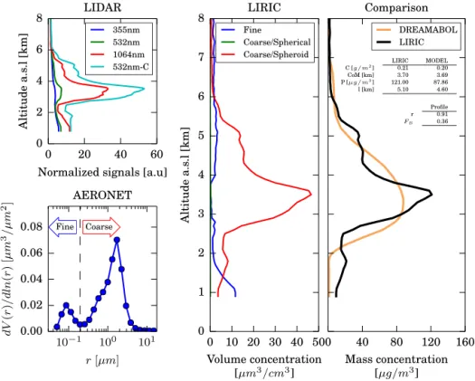
Figure 1.A sketch of the data processing procedure. Data are from Potenza, Italy (40.60◦E, 15.72◦N) at 11 April 2011. Left plots: LIRIC input i.e., normalized lidar signals (top) and AERONET microphysical inversion (bottom). The vertical line indicates the split between fine and coarse mode. Center plot: volume concentration profiles retrieved by LIRIC. Coarse spherical mode is near zero for all altitudes. Right plot: comparison of the mass concentration profile from LIRIC and DREAMABOL. The embedded tables give the point and profile statistics.
We perform the comparison firstly by examining single statistical indicators of each measurement case and secondly looking into indicators at different altitude ranges. This ap-proach allows assessing both the total performance of the models and the detailed performance across the profile. The single parameters examined are center of mass, total concen-tration, peak concentration value, and dust-layer thickness. For the profile parameters, apart from the average profiles, we examine the mean bias error, correlation coefficient, root mean square error, and fractional gross error. This set of pa-rameters was chosen because it can provide a detailed view of performance while remaining compatible, as much as pos-sible, with the metrics already in use in the SDS-WAS colum-nar evaluation.
An important indicator for model vertical profiles is the center of mass (CoM), a parameter that gives in a single num-ber an indication of the altitude of the dust distribution. In cases were a single aerosol layer is present in the atmosphere, the CoM gives an indication of its mean altitude; in case of multiple layers, however, the CoM could be located in areas without any considerable dust load (Mona et al., 2006, 2014). The second single-value measure to compare is the dust total concentration, C, calculated across the altitude range
where both measured and model profiles provide valid re-sults. In this way, this comparison will be a little different
than comparing directly columnar measurements, as in the case of comparing photometer and total column model val-ues. In the latter case the used range includes the lower few hundred meters of the profile, thus including the contribution of local dust sources to the total column aerosol load, possi-bly producing a bias in the measurements.
A third metric examined is the peak value of the profile,
P. In cases where the main dust mass is located near the
ground, the lidar system can fail to detect the true maximum, and instead show a maximum value at the lowest point of the profile, i.e., the first point of full overlap. In these cases we considered as maximum value the first lofted layer peak, located as the first peak after the first local minimum of the concentration profile.
The forth metric examined is the dust-layer thickness,l.
It is defined here as the region where dust concentration ex-ceeds a certain limit, here chosen at 5 µg m−3. In previous studies the layer thickness was defined using the derivative of the lidar signal (e.g., Mona et al., 2014). We use a thresh-old approach to overcome limitations related to smoothing included in many volume retrieval algorithms.
Based on these metrics, we qualify the performance of each model by calculating the correlation coefficientr and
fractional biasFBfor all the available cases. To make values
these values. Specifically, for each point we calculate the dif-ferences between model and observations and exclude points where the difference is more than 4 standard deviations from the mean value.
Figure 1 sketches the steps used to preform the comparison of a model and an observation profile. The example measure-ments were performed at Potenza, Italy (40.60◦E, 15.72◦N) on 11 April 2011, when a strong lofted dust layer was ob-served at 3–5 km. The LIRIC retrieval is performed based on input of raw lidar signals and AERONET microphysi-cal retrieval (left plots). The retrieval outputs are volume concentration profiles for fine, coarse spherical, and coarse spheroid modes (center plot). In this specific case, the coarse spherical mode concentration is almost zero at all altitudes. Dust mass concentration profiles are calculated using the re-trieved coarse spheroid mode concentration and assuming bulk dust density of 2.6 g cm−3. These profiles are compared with model profiles that are interpolated at the station loca-tion using linear interpolaloca-tion at the exact time and space (right plot). The right panel of the figure includes the de-scribed statistical indicators that summarize the similarities and differences of the two profiles.
Profile statistical indicators are calculated by first averag-ing the compared profiles at 500 m resolution then comput-ing a set of statistics for each altitude range. This resolution was chosen as a trade-off between detailed aerosol structure and the signal noise of the lidar measurements. This value, however, needs to be determined in each study based on the number of available profiles. Apart from the mean value pro-files, the first set of metrics used are the mean bias and the root mean square error (RMSE); being expressed in units of concentration, these values are suitable for the intercompar-ison of models but can be misleading for the performance of models with altitude. In addition, RMSE is strongly dom-inated by the largest values, due to the squaring operation, so in cases where prominent outliers occur, RMSE becomes less useful and its interpretation more difficult. These lim-itations are addressed using a second set of statistical indi-cators, including correlation coefficient, fractional bias, and fractional gross error. Fractional bias is a normalized mea-sure of the mean bias and indicates only systematic errors which lead to under/over-estimation of the measured values. Similarly, the fractional gross error is a positively defined in-dicator that gives the same figure with respect to under- and over-estimation. Definitions of the used statistical indicators are given in Table 2.
4 Results and discussion
In this section we apply the described methodology to simu-lations performed by the four models described in Sect. 2.3. The aim is not to perform a full model evaluation. As de-scribed in the introduction, this would require the use of a set of complementary remote sensing and in situ
measure-Figure 2.Map of the ACTRIS/EARLINET remote sensing stations providing data for testing the proposed methodology.
ments. Instead this section aims to demonstrate the potential of the new concentration retrieval algorithms in future model evaluation activities.
Ten European remote sensing stations contributed data to this intercomparison, mainly concentrated in the Mediter-ranean area, as shown in Fig. 2. Their location and the data supplied can be seen in Table 3. All stations are part of the EARLINET and AERONET networks, a fact that guaran-tees that the provided data are of uniform quality. The par-ticipating stations provided, in total, 55 LIRIC retrievals of dust profiles for an agreed time period from January 2011 to February 2013. The number of measurements is limited by the sporadic nature of dust transport events, the requirement for simultaneous lidar and AERONET observations, and the available manpower for manual analysis of each case. Each station selected the cases and performed the LIRIC retrievals independently, based on the available measurements. For each station, the selected profiles were screened for having at least 24 h time distance, as described before, to consider only measurements of different dust transport events. The time difference between lidar and photometer measurements was kept as small as possible (65 % –<1 h, 87 % –<3 h). In
measure-Table 2.Definition, symbol, value range, and ideal score for the statistical performance indicators used in the systematic examination of dust model concentration profiles.cdenotes the concentration at altitudez.MiandOirepresent modeled and observed profiles, respectively for theith measurement pair. Altitude dependence is omitted for brevity.
Metric Symbol Definition Range Perfect score
Center of mass CoM
Rzmax zminz·c·dz Rzmax
zmin c·dz
– –
Mean bias MB 1
N XN
i=1(Mi−Oi) −∞–∞ 0
Correlation coefficient r
PN
i=1 Mi−M
Oi−O
h PN
i=1 Mi−M 2PN
i=1 Oi−O 2i
1 2
−1–1 1
Root mean square error RMSE
1 N
XN
i=1(Mi−Oi)
2
1 2
0–∞ 0
Fractional bias FB 2
N XN
i=1
Mi−Oi Mi+Oi
−2–2 0
Fractional gross error FE 2
N XN
i=1
Mi−Oi Mi+Oi
0–2 0
Table 3.The following 10 stations provided dust concentration profiles retrieved by the LIRIC algorithm. Three measurements of the Évora station do not include depolarization information. The provided references give further information for each station and the measurement instruments.
Station Location (◦N,◦E) Altitude (m) Lidar channels No. of profiles Reference
Athens 37.97, 23.77 212 3β 3 Kokkalis et al. (2012)
Barcelona 41.39, 2.17 115 3β 7 Kumar et al. (2011a)
Belsk 51.84, 20.79 180 3β 1 Pietruczuk and Chaikovsky (2012)
Bucharest 44.35, 26.03 93 3β+1δ 5 Nemuc et al. (2013)
Évora 38.57,−7.91 293 3β+1δ∗ 17 Preißler et al. (2011)
Granada 37.16,−3.61 680 3β+1δ 8 Guerrero-Rascado et al. (2009)
Lecce 40.30, 18.10 30 3β+1δ 1 Perrone et al. (2014)
Leipzig 51.35, 12.43 90 3β+1δ 3 Althausen et al. (2009)
Potenza 40.60, 15.72 760 3β+1δ 7 Madonna et al. (2011)
Thessaloniki 40.63, 22.95 60 3β 3 Papayannis et al. (2012)
ments or the lidar Raman extinction retrieval if available. A similar check was performed for the aerosol fine-mode frac-tion (FMF), to detect possible change in aerosol mixture. In all cases, FMF was kept below 20 % and the average differ-ence of the data set is 0.44 %, as shown in the second panel of Fig. 3. These values indicate that, in average, the AOD and FMF changes are not expected to introduce any bias in the data set. Additionally, for each case we performed back-trajectory analysis for both photometer and lidar measure-ments and checked qualitatively for any significant changes in the air-mass origin. All inversions were made using ei-ther level 1.5 (cloud-screened) or level 2 (cloud-screened and quality-assured) AERONET data. We have used photome-ter measurements with AOD greaphotome-ter than 0.1 at 440 nm, as shown in the right panel of Fig. 3. This value is lower than the AERONET level 2 quality limit, nevertheless we used the value as a compromise to allow the study of weaker dust transport events.
30 20 10 0 10 20 30 AOD difference [%] 0
2 4 68 10 12 14
No. Cases
0.36 % a)
20 10 0 10 20
FMF difference [%] 0
2 4 68 10 12 14 16
0.44 % b)
0.1 0.2 0.3 0.4 0.5 0.6 0.7 AERONET AOD at 440nm 0
2 4 6 8
10 c)
Figure 3.Quality analysis of the LIRIC data set:(a)difference of AOD between lidar and photometer measurements,(b)difference of fine-mode-fraction between lidar and photometer measurements,(c)histogram of photometer AOD for all cases. The red lines in(a)and(b) indicate the mean value of the data set.
2 4 6 8 10 12
Month 0
2 4 6 8 10 12 14 16
No. Profiles
a)
0 10 20 30 40 50 60
Number of measurements 0
2 4 6 8 10
Altitude a.s.l [km]
b)
Figure 4. Number of available measurements(a)per month and (b)per altitude.
simulated aerosol burden, an observational strategy with sys-tematic measurements should be followed. The four exam-ined dust transport models were run for the given period and the output was stored for 3 h intervals.
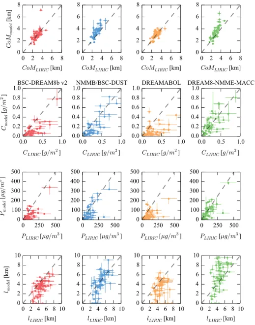
The comparison based on center of mass (CoM) reveals that models correctly track the main vertical location of transported dust. The first row of Fig. 5 presents this com-parison for the four models, and shows that the models per-form well when simulating the dust CoM in almost all cases. The difference of predicted and measured CoM exceeds 1 km only in 2 cases (4 %) for BSC-DREAM8b v2, 3 cases (5 %) for DREAMABOL, 8 cases (15 %) for NMMB/BSC-DUST, and 6 cases (11 %) for DREAM8-NMME-MACC. The BSC-DREAM8b v2 and DREAMABOL models show almost zero bias tracking the location of dust almost perfectly, except in few outlying cases. These are cases where the model prac-tically does not predict the transport event, and the CoM is determined by some residual concentration in the profile. In-stead, NMMB/BSC-DUST and DREAM8-NMME-MACC overestimate the center of mass altitude, especially in cases with observed CoM above 3 km; the fractional bias values for NMMB/BSC-DUST and DREAM8-NMME-MACC are 0.16 and 0.14 respectively. The correlation coefficient, values for the four models are 0.67 for BSC-DREAM8b v2, 0.81 for
DREAMABOL, and 0.74 for NMMB/BSC-DUST, and 0.83 for DREAM8-NMME-MACC.
Our examination indicates that four models simulate sys-tematically lower total amount of dust relatively to the LIRIC profiles. The second row of Fig. 5 presents the comparison of the dust concentration integrated across the common alti-tude range for each case. The mass concentration from the four models shows significant correlation with the measured one, but in general it is underestimated. For high concentra-tion cases (values greater than∼0.3 g m−2) NMMB/BSC-DUST and DREAM8-NMME-MACC predict sufficiently well the concentration values, while the other two models tend to underestimate. For low concentration values (less than 0.3 g m−2) all models apart from DREAM8-NMME-MACC underestimate the dust concentration in many cases. This could be caused by insufficient dust source strength, overestimated deposition and wet scavenging parameters, or a combination of both; the current data set is not sufficient to discriminate the exact factor affecting the comparison from the model point of view. It is believed, however, that using the present approach as part of a complete, multi-sensor eval-uation exercise would help investigating possible model lim-itations. The improved performance of DREAM8-NMME-MACC could be attributed to the assimilation scheme used only by this model. The total fractional bias values for the models range from−1.00 to−0.22, while correlation
coeffi-cients range from 0.51 to 0.83.
The third row of Fig. 5 shows the relationship of peak sim-ulated values for each profile and the measured ones. Also in this case, the models underestimate the maximum value of each profile. The fractional bias for the four models ranges from−0.85 to−0.27, while the correlation coefficient has
0 2 4 6 8
CoM
LIRIC [km] 0 2 4 6 8Co
M
mo de l [km ]0 2 4 6 8
CoM
LIRIC [km] 02 4 6 8
0 2 4 6 8
CoM
LIRIC [km] 02 4 6 8
0 2 4 6 8
CoM
LIRIC [km] 02 4 6 8
0.0 0.5 1.0
CLIRIC [g/m
2]0.0 0.2 0.4 0.60.8 1.0
C
model
[
g/m
2 ]
BSC-DREAM8b v2
0.0 0.5 1.0
CLIRIC [g/m
2]0.0 0.2 0.4 0.60.8
1.0NMMB/BSC-DUST
0.0 0.5 1.0
CLIRIC [g/m
2]0.0 0.2 0.4 0.60.8
1.0DREAMABOL
0.0 0.5 1.0
CLIRIC [g/m
2]0.0 0.2 0.4 0.60.8 1.0 DREAM8-NMME-MACC
0 250 500
PLIRIC [µg/m
3]0 100 200 300 400 500
P
model
[
µg/m
3]
0 250 500
PLIRIC [µg/m
3]0 100 200 300 400 500
0 250 500
PLIRIC [µg/m
3]0 100 200 300 400 500
0 250 500
PLIRIC [µg/m
3]0 100 200 300 400 500
0 2 4 6 8 10
l
LIRIC [km] 02 46 8 10
l
model
[km
]
0 2 4 6 8 10
l
LIRIC [km] 02 46 8 10
0 2 4 6 8 10
l
LIRIC [km] 02 46 8 10
0 2 4 6 8 10
l
LIRIC [km] 02 46 8 10
Figure 5.Comparison of single statistical indicators (rows) for the four models (columns) against LIRIC retrievals. First row shows the center of mass (CoM), second row the total concentration (C), third row the peak concentration (P), and fourth row the dust-layer thickness
(l). The model error bars represent the value for−3 and+3 h from the time of measurements. LIRIC error bars show indicative values of
error 30 % for concentration, 10 % for center of mass, 30 % for peak concentration, and 20 % for dust-layer thickness. These values are only approximate as the full characterization of LIRIC uncertainties is still an open issue.
The last row of Fig. 5 compares the dust-layer thickness parameter, i.e., regions where dust concentration is above 5 µg m−3. All models show good performance in predict-ing the dust layer, but there are individual differences. The DREAM8bV2 and DREAMABOL models systematically underpredict the dust-layer thickness, probably due to the un-derrepresentation of dust concentration. DREAM8-NMME-MACC systematically overpredicts the dust-layer thickness, as spreads the observed dust in higher altitude and in many cases does not reproduce correctly the top-layer boundary. The effect of our sampling strategy (only cases with observed dust) is apparent in the low values of these plots: in several
cases the models do not predict dust transport while we miss the cases were models predict dust when none is observed. The fraction bias ranges from−0.45 to 0 and the correlation
coefficient from 0.56 to 0.70. A summary of the
aforemen-tioned statistical indicators for all the examined models is given in Table 4.
Table 4.Correlation coefficient (r) and fractional bias (FB) for single value metrics of the compared profiles.
Center of mass Total concentration Peak value Layer thickness
r FB r FB r FB r FB
BSC-DREAM8b v2 0.67 0.00 0.81 −0.86 0.74 −0.85 0.68 −0.45
NMMB/BSC-DUST 0.81 0.16 0.83 −0.72 0.77 −0.68 0.70 −0.36
DREAMABOL 0.74 0.02 0.51 −1.00 0.61 −0.83 0.59 −0.55
DREAM8-NMME-MACC 0.83 0.14 0.74 −0.22 0.78 −0.27 0.56 −0.00
200 100 0 100 200 FB [%]
1.0 0.5 0.0 0.5 1.0
r
BSC-DREAM8b v2
200 100 0 100 200 FB [%]
1.0 0.5 0.0 0.5 1.0
r
NMMB/BSC-DUST
200 100 0 100 200 FB [%]
1.0 0.5 0.0 0.5 1.0
r
DREAMABOL
200 100 0 100 200 FB [%]
1.0 0.5 0.0 0.5 1.0
r
DREAM8-NMME-MACC
Figure 6.Scatter plot of vertical correlation and fractional gross error. Black dots represent the ideal performance (0, 1). Each point on the plot corresponds to a pair consisting of one LIRIC and one model profile. The error bars represent the value for model profiles−3 and+3 h
from the time of measurements. The bars on the axis indicate the univariate distribution of the data for each variable.
comparison. For each model-measurement pair we calcu-late the vertical correlation coefficient of the volume con-centration profiles as well as the fractional bias, and the re-sults are plotted in a scatterplot. We assess the model vari-ability for each case by calculating the same parameters for model profiles at −3 and+3 h of the observations, and depict the range of values with the error bars. The ideal model would have correlation one, i.e., it would predict per-fectly the shape of the dust profile, and 0 fractional bias, i.e., predicting correctly the quantity of transported dust. While individual cases show a big variability, each model shows a characteristic pattern. For BSC-DREAM8b v2 and DREAMABOL most cases have high correlation but neg-ative fractional bias i.e., the models can often predict cor-rectly the shape of the dust profile but underestimate the con-centration. In contrast, NMMB/BSC-DUST and DREAM8-NMME-MACC have fractional bias value distribution near 0
but a wider spread of correlation values. For all models there is a considerable spread of values for the specific compar-isons, a further argument for the need for a statistical evalua-tion of dust model performance.
These results are further supported by directly comparing the profile data provided by the model, indicating that mod-els do not only capture the general altitude of dust transport but, on average, predict correctly the shape of the dust pro-file. In Fig. 7 the mean measured concentration profile for all 55 cases is compared with the corresponding profiles of the four models. The profiles show good agreement in the pre-dicted shape of the dust concentration, but have wider spread in the absolute values. BSC-DREAM8b v2 and DREAM-ABOL predict the maximum dust concentration in the region 2–3 km a.s.l., in agreement with the observations, while the
0
20
40
60
80
100
Mass concentration [
µg/m
3]
0
2
4
6
8
10
Altitude a.s.l [km]
BSC-DREAM8b v2 NMMB/BSC-DUST DREAMABOL DREAM8-NMME-MACC LIRIC
Figure 7.Average profile comparison as simulated by four models and retrieved by LIRIC. Shaded areas indicate the standard devia-tion of the mean values.
the concentration of dust in altitudes above∼5 km; specifi-cally, while the observed values of dust are below 10 µg m−3 above 6 km, the model predicts these values only above 8 km. The concentration values show wider discrepancy: while the peak value of the mean profiles is retrieved at∼65 µg m−3 the models peak values range from ∼30 to ∼50 µg m−3. The observed increased concentration at high altitudes in some models could be related to misrepresentation of the tropopause (Janjic, 1994; Mona et al., 2014) that normally limits the maximum altitude of dust transport. In higher al-titudes, the main removal mechanism of dust is sedimenta-tion, and the removal of any dust reaching high altitudes is slower, allowing the artificial accumulation of dust. When examining the profile data, we can observe the differences in high and low concentration cases that were described be-fore, as shown in Fig. 8. NMMB/BSC-DUST and DREAM8-NMME-MACC have particularly good agreement at the high concentration cases. As noted before, such findings highlight the importance of statistical comparison approach and indi-cate that this trend should be investigated in a future complete evaluation study.
The above results are further explored in Fig. 9. The top left panel presents the mean bias of the four studied models. All models show negative bias below 4 km while above that altitude NMMB/BSC-DUST has almost 0 bias and DREAM8-NMME-MACC has positive bias values. At the altitude range where most dust is located, i.e., from 2 to 4 km a.s.l., the biases range from−46 to−5 µg m−3. Such bias is compatible with similar comparison again lidar ex-tinction profiles (Mona et al., 2014) and in the same direction as the model evaluation performed against AERONET and MODIS AOD measurements in the SDS-WAS NA-ME-E re-gional center (http://sds-was.aemet.es/). The top right panel shows the variation of the RMSE with altitude. In the 2–4 km
0 10 20 30 40 50 60
Mass concentration [
µg/m
3]
0
2
4
6
8
10
Altitude a.s.l [km]
Low concentration
0
50 100 150 200
Mass concentration [
µg/m
3]
0
2
4
6
8
10
High concentration
BSC-DREAM8b v2NMMB/BSC-DUST DREAMABOL DREAM8-NMME-MACC LIRIC
Figure 8. Comparison of average profiles simulated by all four models for low and high concentration cases, separated at 0.3 g m−2. Shaded areas indicate the standard deviation of the mean
values.
range, the mean values range from 40 to 70 µg m−3, with the maximum value reached by DREAMABOL at 2 km a.s.l.
The profiles of the correlation coefficient for the four mod-els are shown in the bottom left panel. All four modmod-els show significant correlation for altitudes ranging from 1 to 6 km, which is the region where most dust particles are typically observed (Mona et al., 2006). The mean values range from 0.52 for DREAMABOL to 0.68 for NMMB/BSC-DUST. Fi-nally, the bottom right panel shows the fractional gross er-ror profiles. The minimum values forFE, ranging from 0.73
to 1.09, are observed at 2–4 km. At higher altitudes, theFE
values are higher, with values ranging from 1.18 to 1.56 at 6 km a.s.l.
A summary of the different behavior of the four models is given in Fig. 10 using Taylor diagrams (Taylor, 2001). The data of the models and measurements were averaged at 1 km thick altitude bins (from 1 to 2 km, from 2 to 3 km etc.) before calculating the statistics, to give an overview of the model performance at different altitudes. Four Tay-lor diagrams are presented, for the altitude range from 1 to 5 km. DREAM8-NMME-MACC seems to capture correctly the range of values of the dust events in all altitude ranges, a property that can partly be attributed to the use of data as-similation. NMMB/BSC-DUST shows similar good perfor-mance, especially for 3 to 5 km. As observed before, the other two models underestimate the variability of dust in a consis-tent way with altitude. The model simulations have correla-tions from 0.4 to 0.8 at all four altitude ranges.
60 40 20 0 20 40 60 MB [µg/m3]
0 2 4 6 8 10
Altitude a.s.l [km]
a)
0 20 40 60 80 100
RMSE [µg/m3]
0 2 4 6 8
10 b)
BSC-DREAM8b v2 NMMB/BSC-DUST DREAMABOL DREAM8-NMME-MACC
1.0 0.5 0.0 0.5 1.0
r 0
2 4 6 8 10
Altitude a.s.l [km]
c)
0.0 0.5 1.0 1.5 2.0
FE
02 4 6 8
10 d)
Figure 9.Comparison of profile statistics for the four models against LIRIC measurements.(a)Mean bias,(b) root mean square error, (c)correlation coefficientr,(d)fractional gross errorFE. Gray shading indicates altitude ranges with less than 15 profiles available.
0.0 0.2 0.4
0.6
0.8 0.9
0.95
0.99 Correlation
0 8 16 24 32 40 48 56 64 72 0
8 16 24 32 40 48 56 64 72
Standard deviation
75
15
45
60
30
1 - 2km
0.0 0.2 0.4
0.6
0.8 0.9
0.95
0.99 Correlation
0 10 20 30 40 50 60 70 80 90 0
10 20 30 40 50 60 70 80 90
Standard deviation
20 100
60 40
80
2 - 3km
0.0 0.2 0.4
0.6
0.8 0.9
0.95 0.99 Correlation
0 10 20 30 40 50 60 70 80 0
10 20 30 40 50 60 70 80
Standard deviation
20 80
60
40
3 - 4km
0.0 0.2 0.4
0.6
0.8 0.9
0.95 0.99 Correlation
0 8 16 24 32 40 48 56 64 0
8 16 24 32 40 48 56 64
Standard deviation
60
15
45
30 75
4 - 5km
L M1 M2 M3 M4
0 20 40 60 80 100 Mass concentration [µg/m3]
0 2 4 6 8 10
Altitude a.s.l [km]
West
0 20 40 60 80 100
Mass concentration [µg/m3]
0 2 4 6 8
10 East
BSC-DREAM8b v2 NMMB/BSC-DUST DREAMABOL DREAM8-NMME-MACC LIRIC
1.0 0.5 0.0 0.5 1.0
r 0
2 4 6 8 10
Altitude a.s.l [km]
1.0 0.5 0.0 0.5 1.0
r 0
2 4 6 8 10
Figure 11.Comparison of west and east station cluster performance. The top row shows mean concentration profiles for the two station clusters. Shaded areas indicate the standard deviation of the mean value. The bottom row shows correlation coefficient profiles for the two clusters. Gray shading indicates altitude ranges with less than 15 profiles available.
be gained from a regional evaluation of the model perfor-mance. With this aim, the available stations were divided in two clusters, a west and an east one. The west cluster of sta-tions, including Évora, Granada, and Barcelona, is affected by dust events arriving only after a few days of transport. The east cluster, including Potenza, Lecce, Athens, Thessa-loniki, and Bucharest, is affected by longer transport of dust from both the west and central Sahara. The top row of Fig. 11 presents the regional comparison of the mean dust concen-tration profiles. The average profiles indicate that the dust is transported at different altitudes, with the maximum value observed around 2 km a.s.l.for the west cluster and around
3 km a.s.l. for the east cluster, a behavior that is well
cap-tured by all models. The correlation coefficient at all alti-tudes is higher for the east rather than the west cluster as shown bottom row of the same figure. Specifically, the av-erage correlation at the altitude range from 2 to 5 km ranges for the west cluster from 0.46 to 0.72 and for the east clus-ter from 0.56 to 0.82. This difference can be attributed to the strong effect of orography on the west cluster, as the Atlas Mountains and orography of the Iberian Peninsula make the prediction of the dust transport difficult, while the transport to the east cluster is performed, for a large part of the trans-port path, over the Mediterranean Sea. Misrepresentation of wet convection events in the region of the Atlas Mountains, a known problem of regional dust models, can also contribute
to this discrepancy (Reinfried et al., 2009; Solomos et al., 2012). Additionally, the longer transport to the east cluster, typically 1–2 days longer according to back-trajectory anal-ysis, homogenizes the dust transport event and makes small inconsistencies in space and time less relevant. These prelim-inary results indicate that the regional aspects in prediction of the vertical distribution of dust should be further studied.
5 Conclusions
A methodology for the examination of dust model data using volume concentration profiles retrieved using the synergy of lidar and sun photometer has been presented. The proposed approach adapts previous experience from SDS-WAS to the use of dust volume concentration profiles. The methodol-ogy was applied for the examination of 4 dust models us-ing 55 dust concentration profiles retrieved from the EAR-LINET/AERONET stations across Europe using the LIRIC algorithm.