www.ann-geophys.net/24/1639/2006/ © European Geosciences Union 2006
Annales
Geophysicae
ULF hydromagnetic oscillations with the discrete spectrum as
eigenmodes of MHD-resonator in the near-Earth part of the
plasma sheet
V. A. Mazur and A. S. Leonovich
Institute of Solar-Terrestrial Physics (ISTP), Russian Academy of Science, Siberian Branch, Irkutsk 33, 664033, Russia Received: 9 December 2005 – Revised: 16 February 2006 – Accepted: 23 February 2006 – Published: 3 July 2006
Abstract. A new concept is proposed for the emergence of ULF geomagnetic oscillations with a discrete spectrum of frequencies (0.8, 1.3, 1.9, 2.6 . . . mHz) registered in the mag-netosphere’s midnight-morning sector. The concept relies on the assumption that these oscillations are MHD-resonator eigenmodes in the near-Earth plasma sheet. This tospheric area is where conditions are met for fast magne-tosonic waves to be confined. The confinement is a result of the velocity values of fast magnetosonic waves in the near-Earth plasma sheet which differ greatly from those in the magnetotail lobes, leading to turning points forming in the tailward direction for the waves under study. To compute the eigenfrequency spectrum of such a resonator, we used a model magnetosphere with parabolic geometry. The fun-damental harmonics of this resonator’s eigenfrequencies are shown to be capable of being clustered into groups with aver-age frequencies matching, with good accuracy, the frequen-cies of the observed oscillations. A possible explanation for the stability of the observed oscillation frequencies is that such a resonator might only form when the magnetosphere is in a certain unperturbed state.
Keywords. Magnetospheric physics (Magnetotail; MHD waves and instabilities; Plasma sheet)
1 Introduction
Since the foundation work by Dungey (1954), the magne-tosphere has been regarded as a natural resonator for var-ious types of MHD oscillations. The framework of this perception allowed a number of later works to put forward a hypothesis favouring the existence of magnetosonic-type global eigenmodes whose localisation area occupies a con-siderable part of the magnetosphere, rendering them to be Correspondence to:A. S. Leonovich
named “cavity modes” (McClay, 1970) or “global” modes (Kivelson and Southwood, 1986; Southwood and Kivelson, 1986). On the Earth’s surface these oscillations are supposed to be observed as Alfv´en waves excited by magnetosonic eigen-modes. Each of the magnetosonic modes excites its own continuum of Alfv´en waves with frequencies equal to this mode’s frequency (i.e. the frequency of the driving force) and hence do not depend on the observation point position. The oscillation spectrum, as a whole, should consist of a dis-crete set of latitude-independent frequencies.
Such oscillations have indeed been registered in reality – both in HF-radar observations (Ruohoniemi et al., 1991; Samson and Harrold, 1992) and by a ground-based mag-netometer network (Mathie et al., 1999; Wanliss et al., 2002). They have explicit peaks in the oscillation spec-trum at frequencies 1.3, 1.9, 2.6, 3.4 . . . mHz. Even lower-frequency oscillations are sometimes observed, with 0.6– 0.8 mHz (Lessard et al., 2003). The oscillations’ frequencies almost do not change, either within a single registration in-terval or from event to event. They are generally registered in the magnetosphere’s midnight-morning sector at latitudes 60◦to 80◦. This induced the above papers to conclude that the resonant Alfv´en oscillations observed on Earth are ex-cited in tailward-elongated closed field lines.
The above-cited theoretical investigations were concerned with only the most general considerations concerning the possible existence of global (cavity) modes. In the process, they used box-type models which bear little resemblance to reality. To compare theory with experiments, more specific and adequate models of the medium should be employed. To date, enough of this type of work has been completed.
- A < 200 km/s
- 200km/s < A < 500 km/s
- A > 2000 km/s - 500km/s < A < 1000 km/s
- 1000km/s < A < 2000 km/s
6h
18h
Z
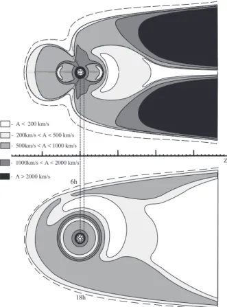
Fig. 1.A sketch of Alfv´en velocity distribution in the meridional(a)
and equatorial(b)sections of the magnetosphere. Areas with dif-ferent values ofAare shown by varying shades of grey. The NEPS in Fig. 1b has asymmetry due to convective flow of the plasma. An extensive area with a small value ofAon the right side of the fig-ure is a section of the plasma sheet in the distant tail. If it deviates from the equatorial plane, this area will be replaced by an area with a greater value ofA, corresponding to one of the tail lobes.
a moderately disturbed dayside magnetosphere. The fre-quencies of the eigenmodes are shown to be in the region f≥5 mHz. This result is easily understood from simple es-timates. In order of magnitude, the frequency of magne-tosonic oscillations equalsf∼A/λ, whereAis the typical Alfv´en velocity, λ is the wavelength. For an eigen-mode λ&L, whereLis the typical size of the resonator (if the res-onator’s sizes differ considerably in the different directions, Lis the smallest of them). For the head part of the magne-tosphere we haveA∼103km/s,L∼20RE∼105km, whence f∼A/L∼10 mHz, in complete agreement with the results of more precise calculations. One can see that the theoretical values for the frequencies differ too much from the observed ones. But there is an even more important reason not to allow the above-cited works to be regarded as acceptable versions of the global magnetospheric resonator. They ignore the ex-istence of the magnetospheric tail, and therefore the question of whether the eigenmodes are at all confined in the head part of the magnetosphere remains unanswered.
This question has brought to life a series of papers (Har-rold and Samson, 1992; Samson and Har(Har-rold, 1992; Sam-son and Rankin, 1994) treating the magnetospheric tail as the region where magnetosonic oscillations with a discrete spectrum are localised. In the meantime, the tail, due to its geometry, is not regarded as a resonator but rather as a waveguide along which generated oscillations can propa-gate freely. Frequency quantisation in such a waveguide is thought by the above authors to be provided for by the os-cillation having the structure of a standing wave along direc-tions transverse to the waveguide, with its wavelength along the waveguide being much larger than across, thereby not af-fecting the oscillation frequency. The latter suggestion seems too artificial, however. No reasons are apparent as to why the oscillations with a longitudinal wavelength on the order of the transverse wavelength or less cannot be excited. The spectrum of such oscillations is, in the meantime, continuous because the longitudinal wavelength can have any value (is not quantised) and affects the frequency considerably. This difficulty is recognised by the theory’s authors (Samson and Rankin, 1994) themselves. Besides, the theoretical oscilla-tion frequency considerably exceeds the observed one in this case as well. Lateral boundaries of such a waveguide are formed by the magnetopause (a 10 to 100-times Alfv´en ve-locity increase in it does produce the effect of reflection of magnetosonic waves). The typical value of the parameter L∼(2−3)·105km, and the typical value of the Alfv´en veloc-ity in the tail lobes (occupying most of its volume) mean-while isA∼(2−3)·103km/s, yieldingf ∼> 10 mHz.
Another version of the model in question exists where the waveguide is located in the plasma sheet (Siscoe, 1969). But this case also presents the same difficulties with explaining the discrete spectrum and the numerical value of the fre-quency. In the plasma sheet the typical value of the Alfv´en velocity isA∼102km/s, while its thickness isL∼2·104km, yieldingf∼5 mHz. Besides, due to the plasma in the plasma sheet being hot, the typical value of the frequency increases even more, being determined not only by the Alfv´en ve-locity but by the sound veve-locity in the plasmas as well: f∼√A2+S2/L.
is the case at the magnetopause. The reflection is not com-plete, with part of the wave’s energy penetrating into the so-lar wind. The portion of the wave’s energy passing through the magnetopause is proportional to the ratio of the Alfv´en velocities on both sides of the boundary.
Figure 1 shows sketches of the Alfv´en velocity isolines in the meridional and equatorial sections of the magnetosphere. They provide a complete enough representation of the three-dimensional distribution ofA. These figures rely on well-known data concerning the shape, sizes, magnetic field and density of plasma in the major structural components of the magnetosphere – the magnetopause, plasmasphere, external magnetosphere, plasma sheet, tail lobes (see, for example, Sergeev and Tsyganenko, 1980). These figures do not reflect many of the small-scale details in the distribution ofA, but we assume them to correctly describe its global distribution. In terms of the problem we are now discussing, the most important constituent in Fig. 1 is the large-scale and deep minimum ofA in the near-Earth part of the plasma sheet (NEPS). Figure 1 shows beyond a doubt that it is in this area that the possible existence of a resonator for global-scale magnetosonic waves should be investigated first. Such inspection at a qualitative-analysis level has recently been done by the authors (Leonovich and Mazur, 2005). Note that Fig. 1 exhibits two more areas with rather small val-ues ofA. The first one is the magnetopause-adjacent outer part of the dayside magnetosphere. It has modes localised in this area which were studied in Zhu and Kivelson (1989); Lee and Lysak (1991, 1994); Leonovich and Mazur (2001). As was mentioned above,f >10 mHz in this area. It is pos-sible that this resonator adjoins the resonator in the NEPS, thus forming its comparatively small-scale portion. This por-tion’s eigenmodes are part of the upper harmonics of the res-onator in the NEPS with quantum numbersn>5−10. Mean-while, it should be realised that the bulk of such a mode with n>5−10, specifically the bulk of its energy, lies in the NEPS. Secondly, a torus-shaped area with minimum Alfv´en ve-locity is located in the equatorial part of the plasmasphere. This area was first pointed out in Gul’elmi (1970) as a “ring trap for low-frequency waves in the Earth’s magnetosphere”. Estimates show thatf ∼>50 mHz in this area.
In this paper we theoretically investigate the structure and spectrum of some first harmonics of magnetosonic eigen-oscillations in the NEPS. We used a model of Alfv´en velocity distribution which, on the one hand, conveys the basic fea-tures of the distribution in Fig. 1, while, on the other hand, allows the variables in the oscillation equation to be sepa-rated. For this purpose, a parabolic system of coordinates is used where the magnetopause is represented as a paraboloid of rotation. It allows a far enough advance in the analytical solution of the problem, coming to numerical calculations at the final, rather simple, stage.
z r ϕ
Fig. 2. Model of the medium, and the coordinate system. The plasma sheet is grey. The near-Earth part of the plasma sheet (NEPS) has asymmetry about the z axis. Magnetopause is a paraboloid with its focus in the Earth’s centre. Coordinates (r, z, ϕ) form a cylindrical coordinate system.
Section 2 presents a distribution of the Alfv´en velocity value in the magnetotail as constructed based on satellite data. Based on these experimental data, an analytical, two-dimensional, inhomogeneous model of the magnetospheric plasma distribution is proposed in Sect. 3, which allows one to take into account the main regularities of the Alfv´en ve-locity distribution which are important for the problem un-der consiun-deration. The basic equations describing the spa-tial structure and spectrum of magnetosonic oscillations lo-calised in the NEPS are derived. In Sect. 4, the boundary conditions are obtained and the frequency spectrum of the basic harmonics of these oscillations is numerically calcu-lated. In Sect. 5, the calculated spectra are compared to frequencies of ULF oscillations, with discrete spectrum ob-served in the magnetosphere. Some features of the obob-served oscillations are discussed in terms of their being interpreted as the resonator eigenmodes in the NEPS. The Conclusion summarises the basic results of this work.
2 Model of the medium
The main structural elements of the magnetosphere nec-essary for our investigation are presented qualitatively in Fig. 2: the magnetospheric boundary (magnetopause) and the plasma sheet, dividing the magnetotail into two lobes. In the near-Earth part of the magnetosphere, the plasma sheet becomes significantly wider, occupying most of the magne-tospheric cavity. This is an important feature from the view-point of this research.
Note that the velocity distribution of magnetosonic waves in the magnetosphere is of fundamental importance for the problem under study. Velocity of fast magnetosonic waves is represented, in a certain approximation, byCf=
√ A2+S2,
whereA=B0/√4πρis the Alfv´en velocity, andS=√γ P /ρ
]5H
$NPV
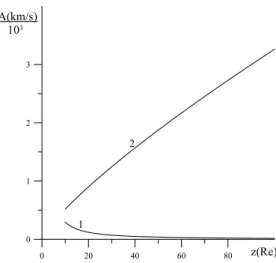
Fig. 3.Average statistical distribution of the Alfv´en velocity in the plasma sheet (1) and in the magnetotail lobes (2) in the tailward direction. The distributions are plotted using the approximation formulas in Sergeev and Tsyganenko (1980) for satellite-registered plasma concentration and geomagnetic field intensity. The origin z=0 is chosen at the Earth’s centre.
the distribution of sound velocity in the magnetosphere is much less known. This is due to sound velocity being a function of temperature, whose distribution in the magneto-sphere has been studied much less than the distribution of the magnetic field and plasma density. SinceS2/A2≈β, where β=8π P /B2is the gas-kinetic to magnetic pressure ratio, the distribution of the quantityβ in the magnetosphere may be examined.
In most of the magnetosphereβ≪1, because the magne-tosphere is actually a magnetic cavity in the solar wind flow, filled mainly with cold rare plasma. The magnetosphere has two areas where plasma density is comparatively high – the plasmasphere and the plasma sheet. But the plasmaspheric plasma is cold, while the geomagnetic field intensity is high, thereforeβ≪1 there, as well.
The situation in the plasma sheet is different. Plasma is hot here, whereas the magnetic field intensity is much lower than in the plasmasphere, therefore large values ofβ, including β≫1, are possible (Tsyganenko and Mukai, 2003). Due to the importance of this problem, we shall consider it in more detail.
To clearly understand the situation it is necessary to dis-tinguish between the two substantially different parts of the plasma sheet - NEPS and the distant plasma sheet (DPS). Both these parts are filled with nearly the same plasma in terms of density and temperature, so that the pressure in both is approximately the same, as well:PN EP S∼PDP S. Magne-tospheric convection causes this plasma to move from DPS to NEPS, where it precipitates into the ionosphere on the in-ner edge of the plasma sheet. In the process, diffuse aurorae are observed under quiet conditions, with auroral arcs and other active shapes observed under perturbed conditions. But
the geomagnetic field configuration in these two parts of the plasma sheet is completely different.
DPS can be regarded as an approximately flat sheet with the magnetic field changing its sign while varying from the value −BT in the tail’s one lobe up to BT in the other. Near the central plane of the DPS the magnetic field re-duces almost to zero. The equilibrium condition for DPS is PDP S=BT2/8π. It means that plasma pressure in the plasma sheet is balanced by magnetic pressure in the tail lobes. To compute the value ofβ near the central plane of the plasma sheet, one should keep in mind that the magnetic field actu-ally never turns into zero, due to the presence of a compara-tively small vertical componentBnin the field. The presence of this component results in the plasma sheet magnetic field lines being closed, even though they are very much tailward-elongated. On the order of magnitudeBn
>
∼0.1BT. Hence, βDP S=8π PDP S/Bn2 is obtained close to the central plane, which is completely with consistent the data in Tsyganenko and Mukai (2003).
The NEPS magnetic field is dipole-like and is strong enough in the entire region, at leastBN EP S&BT. Given that PN EP S∼PDP S, we haveβN EP S&1. The valuesβN EP S≫1 are impossible. They would mean the existence of plasma in the NEPS whose pressure could not be balanced. The NEPS dimensions, as well as those of the entire magneto-sphere, depend more on a magnetic disturbance level. Under quiet conditions, when KP=1−2, the NEPS inner edge is approximately 10RE, while its external edge is 20–30RE away. When the disturbance is large enough,KP
>
∼5, these distances decrease to, respectively, 5RE and 10RE. The ultra-low-frequency oscillations in which we are interested in are observed only when the disturbance is small,KP<3. Therefore, we shall tentatively assume the typical size of the NEPS under these conditions to be∼15RE=105km. The value βN EP S&1 denotes that S&A and Cf∼A in this re-gion. Therefore, all qualitative and, on the order of mag-nitude, quantitative conclusions are possible, if one assumes the plasma to be cold:Cf=A.
In the plasma sheet, the plasma density is significantly higher, and the Alfv´en velocity, respectively, is lower than in the magnetotail lobes. The boundary of the plasma sheet shown in Fig. 2 should be regarded as the boundary dividing the magnetospheric regions, resulting in large and small val-ues of the Alfv´en velocity. Therefore this boundary does not reach Earth, near which both geomagnetic field intensity and Alfv´en velocity increase.
are used for the plasma sheet, and B≈75/√z (nT) and n≈(10/z)2.6cm−3 for the magnetotail lobes, where the z
value is expressed in units of the Earth’s radius. In this case,A(km/s)≈2.18B(nT)/pn(cm−3)is the Alfv´en
veloc-ity. The maximum value of the Alfv´en velocity, about 5000 km/s, is reached in the lobes of the middle part of the magnetotail. Outside the magnetosphere the Alfv´en veloc-ity tends to 50–100 km/s, a value corresponding to the solar wind.
The Alfv´en velocity in the magnetotail lobes is more than an order of magnitude higher than in the plasma sheet. As will be shown below, it creates conditions for low-frequency magnetosonic waves to be confined in the NEPS. More de-tailed satellite measurements of the geomagnetic field inten-sity and plasma deninten-sity in the NEPS are presented in Borov-sky et al. (1998). Using these data we can determine the following typical values of the Alfv´en velocity:A≈240 km/s at a tailward distance from Earth z= −10RE, A≈70 km/s whenz= −15REandA≈200 km/s whenz= −25RE. Thus, we will assume that the typical value of the Alfv´en velocity in the NEPS is close to 200km/s.
3 Coordinate system and main equations
The spatial structure of the monochromatic fast magne-tosonic waves of the type ∼exp(−iωt ), where ω is the wave frequency, is described, in an inhomogeneous magne-tosphere, in the cold plasma approximation, by the equation
18+ω
2
A28=0, (1)
where8is any disturbed wave component of the oscillations under study,Ais the Alfv´en velocity. This equation should be treated as a model. Obtaining an accurate equation for the magnetosonic waves in a 3-D inhomogeneous magneto-sphere is rather problematic. Its form depends on both the method of dividing the entire field of MHD oscillations into constituent fields of the Alfv´en and magnetosonic waves, as well as on the chosen coordinate system. The coefficients for the derivatives are, of course, different in various curvilinear coordinate systems. When the typical spatial scales of the os-cillations under study are much smaller than the typical scale of changes in the medium parameters, however, Eq. (1) de-scribes, with good accuracy, the structure of a magnetosonic wave in any orthogonal coordinate system. At the limit of its applicability, this equation can also be used for oscillations whose wavelength is comparable with the typical scales of the medium inhomogeneity.
The search for a solution to Eq. (1) is significantly simpli-fied if symmetry in some direction is present in the problem. We, in our work, will be interested in the magnetosonic os-cillations localised in the NEPS. As follows from Fig. 2, in this part of the magnetosphere there is some axial (about the zaxis) symmetry. Plasma sheet geometry in the middle and
distant tail breaks this symmetry, of course. But for the prob-lem we discuss, the presence of the distant plasma sheet is inessential, and we can totally neglect it. Both the tail lobes and the distant plasma sheet are opacity regions for the oscil-lations under examination. Indeed, as follows from Eq. (1), the local dispersion equationω2=(k2x+ky2+kz2)A2(x, y, z)– wherekx,y,z=2π/λx,y,z are the local wave numbers,λx,y,z are the local wavelengths on the coordinates(x, y, z)– holds in the WKB approximation for the magnetosonic waves. The valueA¯≈200 km/s is typical of the NEPS, and for the fun-damental harmonics we haveλx,y,z≥105km (typical wave-lengths along all the directions are approximately the same). Thus, for the frequency of fundamental harmonics we have f=ω/2π≈A/λ≈0.5 mHz. Expressing the squared wave number on thezaxis from the local dispersion equation, we obtain
k2z(x, y, z)= ω
2
A2 −(k 2
x+ky2).
Suppose that there is a transparency region in the NEPS for the low-frequency waves under study. It means that here, ω2/A2∼>k2x+ky2. Moving to the tail lobes the Alfv´en veloc-ity increases by an order of magnitude, but the wave numbers k2x, ky2, the value of which is determined by the typical scale of the localisation region (in our case, by the typical radius of the geotail cross section), remain practically unchanged. The eventual result is that we havekz2<0 in the tail lobes and, thus, they become an opacity region for the low-frequency magnetosonic waves under consideration. It allows us to use an axisymmetric model of the magnetosphere and to translate the initial three-dimensional inhomogeneous problem into a two-dimensional one, which is much simpler for investiga-tion.
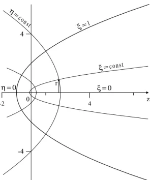
Since the magnetospheric cavity resembles a paraboloid, it is natural to choose the parabolic coordinate system to de-scribe it (Madelung, 1961). We will introduce two mutu-ally orthogonal sets of parabolic coordinate surfaces having a common focus at the centre of Earth, denoting them asξ andη. These surfaces are obtained by rotating the genera-trix parabolas about thezaxis, thereby passing through the centres of the Sun and Earth (see Fig. 4). The dimensionless parabolic coordinatesξ andηare related to the usual cylin-drical coordinates (thezaxis being common) by
ξ =(pr2+z2−z)/2σ,
η=(pr2
+z2
+z)/2σ,
whereσ is the distance from the focus to the top of the pa-raboloidξ=1, corresponding to the magnetopause. In other words,σ is the distance from the Earth’s centre to the sub-solar magnetopause point. Since we assume axial symme-try in the problem, we will seek its full solution as an ex-pansion into azimuthal harmonics of the type8(ξ, η, ϕ) =
¯
]
ξ = c o n st η = con
st ξ = 1
ξ = 0 η = 0
U
Fig. 4. An orthogonal system of dimensionless parabolic coordi-nates (ξ, η) in a cross section containing thezaxis. The focusz=0 is located at the Earth’s centre. The surfaceξ=1 coincides with the magnetopause. Semiaxesz=(0,∞)andz=(0,−∞)coincide with the coordinate surfacesξ=0 andη=0, respectively.
number. Equation (1) written in the parabolic coordinatesξ andηhas the form
∂ ∂ξξ
∂8¯ ∂ξ +
∂ ∂ηη
∂8¯
∂η (2)
+
"
(ξ+η) ω
2σ2
A2(ξ, η)−
m2 4
1 ξ +
1 η
#
¯ 8=0. It is easy to verify that if we choose the Alfv´en velocity dis-tribution as
A2(ξ, η)= A
2 0
σ
ξ+η a(ξ )+b(η),
whereA0is a constant with the dimension of velocity, and
a(ξ ) andb(η) are any functions of the variables ξ andη, then Eq. (2) becomes an equation with separable variables.
Such functionsa(ξ )andb(η)have to be chosen as to al-low us to simulate the chief regularities of the Alfv´en veloc-ity distribution in the magnetospheric region of interest. We will consider the oscillations localised in the magnetosphere, neglecting their small leakage into the solar wind through the magnetopause. Therefore, we will not require correct be-haviour from the functionA2(ξ, η)in the solar wind region when choosing the functionsa(ξ )andb(η). The major reg-ularities of the Alfv´en velocity distribution in the NEPS and in the magnetotail lobes can be modelled by the following functions
a(ξ )= [α0+(α1−α0)ξ]ξ, (3)
b(η)=
[α0+(α2−α0)η]η, η≤η1,
β1[1−(η−ηmin)2/121], η1< η < η2,
β2[1+(η−ηmax)2/122], η≥η2,
(4)
whereηminis the coordinate corresponding to the location of
an Alfv´en velocity minimum in the NEPS, andηmax is the
coordinate of a maximum in the middle part of the magne-totail lobes. Parameters of the model (4) are assumed to be chosen such that the functionb(η)is continuous and smooth. The pointsη1andη2can be conventionally considered as the
near and far (relative to Earth) boundaries of the NEPS on theηcoordinate. It is between these points that the turning points of oscillations localised in the NEPS are to be found. The maximum of the Alfv´en velocity value in the middle part of the magnetotail serves as a potential barrier for confining low-frequency magnetosonic oscillations in the NEPS. For higher-frequency oscillations this maximum is not a barrier in preventing their tailward escape. This is probably why higher-frequency MHD oscillations with discrete spectrum are not observed in the magnetosphere.
Thus, if the wave function under investigation is presented as8(ξ, η)¯ =ψ (ξ )φ (η), we can reduce the search for a solu-tion to the initial partial of the differential equasolu-tion to solving a system of two coupled ordinary differential equations:
ξ∂
2ψ
∂ξ2 +
∂ψ ∂ξ +
"
2a(ξ )−m
2
4ξ +Q
#
ψ=0, (5)
η∂
2φ
∂η2 +
∂φ ∂η +
"
2b(η)−m
2
4η −Q
#
φ=0. (6)
HereQis the separation constant, and=ωσ/A0is the
di-mensionless frequency. These quantities are the eigenvalues of the problem to be solved.
4 Results of numerical calculations and their discussion
Numerically computing the eigenfrequency spectrum of os-cillations localised in the NEPS requires constants which de-termine the parameters of the magnetospheric model to be specified, Eqs. (3), (4). Let us choose the following nu-merical values for the constants: A0=750 km/s, σ=10RE (RE=6370 km is the Earth’s radius),α0=0.04,α1=10,α2=5,
ηmin=1.5,ηmax=6,11=1,12=2.5,η1=0.6, and the η2 point
is found based on the requirement that the second and third expressions in Eq. (4) are equal whenη=η2. The
appropri-ate two-dimensional (in a meridional plane) distribution of the Alfv´en velocity is shown in Fig. 5. This model describes well enough both the distribution of the Alfv´en velocity in the NEPS (η1<η<η2) and its maximum in the middle tail, as
well as demonstrating a qualitatively correct behaviour in the earthward direction.
]
[
Fig. 5. Isolines of Alfv´en velocity valueA(103km/s) distribution used in the model calculations, in the plane (x, z). Coordinatesx andzare in units ofσ – distance from the Earth’s centre to the subsolar point of the magnetopause. The localisation of the NEPS region is 0.6<z<2.5. The region of the Alfv´en velocity maximum in the magnetotail lobes isz≈6.5.
the small leakage of the oscillations in question into the solar wind, an external boundary condition for the functionψ (ξ ) can be formulated at the magnetopause, whereξ=1. Let us consider this boundary to be an ideally reflecting wall, which gives us the first boundary conditionψ (1)=0. The second boundary condition will be imposed on the symmetry axis: ξ = 0. As ξ→0, the first term in the square brackets in Eq. (5) can be neglected, and the remaining equation reduces to a Bessel equation solved by the Bessel functions:
ψ (ξ )=CJ2m(2
p
Qξ )+DY2m(2
p
Qξ ),
whereC andDare arbitrary constants. We will require that the solution be finite in its entire domain. Since the function Yν(x)has a singularity asx→0, we will assumeD=0.
A similar boundary condition is obtained for the function φ (η)asη→0:
φ (η)=CI2m(2
p
Qη).
For the oscillations we are discussing, there are turning points,η¯1andη¯2(0<η¯1<η¯2<η2), in the WKB
approxima-tion, between which they are localised. When η>η¯2, the
functionφ (η)decreases exponentially in the opacity region. Moving further away tailwards, the Alfv´en velocity, having passed its maximum, begins to decrease, and the opacity re-gion is followed again by the transparency rere-gion. This cre-ates conditions for the oscillations to partially leak through the potential barrier into the solar wind.
However, if this barrier is wide and high enough, oscil-lation leakage through it is small (smaller than through the magnetopause), and can be neglected. Thus, the second boundary condition can be formulated in this approximation as an impenetrable wall located deep in the opacity region. If it is located much farther than the typical scale of the function φ (η)’s exponential decay into the opacity region, the solution to be obtained is practically unaffected by where in particu-lar, this wall is located. We, in our calculations, placed it in the region of the Alfv´en velocity maximum:φ (ηmax)=0.
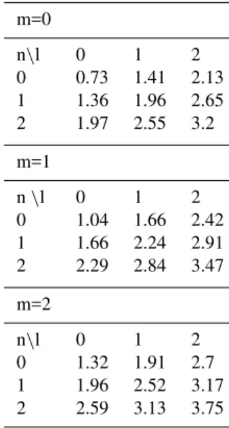
Table 1. Eigenfrequencies of the MHD resonator in the NEPS – fmnl(mHz).
m=0
n\l 0 1 2
0 0.73 1.41 2.13
1 1.36 1.96 2.65
2 1.97 2.55 3.2
m=1
n\l 0 1 2
0 1.04 1.66 2.42
1 1.66 2.24 2.91
2 2.29 2.84 3.47
m=2
n\l 0 1 2
0 1.32 1.91 2.7
1 1.96 2.52 3.17
2 2.59 3.13 3.75
These boundary conditions are only satisfied by solutions of Eqs. (5), (6) corresponding to certain eigenvalues of the parameters=mnlandQ=Qmnl, wherem, n, l=0,1,2. . . – i.e. quantum numbers determining the number of nodes of the desired localised wave function8mnl(ϕ, ξ, η)on the coordinates ϕ, ξ and η, respectively. The set of eigen-values mnl determines the set of resonator eigenfrequen-cies fmnl=ωmnl/2π. The first three harmonics’ eigenfre-quencies, for all quantum numbers, found while numeri-cally solving the problem, are presented in Table 1. One can see that the calculated eigenfrequencies tally rather well with the observed frequency spectrum of the magne-tospheric low-frequency oscillations with discrete spectrum (0.8, 1.3, 1.9, 2.6 ... mHz). There is one interesting fea-ture observed in the spectrum of the calculated frequen-cies. The resonator eigenfrequencies do not cover the spec-trum range evenly, but converge into separate groups. Thus, the frequencies f000=0.73 mHz and f100=1.04 mHz
repre-sent groups consisting of a single frequency. Each of the frequency groups (f001=1.41; f010=1.36; f200=1.32 mHz)
and (f101=1.66; f110=1.66; f300=1.59 mHz) include
Other conditions being equal, the ratio between the num-ber of harmonics in the groups can be regarded as a relative probability of observing oscillations with the given average frequency. It is difficult, however, to imagine that the excita-tion condiexcita-tions can be the same for oscillaexcita-tions with different spatial structures. This probability is primarily influenced by the presence of a harmonic of given oscillations in the source spectrum. As a source of these oscillations, one could regard, for example, the Kelvin-Helmholtz instability at the magne-topause. The eigenfrequency spectrum of the resonator in question is precisely within the frequency range of oscilla-tions excited by this instability in the magnetotail (Sibeck et al., 1987). These oscillations can also be excited in the mag-netosphere under the effect of solar wind pressure impulses (Kepko and Spence, 2003).
5 Discussion
Let us discuss some features of ULF oscillations with a dis-crete frequency spectrum registered in the magnetosphere, regarding them as the eigenmodes of a resonator in the NEPS. Observations imply that these oscillations are chiefly registered in the magnetosphere’s midnight-morning sector. The NEPS is known to have noticeable asymmetry rela-tive to the midnight-afternoon meridional plane (Elpic et al., 1999). This is related to the asymmetry of the convective plasma flux from the magnetotail to the dayside, more in-tense through the morning than through the evening sector of the magnetosphere. The bulk of the NEPS meanwhile shifts into the morning sector and its projection along the field lines onto Earth occupies latitudes between 60◦–80◦. Owing to the
eigen-oscillations localised in this part of the plasma sheet, their absence from the dayside and evening magnetosphere receives a natural explanation.
Unfortunately, there is no similar natural and exhaustive explanation for the stability of the registered oscillations’ fre-quencies. Magnetospheric parameters vary within very wide limits, depending on the degree to which the geomagnetic field is disturbed. This is a common difficulty for any ex-isting theoretical interpretations of the observed oscillations. It is possible, however, to try to understand this feature by way of the following reasoning. For an eigen oscillation to set in the resonator, its parameters should remain unchanged for at least several oscillation periods. Since the oscillations in question are sufficiently low-frequency (with periods of about 20 min), we can assume that the resonator character-istics remain constant for an hour or more. This is possible only in quiet enough periods in terms of geomagnetic dis-turbances. As follows from observations, low-frequency os-cillations with discrete spectrum are indeed most often reg-istered on a quiet enough geomagnetic background (Mathie et al., 1999). The plasma sheet (at least the NEPS), in the meantime, has probably almost the same parameters, which is what determines the stability of registered frequencies.
When the level of geomagnetic activity rises the plasma sheet characteristics (as well as those of the confining barrier in the tail lobes) lose their stability, and the eigenmodes have suf-ficient time to form and stand out against a background of changing magnetospheric parameters.
One more observation concerns the oscillations registered on the Earth’s surface. It is presumed that the Alfv´en waves registered on Earth have been generated on the resonant mag-netic shells via the mechanism of field line resonance. The internal part of the magnetosphere adjoining the Earth is an opacity region for the magnetosonic waves under considera-tion and their amplitude decreases exponentially earthwards (Mathie et al., 1999; Leonovich and Mazur, 2001; Wanliss et al., 2002). Thus, it seems that these oscillations cannot be registered on the Earth’s surface proper.
These ideas, however, are only applicable for oscillations with wavelengths that are much smaller than the typical in-homogeneity scales of the magnetospheric plasma. The low-frequency magnetosonic oscillations we are now discussing have a typical variation scale comparable with the typical scales of magnetospheric inhomogeneity. Therefore, such large-scale magnetosonic oscillations can reach Earth with-out their amplitude having dropped significantly. On the whole, the issue of the oscillations under study penetrating to the Earth’s surface requires further research, including their ground-level polarization.
6 Conclusions
The main results of this work may be summarised as follows: 1. A new concept is proposed for low-frequency oscilla-tions with discrete spectrum which are registered by HF radars and networks of ground-based magnetome-ters at high latitudes. The quantisation of oscillation fre-quencies is supposed to be related to their being eigen-modes of the resonator in the near-Earth plasma sheet (NEPS). A small value of the Alfv´en velocity in the NEPS determines the low frequency of the resonator eigen-oscillations. The confinement of the oscillations within the resonator is provided for by the presence of a potential barrier related to the maximum in the distri-bution of the Alfv´en velocity over the middle part of the magnetotail lobes.
2. A resonator frequency spectrum was computed for the NEPS. A model magnetosphere with parabolic geom-etry was used. A two-dimensional inhomogeneous model of the Alfv´en velocity distribution was proposed for the calculations, which takes into account both the minimum in the NEPS and the maximum in the lobes of the mid magnetotail, confining the oscillations in the tailward direction. The eigenfrequencies of such a res-onator are shown to form separate groups, whose aver-age frequencies (f¯≈0.73, 1.04, 1.35, 1.6, 1.95, 2.2, 2.6, 3.1 . . . mHz) are close to the frequencies of ob-served oscillations with discrete spectrum (0.8, 1.3, 1.9, 2.6 . . . mHz).
3. Asymmetry in the occurrence of oscillation registration between the midnight-morning and midnight-evening magnetospheric sectors is explained by the asymmetry of the NEPS.
Acknowledgements. This work was partially supported by Russian Foundation for Basic Research grants: RFBR 04-05-64321 and RFBR 06-05-64495, Program of presidium of Russian Academy of Sciences #16 and OFN RAS #16.
Topical Editor I. A. Daglis thanks two referees for their help in evaluating this paper.
References
Borovsky, J. E., Thomsen, M. F., Elphic, R. C., Cayton,T. E., and McComac, D. J.: The transport of plasma sheet material from the distant tail to geosynchronous orbit, J. Geophys. Res., 103, 20 297–20 331, 1998.
Dungey, J. W.: Electrodynamics of the outer atmospheres, Ionos. Sci. Rep., 69, Ionos. Res. Lab., Cambridge, Pa., 1954.
Elphic, R. C., Thomsen, M. F., Borovsky, J. E., and McComas,D. J.: Inner edge of the electron plasma sheet: empirical models of boundary location, J. Geophys. Res., 104, 22 679–22 693, 1999. Gul’elmi, A. V.: The ring trap for low-frequency waves in the
Earth’s magnetosphere (in Russian), Pis’ma Zh. Eksp. Teor. Fiz., 12, 35–38, 1970.
Harrold, B. G. and Samson, J. C.: Standing ULF modes of the mag-netosphere: a theory, Geophys. Res. Let., 19, 1811–1814, 1992. Kepko, L. and Spence, H. E.: Observation of discrete,
global magnetospheric oscillations directly driven by so-lar wind density variations, J. Geophys. Res., 108, 1257, doi:1029/2002JA009676, 2003.
Kivelson, M. G. and Southwood, D. J.: Resonant ULF waves: a new interpretation, Geophys. Res. Let., 12, 49–52, 1985. Kivelson, M. G. and Southwood, D. J.: Coupling of global
magne-tospheric MHD eigenmodes to field line resonances, J. Geophys. Res., 91, 4345–4351, 1986.
Lee, D.-H. and Lysak, R. L.: Monochromatic ULF wave excita-tion coupling in the dipole magnetosphere, J. Geophys. Res., 96, 5811–5823, 1991.
Lee, D.-H. and Lysak, R. L.: Numerical studies on ULF wave struc-tures in the dipole model, in: Solar Wind Sources of Magne-tospheric Ultra-Low-Frequency Waves, Geophys. Monogr. Ser., vol. 81, edited by: Engebretson, M., Takahashi, J. K., and Sc-holer, M., AGU, Washington, D.C., 293–297, 1994.
Leonovich, A. S. and Mazur, V. A.: Resonance excitation of standing Alfven waves in an axisymmetric magnetosphere (monochromatic oscillations), Planet. Space Sci., 37, 1095– 1108, 1989.
Leonovich, A. S. and Mazur, V. A.: On the spectrum of magne-tosonic eigenoscillations of an axisymmetric magnetosphere, J. Geophys. Res., 106, 3919–3928, 2001.
Leonovich, A. S. and Mazur, V. A.: Why do ultra-low-frequency MHD oscillations with a discrete spectrum exist in the magneto-sphere?, Ann. Geophys., 23, 1075–1079, 2005.
Lessard, M. R., Hanna, J., Donovan, E. F., and Reeves, G. D.: Evidence for a discrete spectrum of persistent magnetospheric fluctuations below 1 mHz, J. Geophys. Res., 108(A3), 1125, doi:10.1029/2002JA009311, 2003.
Madelung, E.: Mathematical tools for the physicist, (in Russian), Nauka, Moscow, 275–276, 1961.
Mann, I. R., Wright, A. W., Mills, K. J., and Nakariakov, V. M.: Ex-citation of magnetospheric waveguide modes by magnetosheath flows, J. Geophys. Res., 104(A1), 333–354, 1999.
Mathie, R. A., Menk, F. W., Mann, I. R., and Orr, D.: Discrete field line resonances and the Alfven continuum in the outer magneto-sphere, Geophys. Res. Lett., 26, 659–662, 1999.
McClay, J. F.: On resonant modes of a cavity and the dynamical properties of micropulsations, Planet. Space Sci., 18, 1673–1682, 1970.
Ruohoniemi, J. M., Greenwald, R. A., and Baker, K. B.: HF radar observations of Pc5 field line resonances in the midnight/early morning MLT sector, J. Geophys. Res., 96, 15 697–15 710, 1991. Samson, J. C. and Harrold, B. G.: Field line resonances associated with waveguides in the magnetosphere, Geophys. Res. Lett., 19, 441–444, 1992.
Samson, J. C., and Rankin, R.: The coupling of solar wind energy to MHD cavity modes, waveguide modes and field line resonances in the Earth’s magnetosphere, in: Solar Wind Sources of Magne-tospheric Ultra-Low-Frequency Waves, Geophys. Monogr. Ser., vol. 81, edited by: Engebretson, M. J., Takahashi, J. K., and Sc-holer, M., 253–264, AGU, Washington, D.C., 1994.
Sergeev, V. A. and Tsyganenko, N. A.: The Earth’s magnetosphere (in Russian), Moscow, Nauka, 1980.
crossings – Evidence for the Kelvin-Helmholtz instability, in: Magnetotail physics (A88–46526 19–46), Baltimore, MD, Johns Hopkins University Press, 73–76, 1987.
Siscoe, G. L.: Resonant compressional waves in the geomagnetic tail, J. Geophys. Res., 74, 6482–6486, 1969.
Southwood, D. J. and Kivelson, M. G.: The effect of parallel inho-mogeneity of magnetospheric hydromagnetic wave coupling, J. Geophys. Res., 91, 6871–6877, 1986.
Tsyganenko, N. A. and Mukai, T.: Tail plasma sheet models de-rived from Geotail particle data, J. Geophys. Res., 108, 1136, doi:10.1029/2002JA009707, 2003.
Wanliss, J. A., Rankin, R., Samson, J. C., and Tikhonchuk, V. T.: Field line resonances in a stretched magnetotail: CANOPUS optical and magnetometer observations, J. Geophys. Res., 107, SMP9,1100, doi:10.1029/2001JA000257, 2002.