A statistical subgrid-scale algorithm for precipitation formation in stratiform clouds in the ECHAM5 single column model

(1)

ACPD

11, 9335–9374, 2011

Sub-column algorithm in ECHAM5-HAM

S. Jess et al.

Title Page

Abstract Introduction

Conclusions References

Tables Figures

◭ ◮

Back Close

Full Screen / Esc

Printer-friendly Version Interactive Discussion

Discussion

P

a

per

|

Dis

cussion

P

a

per

|

Discussion

P

a

per

|

Discussio

n

P

a

per

|

Atmos. Chem. Phys. Discuss., 11, 9335–9374, 2011 www.atmos-chem-phys-discuss.net/11/9335/2011/ doi:10.5194/acpd-11-9335-2011

Atmospheric Chemistry and Physics Discussions

This discussion paper is/has been under review for the journal Atmospheric Chemistry and Physics (ACP). Please refer to the corresponding final paper in ACP if available.

A statistical subgrid-scale algorithm for

precipitation formation in stratiform

clouds in the ECHAM5 single column

model

S. Jess1, P. Spichtinger1,*, and U. Lohmann1

1

ETH Zurich, Institute for Atmospheric and Climate Science, 8092 Zurich, Switzerland

*

now at: Institute for Atmospheric Physics, Johannes Gutenberg-University, Mainz, Germany Received: 12 November 2010 – Accepted: 18 February 2011 – Published: 22 March 2011 Correspondence to: S. Jess (stephanie.jess@env.ethz.ch)

(2)

ACPD

11, 9335–9374, 2011

S. Jess et al.

Title Page

Tables Figures

◭ ◮

Back Close

Full Screen / Esc

Discussion

P

a

per

|

Dis

cussion

P

a

per

|

Discussion

P

a

per

|

Discussio

n

P

a

per

|

Abstract

Cloud properties are usually assumed to be homogeneous within the cloudy part of the grid-box, i.e. subgrid-scale inhomogeneities in cloud cover and/or microphysical properties are often neglected. However, precipitation formation is initiated by large particles. Thus mean values are not representative and could lead to a delayed onset 5

of precipitation.

For a more physical description of the subgrid-scale structure of clouds we introduce a new statistical sub-column algorithm to study the impact of cloud inhomogeneities on stratiform precipitation. Each model column is divided intoN_{independent sub-columns}

with sub-boxes in each layer, which are completely clear or cloudy. The cloud cover 10

is distributed over the sub-columns depending on the diagnosed cloud fraction. Mass and number concentrations of cloud droplets and ice crystals are distributed randomly over the cloudy sub-columns according to prescribed probability distributions. Shapes and standard deviations of the distributions are obtained from aircraft observations.

We have implemented this sub-column algorithm into the ECHAM5 global climate 15

model to take subgrid variability of cloud cover and microphysical properties into ac-count. Simulations with the Single Column Model version of ECHAM5 were carried out for one period of the Mixed-Phase Polar Arctic Cloud Experiment (MPACE) campaign as well as for the Eastern Pacific Investigation of climate Processes (EPIC) campaign. Results with the new algorithm show an earlier onset of precipitation for the EPIC cam-20

(3)

ACPD

11, 9335–9374, 2011

S. Jess et al.

Title Page

Tables Figures

◭ ◮

Back Close

Full Screen / Esc

Discussion

P

a

per

|

Dis

cussion

P

a

per

|

Discussion

P

a

per

|

Discussio

n

P

a

per

|

1 Introduction

Clouds are one fundamental component of the climate system. They are important reg-ulators of the radiation budget (Kiehl and Trenberth, 1997) and the hydrological cycle (Chahine, 1992). The mean global cloud cover amounts to 60–70% (Raschke et al., 2005). Global climate models (GCM) that simulate the future climate are limited to 5

a coarse resolution on the order of 100 km horizontal grid space due to computational costs. One key issue for improving the representation of clouds in large-scale models is their inhomogeneity: GCMs use grid mean quantities of cloud properties to calculate cloud microphysical and macrophysical processes, i.e. they represent layers of clouds, which are homogeneous with respect to microphysical properties (e.g. mass and num-10

ber concentration of cloud droplets and ice crystals). In nature, however, clouds are inhomogeneous in terms of microphysical properties. Larson et al. (2001) stated that models using convex autoconversion functions like the ECHAM model to parameterize the precipitation formation underpredict autoconversion rates. The bias is corrected by tuning parameters, which artificially increase the amount of rain formed. Rotstayn 15

(2000) studied the impact of tuned autoconversion rates in climate models. He found that including some part of subgrid variability in liquid water content into the parameteri-zation of autoconversion of Manton and Cotton (1977) permits to increase the threshold radius above which autoconversion commences. This leads to a more physically based threshold than Rotstayn (2000) used before. Jakob and Klein (2000) showed that pa-20

rameterizations considering the cloud-precipitation overlap inside a grid-box can partly account for deficiencies in evaporation and accretion rates. Morrison and Gettelman (2008) considered subgrid variability of liquid water content in their cloud microphysics scheme. The largest sensitivity was found in the autoconversion rate due to its high nonlinearity.

25

(4)

ACPD

11, 9335–9374, 2011

S. Jess et al.

Title Page

Tables Figures

◭ ◮

Back Close

Full Screen / Esc

Discussion

P

a

per

|

Dis

cussion

P

a

per

|

Discussion

P

a

per

|

Discussio

n

P

a

per

|

a lower mean albedo than a horizontally homogeneous medium of the same optical thickness (Weinman and Swarztauber, 1968). The huge variability of the cloud struc-ture at different altitudes is partly responsible for the difficulty in representing clouds in GCMs correctly. It can cause errors in the development of microphysical properties like droplet and ice crystal growth and also number concentration because subgrid variabil-5

ity is not well represented. Mean values for cloud variables at each grid point neglect the natural variations and therefore important information will be lost. This shortcom-ing could lead to uncertainties regardshortcom-ing the equilibrium climate for a doublshortcom-ing of CO₂ (Tsushima et al., 2006). The precipitation formation in ECHAM5 is currently calculated using mean values of the cloud condensate in the cloudy part of the grid-box. However, 10

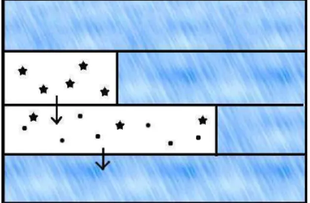
mean values in a grid-box are not representative for the formation of precipitation as all collection processes start with the large particles in the cloud and more than one cloud could occupy a grid cell of a GCM. Also the treatment of precipitation is not han-dled accurately in the present model configuration (Fig. 1a). One solution of a more accurate treatment is shown in Fig. 1b (details later).

15

The fluxes from above are able to interact with the entire cloudy part of the grid box in the level below in the present model configuration. For example the accretion of cloud droplets by rain is calculated for the whole cloudy part and is then weighted with the minimum of precipitation fraction and cloud cover. This leads to errors if the cloud cover in the level below is different from the cloud cover above because clouds are inhomoge-20

neous. If ice crystals sediment into a lower liquid cloud containing supercooled water droplets, the droplets may be converted into ice crystals by the Bergeron-Findeisen process (Baker, 1997). Therefore, it depends crucially on the vertical distribution of the cloud if ice crystals falling into the lower cloud initiate precipitation or sublimate in a cloud-free region.

25

There are different possibilities to include subgrid variability into a large scale model. Some of them are listed below.

(5)

ACPD

11, 9335–9374, 2011

S. Jess et al.

Title Page

Tables Figures

◭ ◮

Back Close

Full Screen / Esc

Discussion

P

a

per

|

Dis

cussion

P

a

per

|

Discussion

P

a

per

|

Discussio

n

P

a

per

|

subgrid-scale distribution of clouds can be derived within the framework of a statistical-dynamical approach, e.g., Tompkins (2002), where the probability density function (PDF) approach uses a beta distribution for the total water mixing ratio and predicts its shape parameters from processes such as deep convection, turbulence and microphysics.

5

2. The Monte Carlo Independent Column Approximation (McICA) (Barker et al., 2002) could be applied to compute domain-averaged, broadband radiative flux profiles. The calculation of the radiative fluxes is separated into the clear-sky and the cloudy part of the grid-box for which different possible cloud states could be assumed. For instance, each column of the model is divided into a number of 10

sub-columns (Pincus et al., 2003). The broadband fluxes are calculated sepa-rately by performing 1-D radiative transfer calculations on each sub-column and the domain-average fluxes are then obtained. R ¨ais ¨anen et al. (2004) used the sub-column approach explained above for the radiation scheme of the ECMWF model. Cloud properties are distributed with PDFs into the cloudy sub-boxes of 15

each layer to account for horizontal variability.

Another realization of this sub-column approach was used by Jakob and Klein (1999) in a subgrid-scale precipitation model, which resolves the vertical variation of cloud fraction. The subgrid model divides the grid-boxes into homogeneous columns with sub-boxes, which are either completely clear or cloudy. The mean 20

cloud condensate within the cloudy part of the entire grid box is used for each cloudy sub-box. In a next step the microphysical parameterization is calculated separately and independently for each column of sub-boxes.

3. The superparameterization of Grabowski (2001) is a possibility to couple small-scale processes with the large-small-scale dynamics. Here a two-dimensional cloud 25

(6)

ACPD

11, 9335–9374, 2011

S. Jess et al.

Title Page

Tables Figures

◭ ◮

Back Close

Full Screen / Esc

Discussion

P

a

per

|

Dis

cussion

P

a

per

|

Discussion

P

a

per

|

Discussio

n

P

a

per

|

scheme permits to simulate e.g. deep convection, fractional cloudiness and cloud overlap explicitly, however with high computational demand.

In this study, the cloud generator as introduced by Jakob and Klein (1999) and R ¨ais ¨anen et al. (2004) is used to capture some of the unresolved subgrid variability of clouds in the ECHAM5 GCM with emphasis on precipitation formation.

5

Jakob and Klein (1999) show that the subgrid model calculates less evaporation in the middle troposphere in the tropics resulting in more realistic simulations than without this treatment. The findings of R ¨ais ¨anen et al. (2004) indicate that biases in radiative fluxes and heating rates could be reduced by 25–50% as compared to studies with horizontally homogeneous clouds.

10

Compared to the superparameterization of Grabowski (2001), the algorithm used in this study to include subgrid variability is not deterministic but statistical and does not involve coupling to the dynamics, but primary addresses microphysical processes of stratiform clouds. The column algorithm has no time-dependency and the sub-columns representing one column of a GCM are horizontally independent. We intro-15

duce inhomogeneities in the microphysical properties of stratiform clouds, which then affect precipitation formation. Distributions of cloud properties are considered instead of averaged in-cloud values used by Jakob and Klein (1999).

The observations of the Eastern Pacific Investigation of Climate processes (EPIC) campaign (Bretherton et al., 2004) and the Mixed-Phase Polar Arctic Cloud Experi-20

ment (MPACE) campaign (Verlinde et al., 2007) are used to validate the Single Column Model (SCM) simulations.

Section 2 explains the model physics while Sect. 3 documents the algorithm. The results are displayed in Sect. 4 followed by the discussion of the results in Sect. 5. Sensitivity studies of the algorithm are described in Sect. 6 and finally conclusions are 25

(7)

ACPD

11, 9335–9374, 2011

S. Jess et al.

Title Page

Tables Figures

◭ ◮

Back Close

Full Screen / Esc

Discussion

P

a

per

|

Dis

cussion

P

a

per

|

Discussion

P

a

per

|

Discussio

n

P

a

per

|

2 Model description

We use the ECHAM5 GCM (Roeckner et al., 2003) to investigate the effects of hetero-geneous cloud properties on precipitation formation for stratiform clouds. The version of ECHAM5 used in this study is described in Lohmann et al. (2008). The stratiform cloud scheme uses prognostic equations for water vapor, liquid and ice, bulk cloud 5

microphysics (Lohmann and Roeckner, 1996) and a statistical cloud cover scheme (Tompkins, 2002). Phase changes between the water components and precipita-tion processes (autoconversion, accreprecipita-tion, aggregaprecipita-tion) are considered in the cloud scheme. It contains the evaporation of rain, melting and sublimation of snow and cloud ice as well as sedimentation of cloud ice. Prognostic equations of the number concen-10

trations of cloud droplets and ice crystals in stratiform clouds are used and ECHAM5 has been coupled to the aerosol scheme HAM (Stier et al., 2005). The autoconversion scheme of Khairoutdinov and Kogan (2000) was chosen for all simulations. Additionally for a consistent use of the sub-column algorithm, the sequence of cloud microphysical calculations is changed as compared to the original version. Condensation and depo-15

sition is calculated first in order to obtain the liquid and ice water content which can then be distributed over the cloudy sub-boxes in the sub-columns.

3 Sub-column algorithm for microphysics

The basic idea of the algorithm is the following: first, each grid box is divided into a number N _{of homogeneous and independent sub-columns (see Fig. 1b). Second,}

20

the number of cloudy sub-boxes in each layer is defined by the nearest integer of the product ofN sub-columns and the diagnosed cloud fraction in each layer. In this study a maximum-random overlap assumption for the vertical distribution of clouds is used following Jakob and Klein (1999). Third, the clouds are distributed depending on the overlap assumption. The sub-boxes are filled in a left to right order fullfilling the 25

(8)

ACPD

11, 9335–9374, 2011

S. Jess et al.

Title Page

Tables Figures

◭ ◮

Back Close

Full Screen / Esc

Discussion

P

a

per

|

Dis

cussion

P

a

per

|

Discussion

P

a

per

|

Discussio

n

P

a

per

|

water content (LWC), ice crystal number concentration (ICN) and cloud droplet number concentration (CDNC)) is allocated for the cloudy sub-boxes in a fourth step. We use a log-normal size distribution with prescribed standard deviations for IWC, LWC, ICNC and CDNC taken from atmospheric measurements for the defined cloud properties instead of using constant values for each cloudy sub-box as done by Jakob and Klein 5

(1999).

Figure 2 shows a cumulative frequency distribution. The y-axis is defined between 0 and 1 and is divided into equally sized bins. A random number (e.g. 0.5, respec-tively 0.7 as highlighted in Fig. 2) decides which corresponding value on the x-axis (in this case 1 mg kg−1, respectively 2 mg kg−1) is taken and allocated to the given cloudy 10

sub-box. Additionally a vertical coherence between the cloud properties is assumed according to measurements of Hogan and Illingworth (2003). Analysis of 18 months RADAR data over Chilbolton, England, led to a parameterization of the vertical corre-lation of ice water content:

log10∆z0=0.3log10d−0.031s−0.315 (1)

15

where∆z₀ _{is the decorrelation depth in km describing the strength of the correlation}

of the ice water content in two adjacent layers,d is the model horizontal resolution in km ands _{is the vertical wind shear of the horizontal wind in units of m s}−1_km−1_{. The}

correlationc₍z_{) has values between 0 and 1.}

c₍z₎₌_exp

−∆

z

∆z₀

(2) 20

where∆z _{describes the vertical level separation in km. The correlation is assumed to}

be valid for mass and number concentration of both ice and water clouds since no sep-arate parameterization for water clouds is available. Correlations between mass and number concentrations are not considered, because assuming a correlation between them assumes that the particle size does not vary. In the algorithm, the correlation is 25

(9)

ACPD

11, 9335–9374, 2011

S. Jess et al.

Title Page

Tables Figures

◭ ◮

Back Close

Full Screen / Esc

Discussion

P

a

per

|

Dis

cussion

P

a

per

|

Discussion

P

a

per

|

Discussio

n

P

a

per

|

If two cloudy layers are adjacent, then a random number is taken. If the random number is larger than the correlation, then the same cloud condensate or number concentration is filled into the sub-box below. If the random number is lower than the correlation, than a value from the log-normal distribution is chosen and filled into the cloudy sub-box below according to R ¨ais ¨anen et al. (2004).

5

The cloud properties of the last cloudy sub-box in each layer are chosen such that the in-cloud mean properties (IWC, LWC, ICNC and CDNC) are conserved. If the resulting radius exceeds 100 µm for ice crystals or 25 µm for cloud droplets, respectively, the random distribution including the vertical correlation is repeated for the whole layer. If the defined radius interval could not be found after some iterations, the homogeneous 10

distribution of Jakob and Klein (1999) is taken instead. Then, the mean liquid or ice properties as calculated by the model are assigned to all the cloudy sub-boxes in this layer.

After the distribution of the cloud variables all microphysical processes are calculated for each sub-column separately. At the end of the time step averaged variables over 15

all sub-boxes in each layer are calculated for further computation regarding transport, radiation or interactions with aerosols. With this method subgrid-scale variability of cloud microphysical parameters can be considered in the simulation. Hence, cloud processes are treated more physically.

There are no horizontal fluxes connecting the sub-columns with each other and no 20

time history of the sub-columns from the previous time step is stored. After each time step the distribution of the cloud properties restarts randomly, because the emphasis of this study is based on the precipitation formation process.

By including cloud inhomogeneities we assume that the formation of precipitation could be triggered earlier, because autoconversion and aggregation are nonlinear pro-25

(10)

ACPD

11, 9335–9374, 2011

S. Jess et al.

Title Page

Tables Figures

◭ ◮

Back Close

Full Screen / Esc

Discussion

P

a

per

|

Dis

cussion

P

a

per

|

Discussion

P

a

per

|

Discussio

n

P

a

per

|

4 Results

4.1 Set-up of the simulations

Three different simulations as summarized in Table 1 were performed for the EPIC case study and the MPACE period A case study: the first simulation is the reference run REF with the original model version ECHAM5.5 and the changed order of cloud 5

processes as described in Sect. 2. In a second simulation HOM, the sub-column al-gorithm was used with N₌_{20 sub-columns. Here the means of all cloud properties}

are taken for all cloudy sub-boxes (IWC, LWC, ICNC and CDNC are the same in every cloudy sub-layer) following Jakob and Klein (1999). Thus the determined vertical cloud overlap alone is responsible for the changes in cloud properties in simulation HOM. In 10

simulation HET as described in Sect. 3, log-normal distributions of IWC, LWC, ICNC and CDNC are used to represent horizontal inhomogeneities of cloud properties. The standard deviations for the distributions are taken from measurements over Canada an-alyzed by Gultepe and Isaac (2004) for CDNC and Gultepe and Isaac (1996) for LWC. Forσ_CDNC_{only the distribution from Fig. 2c of Gultepe and Isaac (1996) because both}

15

field campaigns used here took place over oceans. σ_IWC is derived from the average of Table 3 (Gultepe and Isaac, 1996). For the ice properties the values were calcu-lated from measurements of frequency distributions of data from the Interhemispheric di_fferences in cirrus properties from anthropogenic emissions (INCA) campaign over Punta Arenas in Chile and Prestwik in Scotland during 2000 (Gayet et al., 2004) and 20

data from Schiller et al. (2008). The standard deviations were obtained asσ_LWC₌₁.₅

as a mean over all measurements andσ_CDNC₌1.6 for measurements over the oceans. The standard deviations for IWC and ICNC were obtained from the above mentioned measurements to be σ_IWC₌₁._{25 for IWC and} σ_ICNC₌₁._{1 for ICNC. All simulations}

were run with a minimum cloud droplet number concentration of 10 cm−3

instead of 25

40 cm−3 used in Lohmann et al. (2008). in order not to truncate the distribution too early and to assign a homogeneous distribution too often. Moreover the default value of 40 cm−3

(11)

ACPD

11, 9335–9374, 2011

S. Jess et al.

Title Page

Tables Figures

◭ ◮

Back Close

Full Screen / Esc

Discussion

P

a

per

|

Dis

cussion

P

a

per

|

Discussion

P

a

per

|

Discussio

n

P

a

per

|

The simulations for EPIC have been carried out at 20◦_{S and 85}◦_{W and for MPACE} they were performed for the station Barrow at 71◦18′N and 156◦46′W. The SCM was run with 31 vertical levels and a time step of 15 min. In order to evaluate the impact of the subgrid variability no retuning of the model has been done.

4.1.1 EPIC

5

Since the sub-column algorithm is applicable for all types of clouds, we start our verifi-cation with a pure liquid cloud, i.e. a case from the EPIC campaign (Bretherton et al., 2004). Stratocumulus clouds which formed off the coast of Chile were investigated during this campaign.

The observational data used for comparison in this study include cloud fraction, pre-10

cipitation, liquid water path (LWP) and CDNC. Here the cloud fraction is a three hourly mean of the ceilometer returned cloud base. The surface precipitation rate is synthe-sized from a microwave millimeter cloud radar (MMCR). The estimated uncertainty in the rain rate is approximately a factor 2–3 (Comstock et al., 2004). LWP was diag-nosed from microwave radiometer following the procedure of Hogg et al. (1983). The 15

uncertainty of the retrievals of LWP is about 30 g m−2(Zuidema et al., 2005). CDNC is extrapolated from daytime values, which are derived following Dong and Mace (2003) using simultaneous measurements of cloud thickness, LWP and optical depth. The overall uncertainty in CDNC is 25% (Dong and Mace, 2003).

The SCM is initialized using the surface pressure and the vertical profiles of tem-20

perature, specific humidity and horizontal wind speed from radio soundings launched during the campaign. The large-scale advection of temperature and specific humid-ity as well as large-scale subsidence was derived from ECMWF reanalysis (Brether-ton et al., 2004). In addition, an aerosol concentration of 300 cm−3 for particles with radii>35 nm is prescribed to obtain the observed cloud droplet number concentration 25

(12)

ACPD

11, 9335–9374, 2011

S. Jess et al.

Title Page

Tables Figures

◭ ◮

Back Close

Full Screen / Esc

Discussion

P

a

per

|

Dis

cussion

P

a

per

|

Discussion

P

a

per

|

Discussio

n

P

a

per

|

decorrelation depth, the horizontal grid size is needed. According to the geographical position of the campaign at 20◦_{S and 85}◦_{W a horizontal grid size of} _d₌_{196 km is} used.

4.1.2 MPACE

Our next focus is on mixed-phase clouds where the precipitation formation could be 5

initiated via the seeder-feeder process, when ice crystals or rain drops from above fall into a lower cloudy layer. The SCM simulations were performed for one period of MPACE which took place at the Northern slope of Alaska (Verlinde et al., 2007). The forcing from the intercomparison studies (Morrison et al., 2009) is used. All simulations are initialized with radiosounding data from Barrow and are forced with temperature 10

and specific humidity tendencies from ECMWF analysis data. Again no advection of cloud properties is available.

During observation period A (5 October, 14:00 UTC to 8 October, 14:00 UTC) first high pressure over the pack ice was associated with a flow from the east to east-northeast. A small mid-level trough drifted along the coast and was responsible for 15

moist air in mid- and upper levels. The resulting clouds show a complex, multi-layered structure with ice present throughout the cloud likely sedimenting through the liquid layers (Morrison et al., 2009).

For the MPACE campaign measurements of cloud cover, precipitation, LWP and IWP are used for comparison. The retrievals are based on millimeter wavelength cloud 20

radar, lidar and microwave radiometer measurements. The uncertainties for the ob-servations are±15% for the bulk liquid and a factor of two for the bulk ice parameters (Klein et al., 2009). For the precipitation the same uncertainty as for the EPIC case was assumed (factor 2–3). According to the geographical position of the campaign at 71◦18′N and 156◦46′W a horizontal grid size ofd₌_{67 km is used.}

(13)

ACPD

11, 9335–9374, 2011

S. Jess et al.

Title Page

Tables Figures

◭ ◮

Back Close

Full Screen / Esc

Discussion

P

a

per

|

Dis

cussion

P

a

per

|

Discussion

P

a

per

|

Discussio

n

P

a

per

|

4.2 Single column model results

4.2.1 EPIC

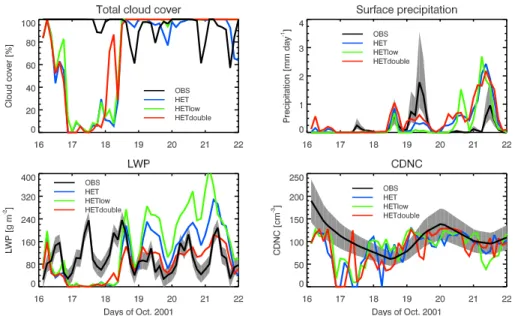
The stratocumulus cloud had a thickness between 200 m and 500 m and was present for the whole period (Fig. 3). The cloud fraction varied between 60% and 100%. Since the vertical resolution of the model is around 500 m, the vertical extension of the cloud 5

was equal or less the vertical resolution of the model. Hence, small amounts of pre-cipitation formed inside the cloud caused its decay. The period on 17 October with low cloud cover in all simulations could be due to problems in the representation of the me-teorological conditions by the forcing data (Posselt and Lohmann, 2008). From 18 Oc-tober onwards a higher cloud fraction is present in all model simulations. A reduction 10

of cloud cover is mainly calculated with simulation HET due to enhanced precipita-tion which strongly reduces LWP. In simulaprecipita-tions REF and HOM the model preferably calculates overcast conditions for the second part of the period.

The observed LWP shows a large variation with values between 0 and 250 g m−2 (Fig. 3). It shows a diurnal cycle and is also influenced by the precipitation formed 15

in the stratocumulus layer. Since the precipitation on 18 and 19 October is lower in the simulations REF and HOM (Fig. 3), LWP remains rather high. LWP in simulation HET is lower due to higher precipitation rates and the observed characteristics of LWP are better captured. In general, LWP in simulation HET shows better agreement with observations than simulations REF and HOM which can also be seen in the time aver-20

aged values for the whole period in Table 3. But the peaks are still overpredicted. During the period several precipitation events occur with a maximum of 1.8 mm day−1 on 19 October. The precipitation rates in the model simulations are underestimated during the first period, while in the second period beginning on 20 October all simula-tions strongly overpredict the measured rain rate at the surface (Fig. 3). Precipitation 25

(14)

ACPD

11, 9335–9374, 2011

S. Jess et al.

Title Page

Tables Figures

◭ ◮

Back Close

Full Screen / Esc

Discussion

P

a

per

|

Dis

cussion

P

a

per

|

Discussion

P

a

per

|

Discussio

n

P

a

per

|

the first time steps of the simulations precipitation strongly reduces the cloud fraction in all simulations (Fig. 3). While precipitation reaches the surface in simulation HET on 16 October, the evaporation rate is stronger in simulations REF and HOM and no precipitation was predicted at the surface. Differences in precipitation between simu-lations and observations can be caused by under- or overestimation of the internally 5

calculated surface fluxes (Posselt and Lohmann, 2008). On 20 October, precipitation forms earlier in simulation HET but also persists for a longer time because the inhomo-geneities are able to produce more continuous precipitation probably in di_fferent parts of the cloud. Hence the autoconversion and accretion rates are enhanced in simula-tion HET. A reducsimula-tion in the overestimasimula-tion of the peak precipitasimula-tion rates is simulated 10

in simulation HET on 20 October as compared to simulation REF and HOM because LWP is not as large in HET as in REF and HOM.

The observed CDNC is a layer-mean and shows high values at the beginning of the period probably caused by advection from the continent, followed by a decrease and a subsequent increase after the precipitation event on 19 October (Fig. 3). Simulated 15

CDNC is in the observed range in the second part of the period in all simulations and differences between the simulations are small.

Figures 4 and 5 show the relationship between LWP and precipitation as well as CDNC and precipitation from observations and the model simulations. The overesti-mation in LWP is reduced in simulation HET as compared to simulations REF and HOM 20

(Fig. 4). The spread in the simulations for the relationship precipitation and CDNC is larger than for precipitation and LWP (Fig. 5). The relationship between precipitation and LWP is closest to the observations for simulation HET. For the EPIC case the distinction between cloudy and cloud-free sub-boxes with the average cloud conden-sate according to Jakob and Klein (1999) (HOM) is not sufficient to affect the precip-25

(15)

ACPD

11, 9335–9374, 2011

S. Jess et al.

Title Page

Tables Figures

◭ ◮

Back Close

Full Screen / Esc

Discussion

P

a

per

|

Dis

cussion

P

a

per

|

Discussion

P

a

per

|

Discussio

n

P

a

per

|

LWP is reduced. Hence LWP in simulation HET is closer to the measurements than simulations REF and HOM.

4.2.2 MPACE period A – multi-layer cloud

The observations show a persistent multi-layer mixed-phase cloud during the whole time that extends up to approximately 500 hPa with a maximum thickness on 7 October 5

(Fig. 6). In all simulations a multi-layered cloud is present, but the modeled clouds are less continuous and have a smaller vertical extension than the observed cloud. The vertical thickness of the cloud is reduced in simulation HET as compared to simulations REF and HOM due to sedimentation of cloud ice.

The mixed-phase cloud produces precipitation rates with an observed maximum of 10

0.17 mm h−1on 7 October (Fig. 6). All simulations overestimate the precipitation rate on the first days of the simulation. They underpredict it on 7 October but the timing of the precipitation peak in simulation HET correlates quite well with the observations, while no precipitation peak is simulated for the simulations REF and HOM. The second precipitation event is captured quite well by all simulations. By including cloud inhomo-15

geneities an earlier precipitation formation and therefore a reduction of the cloud life time is triggered due to sedimentation of ice crystals in simulation HET. For the second precipitation event on 6 October more precipitation is formed in simulation HET which keeps LWP low (Fig. 6). The high overestimation of precipitation in all simulations at the beginning seems to be an initialization problem while the absence of precipitation 20

on 7 October may be caused by not considering the large-scale advection of hydrom-eteors in the forcing data (Morrison et al., 2009).

The observed LWP consists of two different retrieval methods. One is averaged be-tween the stations Barrow and Oliktok Point (WANG retrieval) and the other is averaged between the stations Barrow, Oliktok Point and Atquasuk (TURNER retrieval) (Turner 25

et al., 2007). Observations of LWP show lower values for the first days and a higher peak on 8 October with a maximum around 150 g m−2for the TURNER retrievals and 250 g m−2

(16)

ACPD

11, 9335–9374, 2011

S. Jess et al.

Title Page

Tables Figures

◭ ◮

Back Close

Full Screen / Esc

Discussion

P

a

per

|

Dis

cussion

P

a

per

|

Discussion

P

a

per

|

Discussio

n

P

a

per

|

overestimate LWP for the first days while simulation HET shows reduced values in better agreement with the observations. All simulations underpredict LWP on the last simulation day. While precipitation forms via the warm phase at the beginning of the simulations REF and HOM, some cold precipitation forms in case of simulation HET in accordance with observations reporting intermittent precipitation in form of light snow 5

(Morrison et al., 2009). However, the amounts of snow in simulation HET are quite low (not shown).

The observations of ice water path (IWP) are retrieved from RADAR measurements over the station Barrow (SHUPE-TURNER method) (Shupe et al., 2006) and show high values on 6 and 7 October with a maximum of approximately 250 g m−2 for 7 October 10

(Fig. 6). The model estimates of IWP do not include snow at the surface. The simula-tions REF and HOM are not able to form ice until 6 October. The first precipitation peak is partly diagnosed as snow in simulation HET, so the ice formed is already removed from the atmosphere. On 7 October less ice is formed in simulation HET due to more precipitation via the warm phase so that less cloud water is available for freezing. The 15

high amounts of ice in the atmosphere could not be captured in any simulation. Obser-vations report a higher LWP in the shallow cloud on 8 October and a lower LWP in the deeper cloud before. This suggests the impact of seeding of ice from above in reducing LWP in the deeper clouds (Morrison et al., 2009) which also seems to be a problem in the simulations. One probable reason could be that precipitation removes liquid water 20

too fast from the atmosphere so that less liquid water is available for the freezing pro-cess. Additionally, ice which formed within one time step may have sedimented and sublimate in subsaturated regions below the cloud. Also hydrometeor advection is not provided in the forcing data. Hydrometeor advection could have occurred on 7 October, where the observations show high amounts of LWP.

25

(17)

ACPD

11, 9335–9374, 2011

S. Jess et al.

Title Page

Tables Figures

◭ ◮

Back Close

Full Screen / Esc

Discussion

P

a

per

|

Dis

cussion

P

a

per

|

Discussion

P

a

per

|

Discussio

n

P

a

per

|

5 Sensitivity studies

5.1 Number of sub-columns

The distribution of cloud cover is sensitive to the number of chosen sub-columns. The more sub-columns the more accurate is the distribution of cloud cover. For example if the cloud cover is 0.73 and 20 sub-columns are used for the simulation, then 15 of 5

the 20 sub-columns are cloudy which corresponds to a cloud fraction of 0.75, while in the case of 30 sub-columns 22 out of 30 are cloudy which yields a cloud fraction of 0.733. In case more sub-boxes are cloudy, more precipitation can be formed which can influence the precipitation fraction and LWP. If less then 10 sub-columns are chosen, the cloud cover is distributed with an error that affects the distribution of mass and 10

number concentration inside the cloudy sub-boxes (not shown).

In a sensitivity test the number of sub-columns was changed from 20 sub-columns, which was used in the simulations described above, to values between 21 and 500 for the homogeneous distribution HOM. As compared to the reference run, a homoge-neous simulation with 20 sub-columns needs to 10% more CPU time for the di_fferent 15

cases. For 100 sub-columns the CPU time increases by 45% as compared to the reference version.

A change in the number of sub-columns for the simulation HET shows a stronger in-crease in the CPU time. As compared to the reference run, the time is inin-creased by 25 to 27% for the simulation with 20 sub-columns. For 40 sub-columns (60 sub-columns) 20

the time required is 46 to 52% (69 to 106%) higher than the CPU time consumed for REF. As explained in Sect. 3, a homogeneous distribution following Jakob and Klein (1999) is chosen if a distribution can not be found after some iterations. For the EPIC campaign about 10% of the water clouds are distributed homogeneously. 16% of the water clouds and 22% of the ice clouds are distributed homogeneously for the MPACE 25

(18)

ACPD

11, 9335–9374, 2011

S. Jess et al.

Title Page

Tables Figures

◭ ◮

Back Close

Full Screen / Esc

Discussion

P

a

per

|

Dis

cussion

P

a

per

|

Discussion

P

a

per

|

Discussio

n

P

a

per

|

Table 2 summarizes averaged values of cloud cover, LWP, CDNC and precipitation over the period with different number of sub-columns for the EPIC case. Changes in microphysical variables for HOM are small. The odd numbers of sub-columns were chosen to avoid the use of only multiples which produce the same cloud cover and therefore identical results. Largest changes occur between 20 and 21 sub-columns. 5

Here differences in cloud cover are the reason for changes occurring in the micro-physical variables. While the averaged values remain approximately the same, small changes occur in the distribution of LWP, CDNC and precipitation during time steps with a cloud cover smaller than overcast conditions. In general, the results converge for an increase in sub-columns, which is also true for simulation HET. Table 2 summarizes 10

examples for the heterogeneous distributions (HET20, HET40, HET60). Di_fferences between 20 and 60 sub-columns are small, while the changes in microphysical vari-ables between 20 and 40 sub-columns are larger due to an earlier increase in cloud cover to overcast conditions on 18 October.

For the MPACE campaign the high precipitation rate at the beginning dominates the 15

averaged cloud properties and therefore differences in the average values are small when changing the number of sub-columns. Due to mainly overcast conditions the sensitivity of the results to the number of sub-columns is even smaller as compared to the EPIC case.

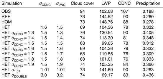
5.2 Standard deviation of the distributions

20

In order to evaluate the impact of the chosen standard deviations for the distributions of mass and number concentrations on the precipitation formation, the applied stan-dard deviations σ_LWC₌_{1.5 for and} σ_CDNC₌_1.6, σ_IWC₌_{1.25 and} σ_ICNC₌_{1.1 are all}

set toσ_CDNC₌σ_LWC₌σ_IWC₌σ_ICNC₌1.01 in the simulation HET20 low and doubled in simulation HET20 double to σ_LWC₌_3.0, σ_CDNC₌_3.2, σ_IWC₌_{2.5 and} σ_ICNC₌_{2.2. To}

25

(19)

ACPD

11, 9335–9374, 2011

S. Jess et al.

Title Page

Tables Figures

◭ ◮

Back Close

Full Screen / Esc

Discussion

P

a

per

|

Dis

cussion

P

a

per

|

Discussion

P

a

per

|

Discussio

n

P

a

per

|

For the MPACE case another experiment was performed where the standard devia-tions for LWC, IWC and CDNC were fixed but the standard deviation for ICNC is varied from a constant value of 1.1 to values between 1.2 and 1.7.

For a small value ofσ the distribution is narrow and is closer to the simulation HOM while for a higherσ _{the distribution becomes broader and a larger range of values is}

5

allowed in the different sub-columns.

5.2.1 EPIC

The cloud cover for the narrow distribution (HETlow) follows simulation HET for the first part of the simulation but shows mainly overcast conditions for the second period of the simulation (Fig. 7). For the broader distribution of cloud properties (HETdouble) 10

the cloud thickens earlier as compared to the other simulations and mainly overcast conditions dominate during the second part of the simulation as well. The averaged precipitation over the period is higher in simulation HETdouble but simulation HETlow is comparable to simulation HOM where less precipitation is formed at the beginning but more on the last simulation days (see also Table 3). LWP is enhanced in simulation 15

HETlow because the subgrid variability is reduced and the results are close to simula-tion HOM with less precipitasimula-tion at the beginning. Due to a higher precipitasimula-tion rate in simulation HETdouble LWP is consequently lower.

Ifσ_CDNC_{is changed only (Fig. 8), the timing of cloud thickening on 18 October is}

af-fected due to changes in the onset and amount of precipitation. In general, the changes 20

in LWP are smaller for this sensitivity study as compared to changes between the sim-ulations REF and HOM (Table 3). Largest differences occur for the smallest standard deviation. Since the autoconversion rate is proportional to LWC2.5 and CDNC−1.8 in the used parameterization, changes in LWP dominate for a small spread in σ_CDNC. Differences in CDNC are small and show no clear trend.

25

(20)

ACPD

11, 9335–9374, 2011

S. Jess et al.

Title Page

Tables Figures

◭ ◮

Back Close

Full Screen / Esc

Discussion

P

a

per

|

Dis

cussion

P

a

per

|

Discussion

P

a

per

|

Discussio

n

P

a

per

|

the higher the probability that precipitation is formed in at least one cloudy sub-box resulting in an earlier onset of precipitation at the surface. This can be observed on 20 October, where the precipitation onset is shifted to a later time when the standard deviation is reduced (Fig. 7). A change inσ_CDNC_{mainly a}_ff_{ects the cloud cover and the}

onset and amount of precipitation. 5

5.2.2 MPACE period A – multi-layer cloud

Since the amount of ice is low during MPACE A the sensitivity in IWP is negligible when onlyσ_ICNC _{is changed, while di}_ff_{erences in precipitation are directly linked to changes}

in LWP. The first precipitation peak is not a_ffected by a change inσ_ICNC.

A larger spread between the different sensitivity simulations can be observed for 10

a simple change inσ_CDNC_a_ff_{ecting IWP, LWP and precipitation. Again the smallest and}

the largest standard deviations show the greatest impact with increased precipitation for the first peak. For σ_CDNC₌₁._{3 more precipitation is caused via sedimentation of}

cloud ice and increased warm rain formation while for simulation σ_CDNC₌₁._{9 more}

precipitation via the warm phase leads to enhanced surface precipitation. If a broader 15

distribution is used for both mass and number concentration more precipitation forms at an earlier time which reduces LWP. The sedimentation of cloud ice is reduced which increases the cloud life time. One reason is that in boxes containing a large number concentration of ice crystals the terminal velocity is low. Hence ice crystals stay in the layer. On the opposite a narrow distribution leads to less ice formation at the beginning 20

and therefore a higher LWP but later on the freezing rate is enhanced.

In summary, a change inσ_ICNC _{leads to small changes in cloud microphysical}

prop-erties since IWP is low while a change in σ_CDNC _a_ff_{ects the freezing and}

precipi-tation rate because autoconversion and freezing depends on the size of the cloud droplets. A change in the standard deviations of mass and number concentration at 25

(21)

ACPD

11, 9335–9374, 2011

S. Jess et al.

Title Page

Tables Figures

◭ ◮

Back Close

Full Screen / Esc

Discussion

P

a

per

|

Dis

cussion

P

a

per

|

Discussion

P

a

per

|

Discussio

n

P

a

per

|

5.3 Variation in vertical correlation

In order to evaluate the choice of the vertical correlation, two different sensitivity simula-tions were performed where first no correlation between the cloud properties in different layers (HETcor₌0) and second a perfect correlation (HETcor₌1) is assumed. For the perfect correlation the same mass and/or number concentration of water and ice is 5

filled into the sub-box directly below if both layers are cloudy. The properties of the last cloudy sub-box of each level are chosen that the average values are conserved.

Figure 9 shows the changes in cloud properties for different assumptions of the ver-tical correlation for the EPIC campaign. It can be seen that changes occur but they are smaller than the differences between the simulations REF and HOM and the diff er-10

ences when changing the standard deviation.

Larger changes occur in case of the multi-layer mixed-phase cloud from the MPACE campaign (Fig. 10). While changes in LWP are rather small, a strong increase in precipitation is seen in the simulation without vertical correlation, which is caused by enhanced accretion on 6 October and first enhanced freezing and second stronger 15

sedimentation of cloud ice through the cloud on 7 October. The reason for the large difference between the simulations is a low ice water mixing ratio in the upper cloudy levels. If the correlation between the levels is assumed to be high, then the same IWC is filled into the lower level and the majority of sub-boxes contain only small amounts of IWC while only few boxes have larger amounts of cloud ice where the ice crystals 20

may sublimate below the cloud. The simulations HET and HETcor=1 are similar since there is a strong correlation between the vertical levels probably caused by low wind shear.

In summary, the vertical correlation seems to be less important for a water cloud only, because cloud droplets do not sediment in the ECHAM model due to low terminal 25

(22)

ACPD

11, 9335–9374, 2011

S. Jess et al.

Title Page

Tables Figures

◭ ◮

Back Close

Full Screen / Esc

Discussion

P

a

per

|

Dis

cussion

P

a

per

|

Discussion

P

a

per

|

Discussio

n

P

a

per

|

6 Conclusions

In this paper a statistical sub-column algorithm was included into the ECHAM5 SCM for a more physical treatment of subgrid variability in precipitation formation. Each column of the model is divided into 20 sub-columns, which are independent and contain random microphysical values from log-normal distributions (simulation HET).

5

The precipitation formation and changes in microphysical variables were investigated for a liquid cloud in the tropics (EPIC campaign) and a multi-layer mixed-phase cloud over Alaska (MPACE campaign) to evaluate the algorithm.

The simulations show an increase in the precipitation efficiency due to the inhomo-geneities at the beginning of the simulation. For the EPIC field campaign the new 10

algorithm was able to produce a higher precipitation rate earlier and a reduced LWP in better agreement with the observations. In simulation HET for MPACE A the vertical extension of the cloud was reduced due to sedimentation of ice. In the first time steps precipitation falls as snow as observed during the campaign. The inhomogeneities led to an enhanced precipitation rate over several time steps. In general, simulation HET 15

shows no improvement as compared to the reference simulation for the MPACE case. Sensitivity studies showed a small sensitivity to a change in the number of sub-columns for the homogeneous distribution for both campaigns. A change in the distri-bution width shows a large sensitivity. The narrow distridistri-bution is close to the simulation HOM following Jakob and Klein (1999). The vertical correlation between cloud layers is 20

less important for the EPIC campaign, but the presence of ice crystals and enhanced accretion inside the mixed-phase cloud of the MPACE campaign yields a larger sen-sitivity to the vertical correlation but mainly in terms of the precipitation amount and IWP. Especially for the EPIC campaign, the inhomogeneities in simulation HET are necessary to form more precipitation.

25

(23)

ACPD

11, 9335–9374, 2011

S. Jess et al.

Title Page

Tables Figures

◭ ◮

Back Close

Full Screen / Esc

Discussion

P

a

per

|

Dis

cussion

P

a

per

|

Discussion

P

a

per

|

Discussio

n

P

a

per

|

that the chosen standard deviations are valid for all clouds in the GCM. With the more physical treatment of precipitation in the sub-columns the washout of aerosols needs to be treated accordingly. This will have implications for the indirect aerosol effect. Improvements may account for a more consistent treatment of the statistical cloud cover scheme and distribution of cloud properties. Further the algorithm could be 5

coupled with the radiation parameterization for which the cloud fraction is an important parameter. Also subgrid variability strongly influences the optical thickness of a cloud (Carlin et al., 2002; Pincus et al., 2006). Our method coupled to the radiation routine as introduced by R ¨ais ¨anen et al. (2004) should save computing time as compared to the use of a high-resolution model (Grabowski, 2001) because only the cloudy columns 10

will be divided into sub-columns. Furthermore it might be possible to improve the precipitation formation and reduce errors in the radiation budget and distribution of precipitation.

Acknowledgements. We want to thank Martina Kr ¨amer from Forschungszentrum J ¨ulich (Ger-many), Hugh Morrison from National Center for Atmospheric Research, Boulder, Colorado

15

(USA), Matthew D. Shupe from Cooperative Institute for Research in Environmental Sciences, University of Colorado/NOAA, Boulder, Colorado (USA), Zhien Wang from Department of At-mospheric Science, University of Wyoming (USA) and David D. Turner from Space Science and Engineering Center, University of Wisconsin (USA) for providing us data and also Sylvaine Ferrachat for technical support.

20

References

Baker, M. B.: Cloud microphysics and climate, Science, 276(5315), 1072–1078, 1997. 9338 Barker, H. W., Pincus, R., and Morcrette, J. J.: The Monte Carlo independent column

approxi-mation: application within largescale models, paper presented at the GCSS-ARM Workshop on the Representation of cloud systems in large-scale models, global energy and water

cy-25

(24)

ACPD

11, 9335–9374, 2011

S. Jess et al.

Title Page

Tables Figures

◭ ◮

Back Close

Full Screen / Esc

Discussion

P

a

per

|

Dis

cussion

P

a

per

|

Discussion

P

a

per

|

Discussio

n

P

a

per

|

Bretherton, C., Uttal, T., Fairall, C., Yuter, S., Weller, R., Baumgardner, D., Comstock, K., Wood, R., and Raga, G.: The EPIC 2001 stratocumulus study, B. Am. Meteorol. Soc., 85, 967–977, 2004. 9340, 9345

Carlin, B., Fu, Q., Lohmann, U., Mace, G. G., Sassen, K., and Comstock, J. M.: High-cloud horizontal inhomogeneity and solar albedo bias, J. Climate, 15, 2321–2339, 2002. 9337,

5

9357

Chahine, M. T.: The hydrological cycle and its influence on climate, Nature, 359, 373–380, 1992. 9337

Comstock, J. M., Wood, R., Yuter, S. E., and Bretherton, C. S.: Reflectivity and rain rate in and below drizzling stratocumulus, Q. J. Roy. Meteor. Soc., 130, 2891–2919, 2004. 9345

10

Dong, X. and Mace, G. G.: Profiles of low-level stratus cloud microphysics deduced from ground-based measurements, J. Atmos. Ocean. Tech., 20, 42–53, 2003. 9345

Gayet, J.-F., Ovarlez, J., Shcherbakov, V., Str ¨om, J., Schuhmann, U., Minikin, A., Auriol, F., Petzold, A., and Monier, M.: Cirrus cloud microphysical and optical properties at southern and northern midlatitudes during the INCA experiment, J. Geophys. Res., 109, D20206,

15

doi:10.1029/2004JD004803, 2004. 9344

Grabowski, W. W.: Coupling cloud processes with the large-scale dynamics using the cloud-resolving convection parameterization (CRCP), J. Atmos. Sci., 58, 978–997, 2001. 9339, 9340, 9357

Gultepe, I. and Isaac, G. A.: Liquid water content and temperature relationship from aircraft

20

observations and its applicability to GCMs, J. Climate, 10, 446–452, 1996. 9344

Gultepe, I. and Isaac, G. A.: Aircraft observations of cloud droplet number concentration: im-plications for climate studies, Q. J. Roy. Meteor. Soc., 130, 2377–2390, 2004. 9344

Hogan, R. J. and Illingworth, A. J.: Parameterizing ice cloud inhomogeneity and the overlap of inhomogeneities using cloudradar data, J. Atmos. Sci., 60, 756–767, 2003. 9342

25

Hogg, D. C., Guiraud, F. O., Snider, J. B., Decker, M. T., and Westwater, E. R.: A steerable dual-channel microwave radiometer for the measurements of water vapor and liquid in the troposphere, J. Appl. Meteorol., 22, 789–806, 1983. 9345

Jakob, C. and Klein, S. A.: The role of vertically varying cloud fraction in the parameterization of microphysical processes in the ECMWF model, Q. J. Roy. Meteor. Soc., 125, 941–965,

30

1999. 9339, 9340, 9341, 9342, 9343, 9344, 9348, 9351, 9356, 9362

(25)

ACPD

11, 9335–9374, 2011

S. Jess et al.

Title Page

Tables Figures

◭ ◮

Back Close

Full Screen / Esc

Discussion

P

a

per

|

Dis

cussion

P

a

per

|

Discussion

P

a

per

|

Discussio

n

P

a

per

|

Khairoutdinov, M. and Kogan, Y.: A new cloud physics parameterization in a large-eddy simu-lation model of marine stratocumulus, Mon. Weather Rev., 128, 229–243, 2000. 9341 Kiehl, J. T. and Trenberth, K. E.: Earth’s annual global mean energy budget, B. Am. Meteorol.

Soc., 78, 197–208, 1997. 9337

Klein, S. A., McCoy, R. B., Morrison, H. , Ackerman, A. S., Avramov, A., de Boer, G., Chen, M.,

5

Cole, J. N. S., Del Genio, A. D., Falk, M., Foster, M. J., Fridlind, A., Golaz, J.-C., Hashino, T., Harrington, J. Y., Hoose, C., Khairoutdinov, M. F., Larson, V. E., Liu, X., Luo, Y., McFar-quhar, G. M., Menon, S., Neggers, R. A. J., Park, S., Poellot, M. R., Schmidt, J. M., Sednev, I., Shipway, B. J., Shupe, M. D., Spangenberg, D. A., Sud, Y. C., Turner, D. D., Veron, D. E., von Salzen, K., Walker, G. K., Wang, Z., Wolf, A. B., Xie, S., Xu, K.-M., Yang, F., and

10

Zhang, G.: Intercomparison of model simulations of mixed-phase clouds observed during the ARM Mixed-phase Arctic Cloud Experiment, Part I: Single layer cloud, Q. J. Roy. Meteor. Soc., 135, 979–1002, 2009. 9346

Larson, V. E., Wood, R., Field, P. R., Golaz, J.-C., Haar, T. H. V., and Cotton, W. R.: Systematic biases in the microphysics and thermodynamics of numerical models that ignore

subgrid-15

scale variability, J. Atmos. Sci., 58, 1117–1128, 2001. 9337

Lohmann, U. and Roeckner, E.: Design and performance of a new cloud microphysics scheme developed for the ECHAM general circulation model, Clim. Dynam., 12, 557–572, 1996. 9341

Lohmann, U., Spichtinger, P., Jess, S., Peter, T., and Smit, H.: Cirrus clouds and ice

super-20

saturated regions in a global climate model, Environ. Res. Lett., 3 (4), doi:10.1088/1748-9326/3/4/045022, 2008. 9341, 9344

Manton, M. J. and Cotton, W. R.: Formulation of approximate equations for modeling moist deep convection on the mesoscale, Atmos. Sci. Pap., 266, Dep. Atmos. Sci., Colo. State Univ., Fort Collins, 1977. 9337

25

Morrison, H. and Gettelman, A.: A new two-moment bulk stratiform cloud microphysics scheme in the community atmosphere model, Version 3 (CAM3), Part I: Description and numerical tests, J. Climate, 21, 3642–3659, 2008. 9337

Morrison, H., McCoy, R. B., Klein, S. A., Xie, S., Luo, Y., Avramov, A., Chen, M., Cole, J. N. S., Falk, M., Foster, M. J., Del Genio, A. D., Harrington, J. Y., Hoose, C., Khairoutdinov, M. F.,

30

(26)

ACPD

11, 9335–9374, 2011

S. Jess et al.

Title Page

Tables Figures

◭ ◮

Back Close

Full Screen / Esc

Discussion

P

a

per

|

Dis

cussion

P

a

per

|

Discussion

P

a

per

|

Discussio

n

P

a

per

|

clouds observed during the ARM Mixed-Phase Arctic Cloud Experiment, Part II: Multilayer cloud, Q. J. Roy. Meteor. Soc., 135, 1003–1019, 2009. 9346, 9349, 9350

Pincus, R., McFarlane, S. A., and Klein, S. A.: Albedo bias and the horizontal variability of clouds in subtropical marine boundary layers: observations from ships and satellites, J. Geo-phys. Res., 104(D6), 6183–6191, 1999. 9337

5

Pincus, R., Barker, H. W., and Morcrette, J. J.: A fast, flexible, approximate technique for computing radiative transfer in inhomogeneous cloud fields, J. Geophys. Res., 108, 4376, doi:10.1029/2002JD003322, 2003. 9339

Pincus, R., Hemler, R., and Klein, S. A.: Using stochastically generated subcolumns to rep-resent cloud structure in a large-scale model, Mon. Weather Rev., 134, 3644–3656, 2006.

10

9357

Posselt, R. and Lohmann, U.: Introduction of prognostic rain in ECHAM5: design and single column model simulations, Atmos. Chem. Phys., 8, 2949–2963, doi:10.5194/acp-8-2949-2008, 2008. 9347, 9348

R ¨ais ¨anen, P., Barker, H. W., Khairoutdinov, M. F., Li, J., and Randall, D. A.: Stochastic

gener-15

ation of subgrid-scale cloudy columns for large-scale models, Q. J. Roy. Meteor. Soc., 130, 2047–2068, 2004. 9339, 9340, 9343, 9357

Raschke, E., Ohmura, A., Rossow, W. B., Carlson, B. E., Zhang, Y.-C., Stubenrauch, C., Kot-tek, M., and Wild, M.: Cloud effects on the radiation budget based on ISCCP data (1991 to 1995), Int. J. Climatol., 25, 1103–1125, 2005. 9337

20

Roeckner, E., B ¨auml, G., Bonaventura, L., Brokopf, R., Esch, M., Giorgetta, M., Hagemann, S., Kirchner, I., Kornblueh, L., Manzini, E., Rhodin, A., Schlese, U., Schulzweida, U., and Tomp-kins A. : The atmospheric general circulation model ECHAM5, Part I: Model description, Report 349, Max Planck Institute for Meteorology, Hamburg, Germany, 2003. 9341

Rotstayn, L. D.: On the “tuning” of autoconversion parameterizations in climate models, J.

Geo-25

phys. Res., 105, doi:10.1029/2000JD900129, 15495–15507, 2000. 9337

Schiller, C., Kr ¨amer, M., Afchine, A., Spelten, N., and Sitnikov, N.: The ice water con-tent of Arctic, mid latitude and tropical cirrus, J. Geophys. Res., 113(D24208), 12 pp., doi:10.1029/2008JD010342, 2008. 9344

Shupe, M. D., Matrosov, S. Y., and Uttal, T.: Arctic mixed-phase cloud properties derived from

30

surface-based sensors at SHEBA, J. Atmos. Sci., 63, 697–711, 2006. 9350

(27)

aerosol-ACPD

11, 9335–9374, 2011

S. Jess et al.

Title Page

Tables Figures

◭ ◮

Back Close

Full Screen / Esc

Discussion

P

a

per

|

Dis

cussion

P

a

per

|

Discussion

P

a

per

|

Discussio

n

P

a

per

|

climate model ECHAM5-HAM, Atmos. Chem. Phys., 5, 1125–1156, doi:10.5194/acp-5-1125-2005, 2005. 9341

Tompkins, A.: A prognostic parameterization for the subgrid-scale variability of water vapor and clouds in large scale models and its use to diagnose cloud cover, J. Atmos. Sci., 59(12), 1917–1942, 2002. 9339, 9341

5

Tsushima, Y., Emori, S., Ogura, T., Kimoto, M., Webb, M. J., Williams, K. D., Ringer, M. A., Soden, B. J., Li, B. und Andronova, N.: Importance of the mixed-phase cloud distribution in the control climate for assessing the response of clouds to carbon dioxide increase: a multi-model study, Clim. Dynam., 27, 113–126, 2006. 9338

Turner, D., Clough, S., Liljegren, J., Clothiaux, E., Cady-Pereira, K., and Gaustad, K.: Retrieving

10

liquid water path and precipitable water vapor from the atmospheric radiation measurement (ARM) microwave radiometers, IEEE T. Geosci. Remote, 45, 3680–3690, 2007. 9349 Verlinde, J., Harrington, J. Y., McFarquhar, G. M., Yannuzzi, V. T., Avramov, A., Greenberg, S.,

Johnson, N., Zhang, G., Poellot, M. R., Mather, J. H., Turner, D. D., Eloranta, E. W., Zak, B. D., Prenni, A. J., Daniel, J. S., Kok, G. L., Tobin, D. C., Holz, R., Sassen, K.,

15

Spangenberg, D., Minnis, P., Tooman, T. P., Ivey, M. D., Richardson, S. J., Bahrmann, C. P., Shupe, M.,DeMott, P. J., Heymsfield, A. J. and Schofield, R. : The mixed-phase arctic cloud experiment, B. Am. Meteorol. Soc., 88, 205–221, 2007. 9340, 9346

Weinman, J. A. and Swarztauber, P. N.: Albedo of a stratified medium of isotropically scattering particles, J. Atmos. Sci., 25, 497–501, 1968. 9338

20

(28)

ACPD

11, 9335–9374, 2011

S. Jess et al.

Title Page

Tables Figures

◭ ◮

Back Close

Full Screen / Esc

Discussion

P

a

per

|

Dis

cussion

P

a

per

|

Discussion

P

a

per

|

Discussio

n

P

a

per

|

Table 1.Set-up for the three different single column model simulations.

Simulation Description

REF Reference simulation with the original model ECHAM5.5 with a changed order of the cloud microphysical processes (see Sect. 2)

HOM As simulation REF but 20 sub-columns with a homogeneous distribution following Jakob and Klein (1999) (the mean

cloud condensate is used for each cloudy sub-box of each layer)

(29)

ACPD

11, 9335–9374, 2011

S. Jess et al.

Title Page

Tables Figures

◭ ◮

Back Close

Full Screen / Esc

Discussion

P

a

per

|

Dis

cussion

P

a

per

|

Discussion

P

a

per

|

Discussio

n

P

a

per

|

Table 2. Sensitivity studies for the EPIC campaign with the single column model for different number of sub-columns: for HET20 the following standard deviations are used: σ_LWC₌1.5,

σ_CDNC₌1.6. The values are given as cloud cover (%), liquid water path (LWP) (g m−2

), cloud droplet number concentration (CDNC) (cm−3) and precipitation (mm day−1).