How large is the spreading width of a superdeformed band?
A. N. Wilson,1,2,∗A. J. Sargeant,3P. M. Davidson,1and M. S. Hussein3
1Department of Nuclear Physics, Research School of Physical Sciences and Engineering, Australian National University, Canberra, ACT 0200, Australia
2Department of Physics and Theoretical Physics, Faculty of Science, Australian National University, Canberra, ACT 0200, Australia 3Instituto de F´ısica, Universidade de S˜ao Paulo, Caixa Postal 66318, 05315-970 S˜ao Paulo, SP, Brazil
(Received 21 May 2004; published 30 March 2005)
Recent models of the decay out of superdeformed (SD) bands can broadly be divided into two categories. One approach is based on the similarity between the tunneling process involved in the decay and that involved in the fusion of heavy ions, and it builds on the formalism of nuclear reaction theory. The other arises from an analogy between the superdeformed decay and transport between coupled quantum dots. These models suggest conflicting values for the spreading width of the decaying superdeformed states. In this paper, the decay of superdeformed bands in the five even-even nuclei in which the SD excitation energies have been determined experimentally is considered in the framework of both approaches, and the significance of the difference in the resulting spreading widths is considered. The results of the two models are also compared to tunneling widths estimated from previous barrier height predictions and a parabolic approximation to the barrier shape.
DOI: 10.1103/PhysRevC.71.034319 PACS number(s): 23.20.Lv, 27.80.+w, 21.10.Re
I. INTRODUCTION
Superdeformed (SD) nuclei are associated with a second minimum in the nuclear potential occurring at large deforma-tion. The excited superdeformed well is separated from the primary minimum (associated with “normal” nuclear shapes) by a real potential barrier. Rotational SD bands have now been observed in several groups of nuclei with masses ranging fromA≈20 toA≈240 [1]. Although each region displays distinct characteristics which depend on the underlying nuclear structure supporting the large deformations, there are some features which are common to all SD bands. Perhaps the most interesting of these is the abrupt decay out of the SD bands to levels of normal deformation: complete loss of intensity usually occurs over only two or three consecutive levels.
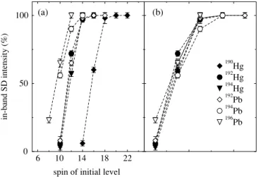
In this paper, we focus on the decay of SD bands with masses A≈190 and A≈150, which are considered to be two of the classic “islands of superdeformation.” In these two regions, the extreme deformation is not driven by a small number of specific single-particle orbitals but is instead the result of the complex interplay of macroscopic (Coulomb and rotational) and microscopic (shell structure) effects. Theoretical calculations indicate that two distinct minima associated with SD and normal nuclear shapes are present at the point of decay in these nuclei, unlike, for example, the triaxial superdeformed bands observed in theA≈160 region. Indeed, in theA≈190 region, the SD minimum is thought to exist even at zero rotational frequency. Thus, it is in these cases that it is clearest that the decay occurs via a barrier penetration process. The intensity profiles of six superdeformed bands in isotopes of Hg and Pb are shown in Fig. 1; the data have been taken from Refs [2–7]. The decay patterns are all remarkably similar, despite the different excitation energies and spins of the levels from which the decay occurs.
∗E-mail address: [email protected]
The possible causes of this rapid loss of flux have been the subject of much discussion, but despite more than a decade of theoretical and experimental work, no complete theory of the decay mechanism has been achieved. Indeed, it is as yet not clear whether the sudden enhancement of the decay probability is due to the dependence on angular momentum of the height of the barrier separating the SD and normal potential wells, to the increasing effect of pairing correlations with decreasing spin, or to the onset of chaos in the structure of the normal-deformed (ND) states [8]. One of the obstacles to progress in the attempt to understand the decay mechanism has been the difficulty of arriving at a consistent, broadly applicable, and reliable means of characterizing the size of the interaction between the SD and ND states involved in the decay out.
Recently, two conflicting approaches to the problem have been proposed which are derived from different assumptions concerning the mixing of SD and ND states (statistical and two-level mixing). The conflict manifests itself in the spreading widthsevaluated for the decaying SD levels, which differ by several orders of magnitude depending on which model is applied. It has been suggested [9] that these differences are not important, as the interaction strengths obtained in analyses of real data are similar [9,10]. However, there are several reasons to give the issue serious consideration.
First, the spreading width associated with a particular process is related to the strength of the interaction involved. In the case of the decay out of the superdeformed well, the relevant interactions are the strong force (in the rearrangement of the nucleons) and the electromagnetic force (in the emission of theγray from the decaying SD level to the lower-lying ND level). The spreading widths arrived at via the two models of the decay differ by orders of magnitude. Equally important, the parameters on which the spreading widths depend strongly are different within the two approaches, further indicating their incompatibility.
6 10 14 18 spin of initial level 0
50 100
in-band SD intensity (%)
190 Hg 192
Hg 194
Hg 192
Pb 194
Pb 196
Pb
(a) (b)
22
FIG. 1. Decay profiles of the yrast superdeformed bands in190Hg, 192Hg,194Hg,192Pb,194Pb, and196Pb. The right-hand panel shows the
profiles shifted in spin so that the last point represents the lowest spin level from below which some intensity remains in the band, regardless of the absolute spin.
of the potential barrier separating the superdeformed and normal minima, which should be comparable with theoretical predictions.
Third, we want to determine which of the two models, which have different physical bases and purport to describe the same phenomenon, is a more appropriate description of the SD decay. The concept of a spreading width has proved extremely useful in understanding other issues, such as parity violation, giant multipole resonances, isobaric analog states, and compound nucleus reactions, and so may help to distinguish between the two types of model discussed here.
It is the aim of the following to apply these models to decaying SD levels in nuclei withA≈190 andA≈150 and to consider the implications of the results. We apply two versions of a statistical mixing model and one of a simpler two-level mixing model to all of the yrast SD bands in even-even nuclei for which excitations and spins have been established. This is the first time that all the available data have been treated simultaneously, and it is also the first time that one of the two statistical models has been applied to real data.
II. DESCRIPTIONS OF THE DECAY FROM THE SUPERDEFORMED WELL
Before examining the decay profiles of the bands, it is useful to summarize the features shared by each of the models and to look at the differences in the structures of the two classes of model.
A. General assumptions
There are several basic assumptions common to all treat-ments of the SD decay-out process:
(i) The potential barrier separating the SD and ND minima is still present at the point of decay;
(ii) The decaying SD states are highly excited relative to the yrast (lowest energy for a given spin) ND states;
matrix element
ND states of the
same spinI
mixes SD and
extremely low level density in the SD well
ND state decays to many other ND states
ND Γ
SD
I - 1 I
I, I,
V V
high level density in the ND well
Γ
FIG. 2. Schematic illustration of the SD and ND levels at the point of decay.
(iii) The density of ND states at the same excitation energy and spin as the decaying SD states is high;
(iv) The decaying SD state couples to one or more of these excited ND states, thus allowing decay to lower-lying states in the primary minimum.
The decay is illustrated schematically in Fig. 2.
In general,I, the fractional intensity remaining in the SD band below a certain level, is described as depending on four parameters:ŴS, the width forγdecay within the SD band;ŴN,
the width forγ decay of states in the ND well;D, the average level spacing in the ND well andŴ↓, the spreading width of
the decaying SD state. This last quantity measures the fraction of the SD wavefunction extending to the ND well and should reflect the size of the barrier separating the two minima.
B. Statistical model
Recently, a framework originally developed for the study of compound nuclear reactions has been used to derive the in-and out-of-bin-and SD intensities. This approach has developed along two strands: (i) the ensemble-averaging technique of Gu and Weidenm¨uller [11] (GW), and (ii) the energy-averaging technique of Sargeant, Hussein, and collaborators [12] (SH). By the ergodic theorem, one expects the two averaging techniques to be equivalent. However, although the models are conceptually equivalent, differences in the derivations— for example, the SH derivation is strictly valid only in the overlapping resonance regime—mean that their results will differ in physically realistic cases. For this reason, it is interesting to see how rapidly the SH approach deviates from the more widely applicable GW approach. For details of the differences between the formulations, see Refs. [11,12].
In these statistical mixing models, the ND states are assumed to be compound, highly mixed states which can essentially be treated as “structure-free.” The mixing between an SD state and many equivalent energy ND states is described statistically; an SD state is assumed to couple with equal strength to all ND states with the same spin, since their compound nature implies that there will be no states with wavefunctions which have a significant overlap with the wavefunction of the pure SD states. The ND states are described by the Gaussian orthogonal ensemble (GOE), and the decomposition
ave
D ∆
(a) (b)
i j k l m
0 V
V V V
V
V
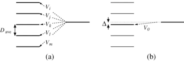
FIG. 3. (a) In the statistical models, the SD level mixes with many ND levels of average separationD. The resulting interactionVis an average over all of these interactions. (b) In the two-level mixing model, the SD level mixes predominantly with one ND level. The resulting interactionVis extracted assuming an average separation of the SD and ND states by energy=D/4.
is made, where Iav is an average component and Ifl is a fluctuating part. This is in direct analogy with compound nucleus reactions, where the cross section is described by average and fluctuating (Hauser-Feshbach) components. The mixing described by these statistical models is illustrated schematically in Fig. 3(a).
Both GW and SH yield
Iav=(1+Ŵ↓/ ŴS)−1, (2)
which depends only on the properties of the decaying SD state. As is the case in other fields where a statistical approach is appropriate (such as reaction theory and atomic physics), the spreading width is defined by
Ŵ↓=2πV2/D, (3)
whereVis the mean interaction matrix element of the SD state under study and the many nearby ND states.
The fluctuating partIfldepends additionally on the prop-erties of the ND states (the average level separationD and theγ-decay widthŴN). The GW approach, which uses
super-symmetry techniques to make a precise ensemble averaging, results in a nonanalytic expression for the fluctuating part of the intensity. A fit to the results of numerical evaluations led to the expression
IflGW =[1−0.9139(ŴN/D)0.2172]
×exp
−[0.4343 lnŴ↓/ Ŵ
S−0.45(ŴN/D)−0.1303]2
(ŴN/D)−0.1477
.
(4) The exact (nonanalytic) result of GW is valid for all values of ŴN/D (that is, not only for systems where the ND
states approach the overlapping resonance region but also for systems where the ND states are well separated and narrow). Equation (4) may not be valid for all ND conditions but is expected to be accurate within 20% for ŴN/D≈10−4 [9],
which is close to the conditions in some real SD decays. The SH approach yields the analytic expression
IflSH =2D/(π ŴN)Iav(1−Iav)2, (5) withIavgiven by Eq. (2). This expression is strictly valid only in the limit of strongly overlapping compound resonances but agrees well the GW expression down toŴN/D∼0.1. Below
this, the SH model may not provide a good approximation to the decay.
For all experimentally determined cases, the fluctuating part of the intensity is found to be the dominant contribution.
SH also derived the expression (I)2=I
fl 2
f1(ξ)+2IavIflf2(ξ) (6) for the mean variance ofI, which is an energy-integrated ver-sion of the Ericson fluctuation two-point intensity correlation function. In principle, Eq. (6) permits an assessment of the accuracy with which Ŵ↓ andVcan be extracted for specific values ofŴS,ŴN, I, andD. The functionsf1andf2are simple rational functions ofξ=ŴN/(ŴS+Ŵ↓).
C. Two-level mixing model
An alternative approach, initially presented by Stafford and Barrett [13] (SB), arose from an analogy between the SD decay and transport between coupled quantum dots. This is essentially a two-state mixing model, in which the coupling between the SD and ND states is described in a Green’s function formalism. The in-band intensity is described by a single component; in this case, the model describes the situation illustrated in Fig. 3(b). The expression for the in-band intensityIgiven by Cardamone, Stafford, and Barrett [14] can be rearranged to obtain
I =
1+Ŵ↓SB ŴS
ŴN
Ŵ↓SB+ŴN −1
. (7)
The authors of the SB approach state that the correct expression for the spreading width from applying Fermi’s Golden Rule in this model gives a tunneling rate
Ŵ↓SB=V2 ŴS+ŴN 2+(Ŵ
S+ŴN)2/4
, (8)
whereis the energy difference between the interacting ND and SD states. Here,Vis the interaction energy of an SD state with a single ND state (as opposed to a mean value defined by averaging over the interaction of an SD state with many ND states). WhenVis extracted from the data, the unknown quantityis replaced by an average SD-ND level separation given by|| =D/4. Thus, not only are the spreading widths derived in the two models quite different quantities, as is clear from their different definitions, but so too are the interaction energiesVandV.
D. Which class of model is a more appropriate description of real superdeformed bands?
Although the above models have been developed to repre-sent the same phenomenon, it can be seen that the statistical and two-level mixing models describe different physical situations and therefore should not necessarily be expected to produce reconcilable results. In fact, their application to real data yields very different values for the spreading widthsŴ↓andŴ↓
energies significantly lower than the overlapping resonance region for the ND levels. One might thus expect the SD state to mix predominantly with only a few ND levels. In such circumstances, does a two-state mixing model provide a better description than a fully statistical model?
An understanding of which type of model is correct is necessary before a deeper analysis of the implica-tions of existing data can be made. Given the present dearth of experimental data establishing excitation energies and spins of SD levels, one of the few experimental features which might be used to interrogate the models is the similarity of the SD bands’ intensity profiles. The data presented in Fig. 1 show the decay profiles of bands occurring at quite different excitation energies above yrast: for example, the decay out of the SD well commences at spin I ≈14¯hand≈3.3 MeV above yrast in192Hg [16], atI ≈14¯hand≈4.2 MeV [4,17] above yrast in194Hg, atI ≈14¯hand≈1.8 MeV above yrast in192Pb [5], and atI ≈12¯h and≈2.5 MeV above yrast in 194Pb [6,18]. These excitation energies should correspond to quite different level densities in the ND well, with the ND level density for 194Hg expected to be one to two orders of magnitude higher than for 192Pb. Yet the decay profiles of192Pb and194Hg are almost identical, with similar amounts of intensity leaving the band at levels of the same spin in these two SD nuclei. Any model of the decay of SD bands should be able to account for this similarity.
If the SD state mixes predominantly with one ND state, as is required by the two-level mixing model, such similar decay patterns might not be expected. Assuming that the ND levels are complex, “structure-free” states (as is implicitly done in SB), the strength of the coupling between an SD and an ND level (and hence the loss of flux from the SD band at that level) will be governed by the energy separationof the two states. In some cases,might approach zero and thus the probability for decay out of the band would be very high; in others,
might be large and thus the probability for decay out of the band would be small. It should be remembered that SD bands are in real nuclei, with ND levels at fixed excitation energies. The assumption in SB of=D/4 masks the possible effects of the actual distribution of ND and SD states and their real difference in energy. It seems surprising that the various values offor subsequent levels in all SD bands should be such that the decay profiles appear the same. If, on the other hand, the ND states are not complex, the coupling between the SD and ND levels should be affected by the underlying microscopic structure of the ND level. Such circumstances also seem unlikely to produce near-identical decay profiles in different nuclei.
The alternative model is completely statistical mixing between SD and ND states, so that each SD level mixes with many equivalent ND levels of the same spin/parity. It should then be expected that an increased level density in the ND well would result in an increased probability for decay out of the SD minimum from a level of fixedŴSandŴ↓. In this
scenario, the lower level density in192Pb must be compensated for by a correspondingly lower barrier height (and hence larger
Ŵ↓) if the similarity of the decay profiles is to be accounted
for. Predictions of the barrier heights in 192Pb and 194Hg at spin I =0¯h have been made using Strutinsky [19] and
Barrier height at
I
= 0
h
MeV
Barrier height (MeV)
192
Pb 194Hg
0.0 0.5 1.0 1.5 2.0
SM-WS HFB-S HFB-G
0 8 12 16 20
spin (h)
0.0 1.0 2.0 3.0 4.0
194
Hg, HFB-G
192
Pb, HFB-G
(a) (b)
4
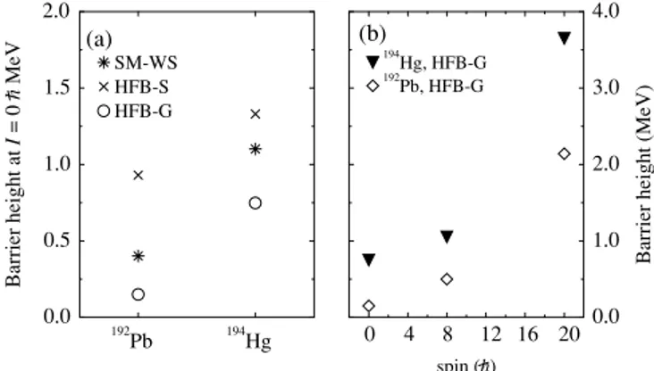
FIG. 4. (a) Comparison of various model predictions of the height of the barrier separating the SD and ND wells in192Pb and194Hg:
Strutinsky method with Woods-Saxon potential (SM-WS) [19], mean field using the Skyrme interaction (HFB-S) [20], and mean field using a Gogny interaction (HFB-G) [21]. (b) Comparison of the barrier heights predicted using the HFB method and a Gogny force for192Pb
and194Hg at various different spins.
Hartree-Fock-Bogoliubov (HFB) [20] methods; more recent HFB calculations [21] have predicted barrier heights for these two nuclei at spinsI =0 ¯h,8 ¯h, and 20 ¯h. The results of these calculations are shown in Fig. 4. All three methods predict that the barrier height for194Hg is larger than for192Pb at spin zero, and the predictions at nonzero spin suggest that the difference remains large and indeed increases towards high spins.
Information concerning relative barrier heights and the stability of the SD well in different nuclei is one of the pri-mary goals of studies of superdeformation. Without knowing whether the mixing is completely statistical or predominantly with one ND level, or the degree to which it is affected by the microscopic structure of the ND states, quantitative comparisons between data and model predictions cannot be made. The problem is analogous to that of pinpointing the reaction mechanism in scattering. If an oversimplified or inappropriate reaction mechanism is assumed, the nuclear structure information obtained will be inconclusive.
III. APPLICATION OF THE MODELS TO THE EXISTING DATA: SPREADING WIDTH RESULTS
Before the three models of the decay described in the previous section can be applied to analyze SD decay profiles, values ofD, ŴN, ŴS, and Iare needed. In the following, we
briefly describe how the values used in this work have been arrived at.
Estimates ofDare usually made using a Fermi gas density of states. The decay widths of the ND states ŴN can be
TABLE I. Values of ND level densities, ND and SDγ-decay widths, and in-band intensity fractions for two levels in the yrast SD bands in192,194Hg and192,194Pb.
Isotope Spin (¯h) D(eV) ŴN(µeV) ŴS(µeV) I
192Hg 10 89 733 50 0.08 192Hg 12 135 613 128 0.74 194Hg 10 14 1487 33 0.05 194Hg 12 19 1345 86 0.60
192Pb 8 1681 169 16 0.25
192Pb 10 1410 188 48 0
.12
194Pb 6 333 405 3 0.04
194Pb 8 273 445 14 0
.65
the quasicontinuum component of the SD decay spectrum has provided a somewhat less precise measurement in192Hg [16]. In this paper, we consider all fiveK=0 “vacuum” bands in the even-even isotopes.
The estimates of D and ŴN also rely on an assumed
“backshift parameter,” which corresponds to the gap in the level density above the yrast line in even-even nuclei due to pairing correlations. In the following, the usual value of the backshift parameter (1.4 MeV) is adopted in the treatment of 192,4Hg, while the spin-dependent backshift parameters suggested in Ref. [23] are adopted in the treatment of192,4Pb. However, it should be noted that these values have uncertainties such that they may increase or decrease by a factor of 2 or more [10,23].
Values ofŴScan be extracted from the data with relatively
small uncertainty (of the order of 10%) if lifetime measure-ments have been made and quadrupole momeasure-ments extracted: such measurements have been made for all of the nuclei considered here [24–27]. The final parameter needed to allow a spreading width to be extracted isI, the fraction of intensity that remains in the SD band. In general, with the high statistics experiments which have been performed in recent years, this is measured to an accuracy of ∼2% of the maximum in-band intensity. The values adopted here are taken from Refs. [5,9,18]. Table I listsD, ŴN, ŴS, andI for two levels
from which significant flux is lost in the yrast SD bands in 192,194Hg and192,194Pb.
Spreading widths extracted using the GW, SH, and SB approaches are listed in Table II. Equivalent calculations for the spin 26¯hand spin 28¯hlevels in152Dy are included in Table II: the values ofD, ŴN, ŴS, andIfor these states are those given in
Ref. [22]. The standard deviations in the in-band SD intensity calculated within the SH model are included in the rightmost column. The small values obtained indicate that, within its range of validity, the model predicts well defined values ofI.
Before discussing the results in detail, we should briefly comment on the fact that, for some levels, the value extracted forŴ↓SBis negative. As previously noted [14,23], the necessity that the spreading width be positive imposes the additional constraint thatŴN > ŴS(I−1−1) in this model. In order to
obtain a positive value for Ŵ↓SB for the anomalous states in 192Pb and 152Dy, the ND γ-decay width would need to be increased by only a factor of 2−3. Given the uncertainties and assumptions employed in estimating D and ŴN, such
an increase is not inconceivable. The negative values should therefore not be taken as an indication of the failure of the model.
IV. COMPARISON OF THE SPREADING WIDTHS AND DISCUSSION
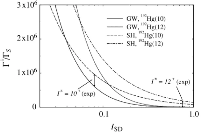
Figure 5 compares the models of GW and SH forŴN/D
equal to the estimated ratios for the two SD levels in 192Hg. The curves illustrate the dependence of the calculated ratio
Ŵ↓/ ŴS as a function of I. For in-band intensities in the
range 0.03−0.1, the values obtained with SH are within an order of magnitude of those obtained with GW. However, for higher intensities, the values obtained with GW drop much more rapidly and the difference between the two approaches becomes several orders of magnitude. Thus, although GW and SH are essentially equivalent in the overlapping resonance region, SH deviates from GW forŴN/D≪1 andI0.1.
It has been suggested that the GW fit formula is accurate to within about 20% for nuclei withA≈190 [9]; SH is valid over a significantly smaller range ofŴN/D. In the cases considered
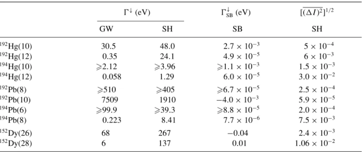
TABLE II. Spreading widths of SD levels in192,4Hg,192,4Pb, and152Dy calculated using the GW, SH, and
SB models. The final column gives the standard deviation calculated using the SH approach.
Ŵ↓(eV) Ŵ↓
SB(eV) [(I)2] 1/2
GW SH SB SH
192Hg(10) 30.5 48.0 2.7
×10−3 5 ×10⁻⁴
192Hg(12) 0.35 24.1 4.9×10⁻⁵ 6×10⁻³
194Hg(10) 2.12 3.96 1.1×10⁻³ 1.5×10⁻³
194Hg(12) 0
.058 1.29 6.0×10⁻⁵ 3
.0×10−2
192Pb(8) 510 405 6
.7×10−5 2
.5×10−4
192Pb(10) 7509 1910 −4.0×10⁻³ 5.9×10⁻⁵
194Pb(6) 99.9 39.3 8.8
×10−5 2.0 ×10⁻⁴
194Pb(8) 0.223 8.41 7.7×10⁻⁶ 7.5×10⁻³
152Dy(26) 68 267 −0.04 2.4×10⁻³
0.1 1.0
ISD
1 x10⁶
2 x10⁶ 3 x10⁶
0
GW, 192Hg(10) GW, 192Hg(12) SH, 192Hg(10) SH, 192Hg(12)
Iπ = 12 +(exp)
Iπ = 10 + (exp)
Γ
/
ΓS ←
FIG. 5. Values of the ratioŴ↓/ Ŵ
S as a function of the in-band
intensityIcalculated forŴN/Dappropriate for the 10+and 12+levels
in192Hg.
here (which are typical of superdeformed bands in theA≈190 and A≈150 regions),ŴN/D≪1 and thus SH should not
be expected to provide a precise model. However, in most cases, the values of Ŵ↓ are comparable (within one or two
orders of magnitude) between the two models. They thus yield comparable values for the mean interaction strength, since both models relateŴ↓andVthrough Eq. (3).
The values ofŴSB↓ , on the other hand, are several orders of magnitude smaller than Ŵ↓ in all cases. Similar differences
were found in Refs. [9,14]. For the Hg and Pb isotopes,
Ŵ↓SB/ Ŵ↓ is in the range 10−3−10−6. The values of Ŵ↓
SB obtained for the two levels in152Dy are also significantly less than Ŵ↓. As noted above, these differences have previously
been dismissed as unimportant because the interaction energies extracted in the two types of model have been found to be similar. In the following, we consider reasons why this attitude may gloss over basic differences in the models.
First, finding the correct value of the spreading width should help us understand its physical significance. The values ofŴSB↓
are very small, and in fact those extracted for the Pb isotopes approach the experimental value of the weak interaction spreading width ŴW=1.8×10⁻⁷ eV obtained in parity
violation studies with epithermal neutrons [28]. The spreading width for decay out of an SD band describes a rearrangement of nucleons due to the strong and electromagnetic interactions. It might therefore be expected to be of similar magnitude
TABLE III. Tunneling widths for escape from the SD well extracted using Eq. (9) and the barrier heights predicted in Ref. [21].
Isotope Spin Ŵtunnel(eV)
194Hg 0 37
194Hg 8 1.6
194Hg 12 (interpolated) 0
.38
194Hg 20 2.4×10⁻¹²
192Pb 0 1.98×10⁴
192Pb 8 508
192Pb 10 (interpolated) 30
192Pb 20 1.77×10⁻⁵
to the spreading widths encountered in other nuclear and electromagnetic processes, i.e., of the order of MeV and eV, respectively. The spreading widths obtained with GW are of this order. The drastic nature of the nuclear shape change may indeed result in a smaller spreading width than is encountered in other strong/EM processes, but the extreme smallness of
ŴSB↓ needs to be understood if the SB model is put forward as an appropriate description of the SD decay and ifŴSB↓ is truly a spreading width.
Second, there is the issue of the relation between the spreading width and the tunneling rate, and by extension, the relation with the size of the barrier separating the SD and ND minima.
If the mixing is statistical and there is a quasicontinuum of ND states, it may be possible to relate the height of the barrier to a fusion-like tunneling rate. Assuming that the barrier and the two wells can be modeled with parabolic and inverse parabolic shapes, the barrier heightBcan be related to a tunneling rate
Ŵtunnelby the relation [9,29]
Ŵtunnel= ¯
hωs
2πe
(−2πB
¯hωb), (9)
where ωs and ωb specify the curvatures of the parabolas
describing the SD well and the barrier, respectively. Making the further assumption that ¯hωs =¯hωb=0.6 MeV [9], it is
possible to use the barrier heights predicted by the Strutinsky or HFB calculations to predict tunneling rates.
As an illustration, we focus on the two nuclei with the lowest and highest measured SD excitation energies,192Pb and194Hg. In both cases, the decay out of the SD band occurs in the spin rangeI ≈14¯h→I ≈8¯h. Barrier height predictions at spins
I =8¯handI =20¯hhave been made for both of these nuclei using the HFB method with a Gogny force [21]. The results of these calculations [shown in Fig. 4(b)] have been used to estimate tunneling widths as described above. The resulting tunneling widths are given in Table III.
The tunneling width associated with the predicted barrier height at spin I =8¯h is close to the lower limit of the spreading width extracted using the two statistical models, and it is several orders of magnitude larger than the lower limits extracted using the two-level mixing model. However, in the limit of mixing with only a small number of ND levels, the relationship between barrier height and tunneling width given in Eq. (9) is not appropriate [30].
In order to compare the tunneling rate with the spreading width of GW for levels where definite values ofŴ↓ andŴ↓
SB are obtained, we have estimated barrier heights atI =12¯hand 10¯h in194Hg and 192Pb, respectively. Using a simple linear interpolation betweenI =8¯handI =20¯h, we obtainB(I = 12¯h,194Hg)=1.98 MeV andB(I =12¯h,192Pb)=0.77 MeV. The tunneling widths corresponding to these values are included in Table III. For 194Hg, Ŵ↓ obtained with GW is
an order of magnitude smaller than the estimated tunneling width (ŴSB↓ is four orders of magnitude smaller); for192Pb, it is two orders of magnitude larger (comparison withŴSB↓ , which is negative in this instance, is not possible).
between the SD and ND states. If the coupling between SD and ND levels is fully statistical, Ŵ↓ and the expression
for Ŵtunnel are meaningful. However, the relatively low ND level density in the two Pb isotopes (where the overlapping resonance region and chaos are not approached) indicates that a fully statistical treatment may not be appropriate. If this is the case, the systematics of the SD minima in theA≈190 region cannot be studied without further theoretical development of the decay-out models.
Finally, we consider whether the similarity of the interaction energies obtained in previous work [9,10] should be considered natural, or even desirable. As illustrated in Fig. 3, the interactionsVandVare not the same, and there is therefore noa priorireason why they should have the same value. In the GW (and SH) approach,Vdescribes the averaged interaction of the SD state with many ND states. In contrast, in the SB approach, V is the interaction between the SD state and a single ND state. Because of these different physical meanings, VandVdepend on different parameters. WhileVandŴ↓
depend on the ND level spacingD,V(but notŴSB↓ ) depends on, the energy difference between the SD state and the ND state it mixes with.
For any real decaying SD level, is unknown, and the resulting interaction strength depends strongly on the value adopted. As an example, the GW approach yieldsV ≈20 eV for the 10+ level in 192Hg: the SB approach yields V ≈ 0.03 eV for =0, but any higher value can be obtained, including 20 eV if≈1.2D. In previous work [9,23], the average SD-ND energy difference=D/4 has been adopted, resulting in V of similar size to V. However, there is no obvious reason to expect that use of the average separation should produce the same effect as averaging the coupling to many ND states. In effect, the GW/SH models offer a means of experimentally determiningVandŴ↓, whereas SB offers
a means of experimentally determiningŴ↓SBbut notV, unless
can be measured (or calculated). The dependence ofIavon
is investigated for a related model in Ref. [31].
The underlying differences between the two types of model are exemplified by the different treatments of the in-band intensity as comprising either one or two contributions. In the analyses using the GW and SH models,Iavis found to be extremely small, andIfldominates. In the SB model, there is no separate fluctuating contribution, and the total intensity is given by Eq. (7). However, in the limit whereŴN ≫Ŵ
↓
SB, this reduces toI →(1+ŴSB↓ / ŴS)−1, which isformallyidentical
to Iav. The data gathered to date suggest that this limit is approached in most physically realized cases.
The motivation behind the SB model may be thought of as similar to the calculation of a “doorway-doorway” interaction in the GW/SH approach, for which a fluctuation contribution could also be calculated [8]. It seems unlikely, given the relatively low ND level density, that a fully statistical mixing process occurs in the decay of SD192Pb, and thus this type of doorway approach may be more suitable than the present statistical models. In addition, the idea of a doorway state, which would have larger overlap with an SD state than other nearby ND states, goes some way towards making allowance for the possible influence of the microscopic structure of the
ND states on the decay. If there are indeed ND doorway states then these in turn will have a spreading widthŴd↓and a
γ-emission (escape) widthŴd, analogous toŴ↓andŴSfor the
in-band SD state. The ND compound widthŴN would then
be reduced (due to flux conservation) to an extent which is measured by an additional parameterµ=Ŵd↓/ Ŵd; a similar
picture has been used to describe the decay of giant resonances [32,33]. Note that the spreading widths Ŵ↓ and Ŵ↓
d depend
on the choice of basis in which the partial diagonalizations which define them are carried out. However, without a reliable calculation of µ, its introduction would not be useful in the context of the present paper: analysis of the experimental intraband intensity Iat present permits the determination of a single parameter Ŵ↓. It may be possible to determine µ
from an analysis of the quasicontinuum component of the decay spectrum [34,35], but it is likely that experimentally distinguishingŴN andŴdwill be extremely difficult.
V. CONCLUSION
In this paper, we have examined the structure of three recent models of SD decay and applied these models to the analysis of the decay of states in four SD bands in nuclei with masses
A ≈ 190 and one SD band in 152Dy. These bands are the only yrast SD bands in even-even nuclei for which excitation energies have been measured and are thus the only such cases where quantitative estimates of the normal deformed state properties can be made. This work represents the first time all of the available experimental data have been compared. Two of these models are fully statistical and describe the physical process where an SD state mixes with many ND states that have structures sufficiently complex so as to be equivalent. The other model assumes that the mixing occurs predominantly with only one ND state (the nearest neighbor). Questions as to the nature of this state, whether complex or of well defined microscopic origin, are not addressed by the model.
Since the two types of model represent physically different processes, they should not be expected to result in the same interaction energy—that is, it should not be expected that V of the statistical mixing model be equal to V of the two-level mixing model. We have stressed the point made by the authors of the two-level mixing model [13,14] thatVcannot be extracted from the data without knowledge of the SD-ND energy separation ; in relation to this we have questioned whether the use of the average separation in that model should be expected to be equivalent to the use of the average over many interactions in the statistical model.
Because of the present impossibility of arriving at a definite value of V for the decay from any measured SD level, comparison should be restricted to a directly calculable quantity such as the spreading width. The energy-averaging SH approach results in similar spreading widths to those extracted in the equivalent ensemble-averaging GW approach, but as expected, the SH model fails more quickly than the GW fit formula as ŴN/D→≪1. The results of these
a simple model of the barrier potential and the predictions of HFB calculations. The two-level mixing approach results in far smaller spreading widths, such that some special explanation of their size would be required if this model of the decay is correct.
The different definitions of the spreading widths indicate that they are incompatible quantities. But the question of which is “correct” is intimately related to which type of model is physically more appropriate. This question is particularly important given the similarity of the decay patterns of SD bands over a wide range of excitation energy above yrast, and hence over a variety of different ND level densities. The experimentally determined SD excitation energies are also beginning to indicate that, at least in some cases such as the two Pb isotopes, it is unlikely that the ND states are
truly compound. Thus, it appears that some consideration of the microscopic structure of the ND states may be required, possibly by the introduction of doorway states. Until it is established which model describes the real process of decay out of the SD well, a deeper understanding of what triggers the decay and why the intensity profiles are so similar cannot be achieved.
ACKNOWLEDGMENTS
This work was carried out with support from the Australian Research Council through Grant DP0451780. MSH is partly supported by FAPESP and the CNPq, and both MSH and AJS are supported by the Instituto de Milˆenio de Informac¸˜ao Quˆantica-MCT, all of Brazil.
[1] B. Singh, R. Zywina, and R. B. Firestone, Nucl. Data Sheets97, 241 (2002).
[2] A. N. Wilsonet al., Phys. Rev. C54, 559 (1996). [3] A. Lopez-Martens, Ph.D. thesis, CSNSM-Orsay, 1997. [4] T. L. Khooet al., Phys. Rev. Lett.76, 1583 (1996). [5] A. N. Wilsonet al., Phys. Rev. Lett.90, 142501 (2003). [6] K. Hauschildet al., Phys. Rev. C55, 2819 (1997). [7] D. Rossbach, Ph.D. thesis, Universit¨at Bonn, 2000.
[8] M. S. Hussein, A. J. Sargeant, M. P. Pato, N. Takigawa, and M. Ueda, Prog. Theor. Phys.154, 146 (2004).
[9] R. Kr¨ucken, A. Dewald, P. von Brentano, and H. A. Weidenm¨uller, Phys. Rev. C64, 064316 (2001).
[10] A. N. Wilson, Prog. Theor. Phy. Suppl.154, 138 (2004). [11] J.-z. Gu and H. A. Weidenm¨uller, Nucl. Phys.A660, 197 (1999). [12] A. J. Sargeant, M. S. Hussein, M. P. Pato, and M. Ueda,
Phys. Rev. C66, 064301 (2002).
[13] C. A. Stafford and B. R. Barrett, Phys. Rev. C60, 051305 (1999). [14] D. M. Cardamone, C. A. Stafford, and B. R. Barrett, Phys. Rev.
Lett.91, 102502 (2003).
[15] S. Siemet al., Phys. Rev. C70, 014303 (2004). [16] T. Lauritsenet al., Phys. Rev. C62, 044316 (2000). [17] G. Hackmanet al., Phys. Rev. Lett.79, 4100 (1997). [18] A. Lopez-Martenset al., Phys. Lett.B380, 18 (1996).
[19] W. Satula, S. Cwi´ok, W. Nazarewicz, R. Wyss, and A. Johnson, Nucl. Phys.A529, 289 (1991).
[20] S. J. Krieger, P. Bonche, M. S. Weiss, J. Meyer, H. Flocard, and P.-H. Heenen, Nucl. Phys.A542, 43 (1992).
[21] J. Libert, M. Girod, and J.-P. Delaroche, Phys. Rev. C60, 054301 (1999).
[22] T. Lauritsenet al., Phys. Rev. Lett.88, 042501 (2002). [23] A. N. Wilson and P. M. Davidson, Phys. Rev. C69, 041303(R)
(2004).
[24] B. C. Busseet al., Phys. Rev. C57, 1017(R) (1998). [25] A. Dewaldet al., Phys. Rev. C64, 054309 (2001). [26] U. J. van Severenet al., Phys. Lett.B434, 14 (1998). [27] A. N. Wilsonet al., Nucl. Phys.A748, 12 (2005).
[28] G. E. Mitchell, J. D. Bowman, S. I. Penttil¨a, and E. I. Sharapov, Phys. Rep.354, 157 (2001).
[29] Y. R. Shimizu, E. Vigezzi, T. Døssing, and R. A. Broglia, Nucl. Phys.A557, 99c (1993).
[30] S. Bjørnholm and J. E. Lynn, Rev. Mod. Phys. 52, 725 (1980).
[31] A. J. Sargeant, M. S. Hussein, M. P. Pato, N. Takigawa, and M. Ueda, Phys. Rev. C69, 067301 (2004).
[32] H. Dias, M. S. Hussein, and S. K. Adhikari, Phys. Rev. Lett.57, 1998 (1986).
[33] V. V. Solokov and V. Zelevinsky, Phys. Rev. C 56, 311 (1997).
[34] S. Åberg, Phys. Rev. Lett.82, 299 (1999).