TUTORIAL FOR MIXTURE-PROCESS EXPERIMENTS WITH AN INDUSTRIAL APPLICATION
Luiz Henrique Abreu Dal Bello
1and Antonio Fernando de Castro Vieira
2*Received December 3, 2009 / Accepted April 1, 2011
ABSTRACT.This article presents a tutorial on mixture-process experiments and a case study of a chemical compound used in the delay mechanism for starting a rocket engine. The compound consists in a three-component mixture. Besides the mixture three-components, two process variables are considered. For the model selection, the use of an information criterion showed to be efficient in the case under study. A linear regres-sion model was fitted. Through the developed model, the optimal proportions of the mixture components and the levels of the process variables were determined.
Keywords: mixture experiments, process variable, linear regression, information criterion, optimization.
1 INTRODUCTION
Formulations of Mixture Experiments (ME) are commonly found in chemical, pharmaceutical and food industries, as well as in other industrial segments. In those experiments, the factors are proportions of the components in a mixture and the response is a variable that characterizes the quality of the product, assumed as a function of component proportion. In those experiments, the sum of component proportions always equals to one. In certain situations, there may be other factors, in addition to the mixture components, that affect the characteristics of the mixture. Such factors are named process variables, which are frequently included in the experiment as factorial designs. Therefore, we intend to determine not only the optimal proportions of the mixture components, but also the optimal levels of the process variables. The aim of this article is to provide a tutorial on Mixture-Process Experiments (MPE).
A chemical mix experiment will be presented, as part of a subsystem of a mechanism to delay the activation of a rocket engine, described in Vieira & Dal Bello (2006) and Dal Bello & Vieira (2008). The aim of the experiment is to find the ideal formulation, so that the expected burning time value is according to the design’s specification, that is, 8 seconds. Such time is optimal for
*Corresponding author
1Centro Tecnol´ogico do Ex´ercito (CTEx), Rio de Janeiro, RJ, Brasil. E-mail: [email protected]
the rocket’s range. As it will be seen, several formulations lead to a time of 8 seconds, being thus convenient to find a formulation that provides the lowest variance for future responses. The mixture components are Zarfesil, Ground Glass and Nitrocellulose. In addition to these mixture variables, other two variables that may also affect the characteristics of the mixture were also taken into consideration. The first is the granulometry of the mixture; the second variable consists of the insertion – or not – of an orifice for gas escape during the burn reaction, making this reaction always to occur at a pressure which is approximately the atmospheric pressure.
2 LITERATURE REVIEW
Cornell (2002) is the main reference on ME, being the Chapter 7 dedicated to MPE cases. In it, a comprehensive and detailed exposition can be found. Myers & Montgomery (2002) dedicate Chapters 12 and 13 to ME and MPE, thus comprising a good introduction to the topic. Piepel (2004) summarizes a survey related to mixture experiments for a period of 50 years, ranging from 1955 to 2004. Prescottet al. (2002) propose a quadratic model as an alternative to the models traditionally used in ME (Scheff´e models). Cornell (2000), Cornell (2002, Chapter 6), Cornell & Gorman (2003) and Khuri (2005) carried out comparative studies between models that they named as slack-variable models and Scheff´e models. Piepel (2007) compares the CSLM (Com-ponent Slope Linear Model) with the SLM (Scheff´e Linear Model) and the CLM (Cox Linear Model). They conclude that the models SLM, CLM and CSLM are mathematically equivalent and provide the same statistics for a given ME. The differences lie in the interpretations of their coefficients.
Goos & Donev (2006) describe an algorithm to plan experiments in blocks involving mixtures. They show that, for restricted and unrestricted experimental regions, the resulting design of ex-periments is statistically more efficient than the options of exex-periments in blocks presented in the literature. Goos & Donev (2007) describe an algorithm to plan split-plot experiments in cases involving mixture and process variables. They use an optimization criterion for the choice of ex-perimental points and show that it is preferable to spread the replications all over the experiment region, instead of concentrating them in central points.
Kowalski et al.(2002), Prescott (2004) and Sahni et al.(2009) analyzed the MPE modeling. Goldfarbet al. (2004a) propose the use of a plot method (variance dispersion plot) for MPE planning. The variance dispersion plot presents a visual way of assessing the variance properties of an MPE within the joint mixture and process area. That information may be used to select experiments with an acceptable variance profile.
3 MIXTURE EXPERIMENTS
Considerxi, the variables that represent the proportions of theqmixture components. Then:
q X
i=1
xi =1; xi ≥0; i=1, . . . , q (1)
The restrictions presented in Equation (1) are shown in Figure 1, in the event of a mixture of two and three components.
2
1 1
1
0
1 + 2 = 1
2
1 1
0 1
1 + 2 + 3 = 1
3
1
a) b)
Figure 1– Restricted factor space for mixtures with a) 2 components and b) 3 components.
The feasible region of the two-component mixture is represented by a line segment and, in case of a three-component mix, it is represented by a triangle. Generally, in case of three-component mixtures, the restricted experimental region is represented by using a 3-coordinate system, as shown in Figure 2. Each edge of the triangle corresponds to a binary mixture, and the vertices of the triangle correspond to the formulations with pure components. The possible ternary mixtures are located inside the triangle. In this case, only two dimensions are needed to represent the experiment. As each component is represented by a vertex, a geometric figure with three apexes and two dimensions – that is, an equilateral triangle – represents the restricted factor space of a ternary mixture.
In many ME there are limitations in the component proportion, making the experimental space a sub-region of the original space. Therefore, upper and/or lower limits are established in the proportions, represented as follows:
0≤Li ≤xi ≤Ui ≤1; i =1, . . . , q (2)
Figure 3 shows an experimental case with a three-component mixture with lower constraints in the proportions of the three components, and a case with four components with upper constraint in the proportion of only one component.
2 3
1
0.4
0.4 0.4
0.6
0.2
0.6 0.6
0.8
0.8
0.2 0.2
0.8
Figure 2– 3-Coordinate System.
x2 x3
L1
L2
L3
x1
x2 = 1
x3 = 1
x1 = 1
x4 = 1
C F
B
A
D
E G
U1
a) b)
Figure 3– a) lower and b) upper constraints in the proportion of components.
We then have two types of pseudocomponents: the L-pseudocomponents in relation to the lower limit, and the U-pseudocomponents in relation to the upper limit. According to Cornell (2002, p. 134), the main reason to use pseudocomponents is that it is usually easier to plan the experi-ment and fit the model. Myers & Montgomery (2002, p. 655) recommend the use of pseudocom-ponents to fit mixture models where there are component constraints, resulting in mild to high levels of multicollinearity. Generally speaking, a mixture model that uses pseudocomponents will have lower levels of multicollinearity than the same model with the original components.
The L-pseudocomponents are defined as:
vi =
xi−Li
1−L ; i =1, 2, . . . , q (3)
whereL=Pq i=1Li.
In order to obtain original components(xi), just use the Equation (3):
xi =Li +(1−L) vi (4)
The U-pseudocomponents are defined as:
ui =
Ui−xi
U−1 , i=1, 2, . . . , q (5)
whereU= q P
i=1 Ui.
In order to calculate respective original components(xi), just use the Equation (5):
xi =Ui−(U−1)ui (6)
Where there are upper and lower constraints simultaneously, the choice of using L-pseudo-components, vi, or U-pseudocomponents, ui, depends on the shape of the experimental
re-gion. Where(1−L) < (U−1), the choice if for L-pseudocomponents, and where(1−L)≥
(U−1), the choice is for U-pseudocomponents (Cornell, 2002, p. 160).
4 MODEL FOR MIXTURE-PROCESS EXPERIMENTS
4.1 Models for Mixture Experiments
The models which are traditionally used in mixture experiments are Scheff´e’s canonical polyno-mials (Cornell, 2002). Scheff´e’s Quadratic Model is as follows:
Q(β, x)= q X
i=1 βixi+
X q X
i<j
βi jxixj (7)
Scheff´e’s Cubic Model is as follows:
C(β, =x) = q X
i=1 βixi+
X q X
i<j
βi jxixj+ X X
q X
i<j<k
βi j kxixjxk
+ X
q X
i<j
βi−jxixj xi−xj
(8)
Scheff´e’s Special Cubic Model is the same as the Cubic Model, excluding the terms
X q X
i<j
βi−jxixj xi −xj.
For the cases where there are high levels of multicollinearity, the use of slack-variable models is recommended (Cornell, 2002, Chapter 6). In a mixture of q components, being aware of the proportion of the first(q −1)components, it is possible to determine also the proportion of componentq, since xq = 1−x1−x2− ∙ ∙ ∙ −xq−1. Therefore, xq is defined as the slack
variable, which will not be part of the composition of the model terms. In order to balance out the lack of the slack variable, an intercept is included to the model. Therefore, for a mixture of q components there areq possibilities of slack variables, that is,q different models with slack variable.
The Quadratic Model with slack variable:
Q(β, x)=β0+ q−1 X
i=1 βixi+
X q−1 X
i≤j
βi jxixj (9)
The Cubic Model with slack variable:
C(β, x)=β0+ q−1 X
i=1 βixi+
X q−1 X
i≤j
βi jxixj+ X
q−1 X
i≤j≤k X
βi j kxixjxk (10)
4.2 Model for Process Variables
An adequate model forr process variablesz1,z2, . . . ,zr, involving second-order terms is
(Cor-nell, 2002):
Q(α, z)=α0+ r X
l=1 αlzl+
r X
l=1 αllzl2+
X r X
l<m
αlmzlzm (11)
4.3 Mixture Model Including Process Variables
The experimental design is established through a combination of the mixture variables with the process variables. In addition, any model for the mixture may be combined with the model for the process variables, in order to represent mixture-process-type problems. Consider f(x)the for the mix andg(z)the model for the process variables. Then, the additive model combined for the mixture-process case is (Prescott, 2004)
C(x,z)= f(x)+g(z) (12)
For example, the additive combined model, which includes Scheff´e’s cubic model for the mixture presented in Equation (8) and the reduced quadratic model, considering only the main effects of the process variables and the
C(γ, x, z) = q X
i=1 γi0xi+
X q X
i<j
γi j0xixj+ X X
q X
i<j<k
γi j k0 xixjxk
+ X
q X
i<j
γi0−jxixj xi−xj+ r X
l=1 γ0lzl+
X r X
l<m
γ0lmzlzm
(13)
where theγ’s are the parameters for the mixture’s combined model including process variables. The lower indexes ofγrefer to mixture variables, whereas the upper ones refer to process vari-ables. Observe that the combined model presented in Equation (13) does not have the intercept originated from the model for the process variables. The intercept is eliminated from the com-bined model, since it has a linear dependence with the termsγi0x, due to the constraint presented in Equation (1). Those additive models do not take into account the effects of process variables on the linear and non-linear properties of the mixture components. Alternative models were suggested, with the introduction “crossed” terms in f(x)and g(z). The complete cross-over model is
C(x,z)= f(x)×g(z) (14)
The combined multiplicative model that includes Scheff´e’s cubic model for mixtures and the re-duced quadratic model for the process variables. This combined model is represented as follows:
C(γ,x,z) = q X
i=1 γi0xi+
X q X
i<j
γi j0xixj + X X
q X
i<j<k
γi j k0 xixjxk
+ r X l=1 q X i=1 γilxi+
X q X
i<j
γi jlxixj+ X X
q X
i<j<k
γl
i j kxixjxk
zl
+ r X
l<m
q X
i=1
γilmxi+ X
q X
i<j
γi jlmxixj+ X X
q X
i<j<k
γi j klmxixjxk
zlzm
However, the combined models that include the additive and multiplicative model terms simul-taneously may also be considered.
5 D-OPTIMAL DESIGN OF EXPERIMENTS
When there are constraints in the proportions of the mixture components, the use of experiments generated according to some optimization criterion is recommended (Cornell, 2002, p. 400). Cornell (2002) describes four alphabetic optimization criteria (A-optimal, D-optimal, G-optimal and V-optimal) for the choice of the experimental points. Such criteria are based on the opti-mization of some information matrix function W′W, whereWis a matrix (n× p), whose elements are the proportions of the mixture components(xi), the levels of the process variables
(zi)and thexi andzi functions (such as interactions), wherenis the number of observations in
the experiment and pis the number of model parameters. The general combined mixture model with inclusion of process variables is represented in matrix form:
y=Wβ+ε (16)
Fornobservations,yis a vector(n×1)of the observations,βis a vector(p×1)of the coefficients andεis a vector (n ×1)of the random errors. In the classical linear regression model, εis considered with multivariate normal distribution, that is,ε∼N 0,Iσ2.
The estimation vector for the coefficients isβˆ = W′W−1W′y, the variance-covariance matrix is var(β)ˆ =σ2 W′W−1. The prediction value for the response at pointw(w′is a matrix line W) isyˆ(w)and its variance is
varyˆ(w)=σ2w′ W′W−1w (17)
The statistical software Design-Expertr, developed and distributed by the company Stat-Ease, uses the D-optimal criterion for the choice of the experimental points. Myers & Montgomery (2002) define the D-optimal criterion using the moment matrix M=W′W/n. According to these authors, a D-optimal experiment is the one that makes the determinant of the moment matrix, |M|, to be maximized. They show that the determinant of the moment matrix has the following property:
|M| =
W′W
np (18)
With all that, and assuming that the error are normally distributed, independent and with con-stant variance the determinant W′W is inversely proportional to the squared volume of the confidence region on the regression coefficients. WhenW′Wis small, it means that the inverse ofW′Wis large and, therefore, the volume of the confidence region is large; thus, the estimated βis not regarded as good (Myers & Montgomery, 2002, Appendix 7).
6 DELAY MIX EXPERIMENT
The chemical mix under study is part of a subsystem of a mechanism to delay the ignition of a rocket engine, which evolved from the R&D stage in laboratory scale to be currently produced at industrial scale. The aim of the experiment is to find the ideal formulation, so that the expected burning time value is according to the project’s specification, that is, 8 seconds. Such time is optimal for the maximization of the rocket’s range. As it will be seen, several formulations lead to a time of 8 seconds, being thus convenient to find a formulation that provides the lowest variance for future responses.
The mixture components are Zarfesil(x1), Ground Glass(x2)and Nitrocellulose(x3), with the following limitations in the proportions: 0.77 ≤ x1 ≤ 0.81, 0.14 ≤ x2 ≤ 0.18 and 0.05 ≤ x3≤0.07.
As presented in Section 3, where there are simultaneous upper and lower constraints in the mixture components proportions, the L-pseudocomponents are chosen if(1−L) < (U−1). In the case concerned, the choice was for the L-pseudocomponents, as (1−L) = 0.04 and (U−1)=0.06.
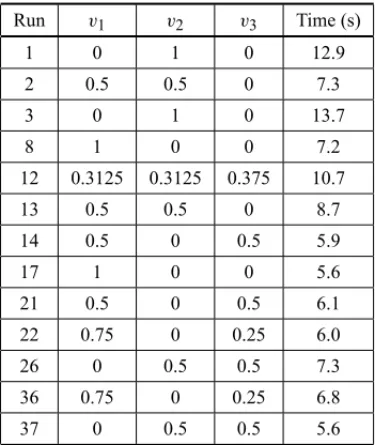
Table 1 shows the experimental design of the delay mix, as well as the experiments’ responses.
Table 1– Reduced experiment of D-Optimal delay mix with L-pseudocomponents. Run v1 v2 v3 Time (s)
1 0 1 0 12.9
2 0.5 0.5 0 7.3
3 0 1 0 13.7
8 1 0 0 7.2
12 0.3125 0.3125 0.375 10.7 13 0.5 0.5 0 8.7 14 0.5 0 0.5 5.9
17 1 0 0 5.6
21 0.5 0 0.5 6.1 22 0.75 0 0.25 6.0 26 0 0.5 0.5 7.3 36 0.75 0 0.25 6.8 37 0 0.5 0.5 5.6
Considering the figures presented in Table 1 and using the backward method, the following Scheff´e model is obtained:
ˆ
Now, considering the terms from slack variable modelsv1,v2andv3and the backward method, the following models are obtained, respectively:
ˆ
y=6,47−0,70v2−0,80v3+99,06v2v3+7,53v22−207,32v22v3 (20)
ˆ
y=13,30−14,30v1+10,93v3+58,11v1v3+7,40v21−49,26v 2
3−77,42v 2
1v3 (21)
ˆ
y=5,67+0,80v1−4,50v2+128,99v1v2+12,13v22−248,79v21v2 (22)
6.1 Delay Mix Experiment with Process Variables
In addition to the mixture variables, other two variables that may also affect the characteristics of the mixture were also taken into consideration. The first one is the granulometry(z1), which may be regarded as a categorical process variable, and will be varied at two levels. The granu-lometry currently used in the production of the delay mix is the 20-30 (level[−1]); however, the granulometry 25-30 (level [1]) is believed to provide a reduction in the variability of the burning times. The second variable(z2)may be regarded as a design variable, as it is a modification of the original delay mechanism design. The insertion of an orifice for gas exhaustion during the burn reaction was suggested, making this reaction always to occur at a pressure which is approximately the atmospheric pressure. Currently, the burning reaction occurs in a confined environment, at a pressure under transient conditions. The insertion of an orifice for gas escape is expected to contribute to the reduction of response variability. That design variable may be seen as a categorical process variable, which will also be experimented in two levels (without orifice[−1]and with orifice [1]). Therefore, the problem of the delay mix may be addressed as a mixture experiment with three components, including two category process variables, which may be represented aszl = −1,1;l=1, 2.
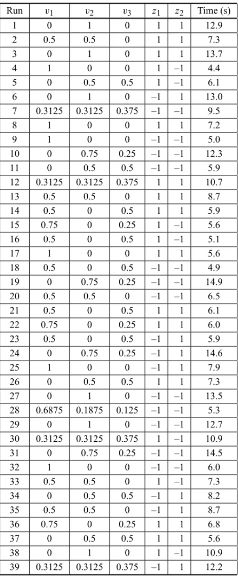
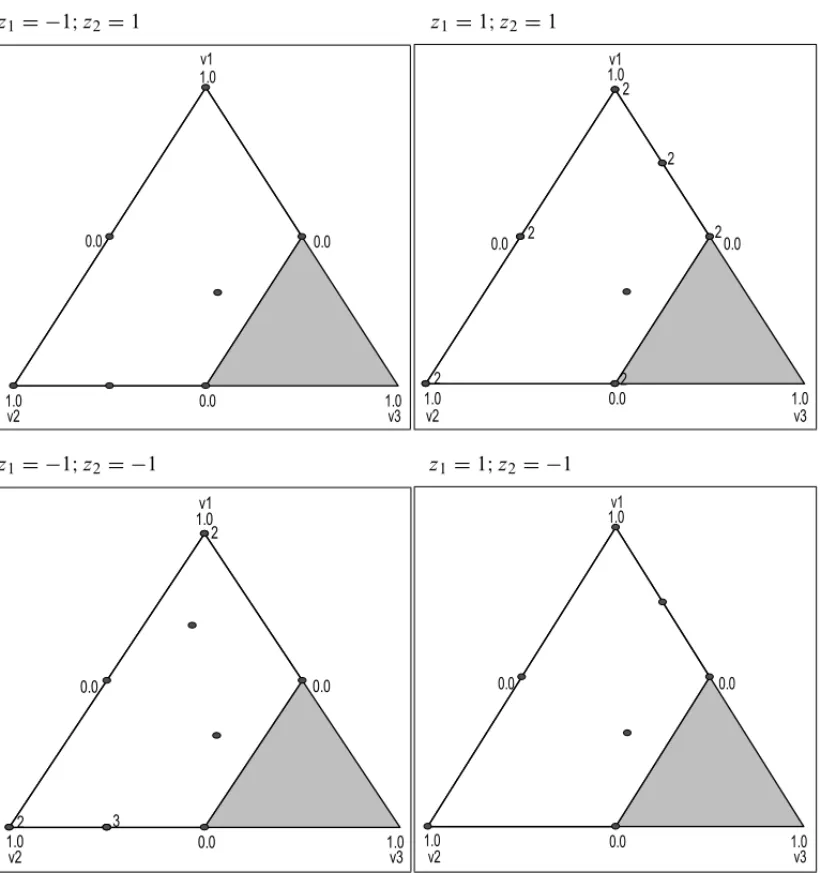
With the constraints in the mixture components, the resulting experimental region becomes a sub-region of the original experimental space. Under such conditions, Cornell (2002) recommends the use of some computer algorithm for the choice of experimental points according to some optimization criterion, arising out of some previously selected candidate points. The software Design-Expertr 7 offers the option of planning restricted mixture experiments in the propor-tions of the components and including process variables. For the choice of experimental points arising out of some previously selected candidate points, the software uses the D-optimal crite-rion, which was presented in Section 5. For the delay mix problem, Design-Expertrgenerated a D-Optimal experiment according to Table 2 and Figure 4, which also presented the results obtained in the random execution sequence in which the experiments were performed.
Table 2– Experiment of D-Optimal delay mix with L-pseudocomponents. Run v1 v2 v3 z1 z2 Time (s)
1 0 1 0 1 1 12.9
2 0.5 0.5 0 1 1 7.3
3 0 1 0 1 1 13.7
4 1 0 0 1 –1 4.4
5 0 0.5 0.5 1 –1 6.1
6 0 1 0 –1 1 13.0
7 0.3125 0.3125 0.375 –1 –1 9.5
8 1 0 0 1 1 7.2
9 1 0 0 –1 –1 5.0
10 0 0.75 0.25 –1 –1 12.3 11 0 0.5 0.5 –1 –1 5.9 12 0.3125 0.3125 0.375 1 1 10.7
13 0.5 0.5 0 1 1 8.7
14 0.5 0 0.5 1 1 5.9
15 0.75 0 0.25 1 –1 5.6 16 0.5 0 0.5 1 –1 5.1
17 1 0 0 1 1 5.6
18 0.5 0 0.5 –1 –1 4.9 19 0 0.75 0.25 –1 –1 14.9 20 0.5 0.5 0 –1 –1 6.5
21 0.5 0 0.5 1 1 6.1
22 0.75 0 0.25 1 1 6.0 23 0.5 0 0.5 –1 1 5.9 24 0 0.75 0.25 –1 1 14.6
25 1 0 0 –1 1 7.9
26 0 0.5 0.5 1 1 7.3
27 0 1 0 –1 –1 13.5
28 0.6875 0.1875 0.125 –1 –1 5.3
29 0 1 0 –1 –1 12.7
30 0.3125 0.3125 0.375 1 –1 10.9 31 0 0.75 0.25 –1 –1 14.5
32 1 0 0 –1 –1 6.0
33 0.5 0.5 0 1 –1 7.3 34 0 0.5 0.5 –1 1 8.2 35 0.5 0.5 0 –1 1 8.7 36 0.75 0 0.25 1 1 6.8
37 0 0.5 0.5 1 1 5.6
38 0 1 0 1 –1 10.9
z1= −1;z2=1 z1=1;z2=1
z1= −1;z2= −1 z1=1;z2= −1
Figure 4– Experiment of D-Optimal delay mix with L-pseudocomponents.
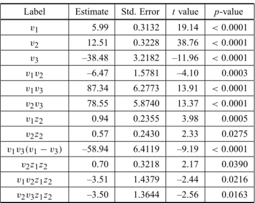
At first, a model using the stepwise, forward or backward model was fitted. The backward method provided a better model than those obtained through the forward and stepwise methods. The following model was fitted with the backward method.
ˆ
y = 5,99v1+12,51v2−38,48v3−6,47v1v2+87,34v1v3 + 78,55v2v3+0,94v1z2+0,57v2z2− 58,94v1v3(v1−v3) + 0,70v2z1z2−3,51v1v2z1z2−3,50v2v3z1z2
(23)
Table 3– M1-Model Test.
Label Estimate Std. Error tvalue p-value v1 5.99 0.3132 19.14 <0.0001 v2 12.51 0.3228 38.76 <0.0001 v3 –38.48 3.2182 –11.96 <0.0001 v1v2 –6.47 1.5781 –4.10 0.0003 v1v3 87.34 6.2773 13.91 <0.0001 v2v3 78.55 5.8740 13.37 <0.0001 v1z2 0.94 0.2355 3.98 0.0005 v2z2 0.57 0.2430 2.33 0.0275 v1v3(v1−v3) –58.94 6.4119 –9.19 <0.0001 v2z1z2 0.70 0.3218 2.17 0.0390 v1v2z1z2 –3.51 1.4379 –2.44 0.0216 v2v3z1z2 –3.50 1.3644 –2.56 0.0163
The lack-of-fit test was not significant, with a p-value of 0.9336.
The ME data modeling may become very complex when the region of definition of the compo-nents is very limited. When the interval of a variable is substantially smaller than the interval of other variables, there may be high level of multicollinearity. This collinearity may turn the estimators of model coefficients unstable and very inflated. In this situation, the model fitting may not be simple, as the columns ofW(covariates matrix) may be nearly linearly dependent. As a result,W′Wmay be nearly singular, and the least-squares estimators of the parameters inβ may have great standard deviations and be highly correlated, besides the fact that the estimates depend on the precise location of the experimental points. In this context, stepwise, forward and backward selection of variables may result in arbitrary selection of variables that belong to the model (Harrell, 2001, p. 64). Therefore, the selection of the “best” model arising out of a set of candidate models may be very complex. One alternative is to use criteria based on the informa-tion theory. Once all the terms that may be part of the MPE model are known, we may then use model selection criteria based on Information Theory.
For model selection, Akaike (1973) developed the Akaike Information Criterion,AIC. However, Burnham & Anderson (2002) recommend the use ofAIC only when n/p ≥ 40, beingn the number of observations and p the number of parameters in the model. For this experiment, n=39. Consequently,AICis not recommendable.
For the selection of models in the event of responses with normal distribution and small samples (n/p<40), Hurvich & Tsai (1989) developed theAICcriterion.
AI Cc=ln
ˆ
σ2p+ n+p
n−p−2 (24)
A Matlabr routine was prepared for the case of delay mix of MPE, for the calculation and storage ofAICvalues. Among all of the models, the one to display the smallestAICcvalue was
chosen (Model M2) (see Dal Bello, 2010 and Dal Bello & Vieira, 2011)
ˆ
y = 6,11v1+5,22v2+32,11v3+ +0,59z2+7,35v22−2,58v2z1z2
−110,24v33−53,48v1v3(v1−v3)+3,31v22z1z2
(25)
Table 4 shows thet-Student test for the Model M2.
Table 4– M2-Model Test.
Label Estimate Std. Error tvalue p-value v1 6.11 0.2564 23.83 <0.0001 v2 5.22 1.1037 4.73 0.0001 v3 32.11 1.7490 18.36 <0.0001 z2 0.59 0.1176 5.06 <0.0001 v22 7.35 1.2196 6.03 <0.0001 v2z1z2 –2.58 0.8205 –3.15 <0.0001 v33 –110.24 7.1329 –15.46 0.0037 v1v3(v1−v3) –53.48 5.7271 –9.34 <0.0001 v22z1z2 3.31 0.9799 3.37 0.0021
The lack-of-fit test was not significant, with a p-value of 0.9775.
As it will be seen below, the Model M2, presented in Equation (25), is better than the Model M1, presented in Equation (23).
Myers & Montgomery (2002) recommend the use of studentized residuals to check the following assumptions: normality, independence and constant variance. The studentized residuals(ri)are
defined as follows:
ri =
ei p
ˆ
σ2(1−hii)
(26)
whereei =yi − ˆyi andhii are elements of the hat matrix diagonalsH=W(W′W)−1W′.
Figures 5 to 8 present the diagnosis plots used to check the adequacy of the fitted model. In the normal probability plot for the studentized residuals shown in Figure 5, we may observe that there is no indication that the normality assumption should not be accepted, as there are no points way off the alignment.
In order to check the independence assumption, there is the studentized residuals plot for the observations in the order in which the experiments were performed (see Fig. 6).
Normal quantiles
S
tu
d
en
ti
ze
d
re
si
d
u
a
ls
-3 -2 -1 0 1 2 3
-3
-2
-1
0
1
2
3
Figure 5– Normal probability plot for the studentized residuals.
Run number
S
tu
d
en
ti
ze
d
re
si
d
u
a
ls
0 10 20 30 40
-3
-2
-1
0
1
2
3
Figure 6– Plot of studentized residuals versus run number.
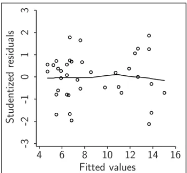
In order to check the additivity of the model regarding the linear model, there is the plot of studentized residualsversusfitted values, shown in Figure 7.
As the residuals shown in the plot from Figure 7 are randomly distributed around zero, there is no reason to suspect that the additivity assumption should not be accepted.
In order to check the assumption of constant variance, the plot of absolute values of studentized residualsversusfitted values, which is shown in Figure 8 is used.
The plot shown in Figure 8 does not present any indication of growth of variance with the increase in the fitted value.
Fitted values
S
tu
d
en
ti
ze
d
re
si
d
u
a
ls
4 6 8 10 12 14 16
-3
-2
-1
0
1
2
3
Figure 7– Plot of studentized residualsversusadjusted value.
Fitted values
A
b
so
lu
te
st
u
d
en
ti
ze
d
re
si
d
u
a
ls
4 6 8 10 12 14 16
0
1
2
3
Figure 8– Plot to check non-homogeneity of variance.
7 RESPONSE OPTIMIZATION
This section presents the response optimization taking Models M1 and M2 into account. We may observe that the Model M2 provides the lowest variance of a future response at the point of interest. As mentioned above, a response of 8 seconds is desirable in the delay mix experiment. Several formulations may result in prediction of new response equal to 8 seconds. Consequently, a desirable aim is to minimize the variance of a new response among the combinations of formu-lations and process variables that result in an expected response value of 8 seconds. Figures 9 to 12 present contour plots of response prediction and standard deviation of the mean response as a function of the L-pseudocomponents and the level of process variables(z1=1 andz2 =1), considering the Models M1 and M2.
v1
1
v2
1
v3
1
0
0
0
77
8 9
10
11 2
2
2
2
2
2
Figure 9– Contour plots of response prediction for Model M1.
v1 1
v2 1
v3 1
0 0
0
7
7 7
8 9
10
11
2
2
2
2
2
2
v1
1
v2
1
v3
1
0
0
0
0.27
0.29 0.31
0.33
0.33 0.33
0.35
0.35
0.35 2
2
2
2
2
2
Figure 11– Contour plots of standard deviation for Model M1.
v1 1
v2 1
v3 1
0 0
0
0.25 0.25
0.27 0.27
0.29 0.29
0.31 0.31
0.33 0.33
2
2
2
2
2
2
the mean near 0.27 (Model M2) and 0.25 (Model M1) must be obtained. However, a stricter optimization procedure must be performed.
The estimation vector for the coefficients isβˆ = W′W−1W′y, the variance-covariance matrix is var(β)ˆ =σ2 W′W−1. The prediction value for the response at pointw(w′is a matrix line W) is represented byyˆ(w)and its variance vary(ˆ w)=σ2w′ W′W−1w. Suppose any given pointw0in the space of the mixture components and the process variables, the model in the point may be represented as follows:y(w0)=w′0β+ε.
The estimation for a new response at this point is the same estimation of the mean:
E ˆ
y(w0)=w′0βˆ (27)
The variance for a new response at this point is then:
varyˆ(w0)=varw′0βˆ +ε
=varw′0βˆ
+var(ε)=σ2w′0(WW)−1w0+σ2 (28)
or:
varyˆ(w0)
=σ2hw′0 W′W
−1
w0+1 i
(29)
The problem may then be formulated as follows:
min var
ˆ
y(w0)=σ2hw′0 W′W −1
w0+1i
subject to: E ˆ
y(w0)=w′0β=8; v1+v2+v3=1; 0≤v1≤1; 0≤v2≤1; 0≤v3≤0,5; z1= −1, 1;
z2= −1, 1.
.
Using a codified search routine in Matlabr, the following solutions were found:
Model M1:
v1=0,5026; v2=0,0855; v3=0,4119; z1=1; z2=1;
var ˆ
y(w0)=0,6626; E ˆ
y(w0)=8,0001. Model M2:
v1=0,4995; v2=0,0652; v3=0,4353; z1=1; z2=1;
var ˆ
y(w0)=0,5757; E ˆ
y(w0)=8,0000.
Model M1:
x1=0,7901; x2=0,1434; x3=0,0665; z1=1; z2=1.
Model M2:
x1=0,7900; x2=0,1426; x3=0,0674; z1=1; z2=1.
By analyzing the solutions, we may conclude that the two models provide practically the same mix formulation at the optimal point. However, the Model M2 is chosen, since it provides better variance (0.5757) for the estimation of future responses.
8 CONCLUSIONS
A tutorial for mixture-process experiments was presented, as well as the mixture experiment with the inclusion of process variables. There is a wide range of combined models to represent the problems of the mixture-process type. In addition, the constraints in mixture experiments are very common, thus making the resulting experimental region a sub-region of the original region.
The data analysis in very restricted mixture regions may be very complex due to the very nature of the mix variables, with possible multicollinearity among some of the terms of the model concerned, which may result in very unstable and inflated coefficient estimators, resulting in arbitrary selection of important variables. With a view to reducing the effect of this type of problem, the use of pseudocomponents was chosen, instead of actual components.
At first, the backward model selection method was used and, then, a model selection method based on the Information Theory, which proved to be more efficient in the case under study.
Then a model was selected, with which was possible to determine the proportion of each of the three components of the chemical mix and the level of the two process variables, so that the prediction of the delay time has minimum variance and expected value of 8 seconds.
It is worth pointing out that the proposed modification of process in relation to the granulometry of the mix and the introduction of the orifice in the delay mechanism result in the reduction of the variance of a new response at the point of interest.
REFERENCES
[1] AKAIKEH. 1973. Information Theory and an Extension of the Maximum Likelihood Principle, in Mehra RK & Csaki F (editors),Second International Symposium on Information Theory. Akademiai Kiado, Budapest.
[2] BURNHAMKP & ANDERSONDR. 2002.Model Selection and Multimodel Inference: A Practical Information-Theoretical Approach. Second edition, Springer, New York.
[3] CHUNGPJ, GOLDFARB HB & MONTGOMERY DC. 2007. Optimal Designs for Mixture-Process Experiments with Control and Noise Variables.Journal of Quality Technology,39: 179–190. [4] CORNELL JA. 2000. Fitting a Slack-Variable Model to Mixture Data: Some Questions Raised.
[5] CORNELLJA. 2002.Experiments with Mixtures: Designs, Models and the Analysis of Mixture Data. 3rdedition, John Wiley & Sons, New York.
[6] CORNELL JA & GORMAN JW. 2003. Two New Mixture Models: Living With Collinearity but Removing its Influence.Journal of Quality Technology,35: 78–88.
[7] DALBELLOLHA. 2010. Modelagem em Experimentos Mistura-Processo para Otimizac¸˜ao de Pro-cessos Industriais. D.Sc. Thesis, Departamento de Engenharia Industrial, Pontif´ıcia Universidade Cat´olica do Rio de Janeiro.
[8] DALBELLO LHA & VIEIRA AFC. 2010. Optimization of a Product Performance Using Mixture Experiments.Journal of Applied Statistics,37: 105–117.
[9] DALBELLOLHA & VIEIRAAFC. 2011 (to be published). Optimization of a Product Performance Using Mixture Experiments Including Process Variables.Journal of Applied Statistics.
[10] GOLDFARBHB, BORRORCM & MONTGOMERYDC. 2003. Mixture-Process Variable Experiments with Noise Variables.Journal of Quality Technology,35: 393–405.
[11] GOLDFARB HB, BORROR CM, MONTGOMERY DC & ANDERSON-COOK CM. 2004a. Three-Dimensional Variance Dispersion Graphics for Mixture-Process Experiments. Journal of Quality Technology,36: 109–124.
[12] GOLDFARBHB, BORRORCM, MONTGOMERYDC & ANDERSON-COOKCM. 2004b. Evaluating Mixture-Process with Control and Noise Variables.Journal of Quality Technology,36: 245–262. [13] GOOSP & DONEVAN. 2006. The D-Optimal Design of Blocked Experiments with Mixture
Com-ponents.Journal of Quality Technology,38: 319–332.
[14] GOOSP & DONEVAN. 2007. Tailor-Made Split-Plot Designs for Mixture and Process Variables. Journal of Quality Technology,39: 326–339.
[15] HARRELLFE JR. 2001.Regression Modelling Strategies With Applications to Linear Models, Logis-tic Regression, and Survival Analysis. Springer-Verlag, New York.
[16] HURVICHCM & TSAIC-L. 1989. Regression and Time Series Model Selection in Small Samples. Biometrika,76: 297–307.
[17] KHURIAI. 2005. Slack Variable Models Versus Scheff´e’s Mixture Models.Journal of Applied Statis-tics,32: 887–908.
[18] KOWALSKISM, CORNELLJA & VININGGG. 2002. Split-Plot Designs and Estimation Methods for Mixture Experiments with Process Variables.Technometrics,44: 72–79.
[19] MYERS RH & MONTGOMERY DC. 2002.Response Surface Methodology: Process and Product Optimization Using Designed Experiments. 2ndedition. John Wiley & Sons, New York.
[20] PIEPEL GF. 2004. 50 Years of Mixture Experiment Research: 1955-2004, in Response Surface Methodology and Related Topics. A.I. Khuri, ed., World Scientific Publishing, Singapore, 283–327.
[21] PIEPELGF. 2007. A Component Slope Linear Model for Mixture Experiments.Quality Technology & Quantitative Management,4(3): 331–343.
[22] PRESCOTTP. 2004. Modeling in Mixture Experiments Including Interactions with Process Variables. Quality Technology & Quantitative Management,1(1): 87–103.
[24] SAHNINS, PIEPELGF & NÆST. 2009. Product and Process Improvement Using Mixture-Process Variable Methods and Optimization Techniques.Journal of Quality Technology,41(2): 181–197. [25] VIEIRAAFC & DALBELLOLHA. 2006. Experimentos com Mistura para Otimizac¸˜ao de Processos: