Mathematical expressions from national codes show that concrete elastic modulus is a function of concrete compressive strength. But concrete, regarded as a three-phase composite material, has elastic properties directly affected by the interfacial transition zone (ITZ), which is character-ized by its higher porosity in comparison to the cement paste. Micromechanical models such as the Mori-Tanaka and three-phase sphere may be applied with good results when used to analyze the concrete. This paper presents a study on the evolution of the concrete elastic modulus, this study is carried out by the application of normative expressions and micromechanics models. Compared to the experimental results, a good itting of micromechanical modeling with ITZ included is observed. Additionally, the quality of the NBR 6118:2003 and CEB-90 expressions is conirmed.
Keywords: concrete, elastic modulus, normative expressions, micromechanic, interfacial transition zone.
Expressões presentes nas normas nacionais e internacionais relacionam o módulo de elasticidade do concreto com a resistência à compressão. O concreto, considerado como material compósito trifásico, tem suas propriedades elásticas diretamente inluenciadas pela zona de transição (ITZ), a qual é caracterizada por sua maior porosidade em relação à pasta de cimento. Modelos de micromecânica como os de Mori-Tanaka e esfera de três fases podem ser aplicados com bons resultados quando utilizados para a análise do concreto. Este trabalho apresenta um estudo sobre o comportamento evolutivo do módulo de elasticidade do concreto, tal estudo é feito mediante a aplicação das expressões normativas e de modelos de micromecânica. Comparado-se com os valores experimentais produzidos percebe-se uma boa concordância quando a modelagem micromecânica leva em conta a ITZ. Também é conirmada a qualidade das expressões da NBR 6118:2003 e do CEB-90.
Palavras-chave: concreto, módulo de elasticidade, expressões normativas, micromecânica, zona de transição.
Contribution to the obtainment of concrete elastic
modulus using micromechanics modeling
Contribuição à obtenção do módulo de elasticidade
do concreto utilizando modelagem micromecânica
A. H. BARBOSA a [email protected]
P. A. LOPEZ-YANEZ b [email protected]
A. M. P. CARNEIRO c [email protected]
a Colegiado de Engenharia Civil, Universidade Federal do Vale do São Francisco, e-mail: [email protected], Av. Antônio Carlos Magalhães, 510, Country Club, Juazeiro-BA, Brasil, CEP 48902-300.
b Departamento de Engenharia Civil, Universidade Federal de Pernambuco, e-mail: [email protected], Av. Acad. Hélio Ramos, s/n – CTG/DECIV, Várzea, Recife-PE, Brasil, CEP 50740-530.
c Departamento de Engenharia Civil, Universidade Federal de Pernambuco, e-mail: [email protected], Av. Acad. Hélio Ramos, s/n – CTG/DECIV, Várzea, Recife-PE, Brasil, CEP 50740-530.
Received: 27 Oct 2010 • Accepted: 03 Sep 2011 • Available Online: 28 Nov 2011
Abstract
1. Introduction
The mechanical properties of the concrete are fundamental in ap-plications of such structural material [1]. Examples are the com-pressive strength and the elastic modulus, which are parameters directly related to the structural design.
In the 49th Brazilian Concrete Congress, carried out in 2007, con-troversial themes were debated, including “Elastic Modulus: Myths and Realities”. Interesting aspects on this important property and the necessity of experimental evaluation were discussed. It was reported that, in general, engineers give to the elastic modulus a secondary role, using the mathematical expression recommended by the Brazilian code (NBR 6118:2003) [2].
According to this code, updated by NBR 6118:2007 code, the elas-tic modulus has to be determined by lab tests according to the NBR 8522:1984 code, update by NBR 8522:2008 [4], and, when lab tests are not conducted, a mathematical expression may be adopted, as a function of concrete compressive strength, yet an age of 28 days is assumed.
International codes such as Eurocode, ACI and CEB-FIP suggest different relationships for determining the concrete elastic modulus, which may be expressed as functions of compressive strength; it is also seen, in some mathematical expressions, that this parameter is related to the concrete density and to the type of aggregate used. Papers such as [5-9] indicate that the concrete elastic modulus is dependent on the cement paste microstructure and on the type of aggregate used. It may be noted that:
n In [5], the inluence of coarse aggregate type on concrete prop-erties was studied, showing a relationship between concrete properties such as compressive strength, elastic modulus and the coarse aggregate source, particularly in the case of quartz. n Analyses carried out by [6] intend to evaluate the probability
that the failure surface occurs throughout the concrete coarse aggregate. In the analysis of fractured sections, the authors found that: when the water/cement ratio is increased, in the case of aggregates with characteristic diameter larger than 16 mm, the rupture probability throughout the aggregates de-creases. It is important to understand that the characteristic diameter is more signiicant for high strength concrete and this probability depends not only on the strength, shape and size of aggregate, but is related as well to the reactivity of coarse aggregate with the cement paste.
n In [7], through the application of numerical modeling of con-stituents concrete phases, the inluence of the interfacial layer and, consequently, the matrix of cement paste were observed. This interfacial layer reduces the contribution of the aggregate on the mechanical behavior of the concrete.
n In the paper [8], a numerical analysis is performed varying the volume fractions of concrete coarse and ine aggregates, observing higher values of the elastic modulus for 100% of coarse aggregate, of the total aggregate, and when the aggre-gates occupy 80% of the total mixture.
n The results presented in [9] emphasize, from the analysis of four types of aggregates, that for 0.44 water/cement ratio, aggre-gates with different mineralogical source do not have signiicant inluence on the concrete elastic modulus or its compressive strength. But some differences were observed, from the miner-alogical point of view, when the water/cement ratio was 0.26.
According to [10], the cement paste structure, in the aggregate particle neighborhood, is commonly very different from the structure of the bulk cement paste or mortar. Few aspects of the concrete behavior under stress can only be explained when the cement paste - aggregate inter-face is included as the third phase of the concrete microstructure. This region, which has mechanical properties inferior to the rest of the cement paste, has inluence on the mechanical behavior of the concrete under uniaxial stress. It is characterized by its higher porosity, in comparison to the cement paste.
Concrete can be dealt as a composite material. Linked to this con-sideration, there are models that deal with determining the prop-erties of the composite material associated with the propprop-erties of their phases, these are called micromechanical models. These models are general ones, that are applied to composite materials of any nature and their application to concrete and mortar mechan-ics has proved to be satisfactory.
One of the basic problems in the composite material theory is the prediction of average or effective mechanical properties in terms of elastic properties and fraction volume of each phase [11].
In recent years, concrete has been assumed as a three-phase com-posite [12]. In this case, it is considered the presence of interfacial transition zone which, in many cases, was not taken into account. But it has been observed that its consideration has fundamental im-portance due to its inluence on the composite mechanical behavior. The proposed paper has as the objective of studying the behavior of the concrete elastic modulus over time, obtained by the applica-tion of normative expressions and micromechanics models.
1.1 Justiication
Concrete elastic modulus is a necessary parameter in the struc-tural analysis, particularly in the deformation and displacement analyses. The mathematical expressions proposed for the direct determination of the concrete elastic modulus in various codes and scientiic articles do not take into account the inluence of the con -crete phases in the composite mechanical behavior.
It is presented by [13], through the veriication of the Hashin-Strik -man bounds, that when the concrete is considered as a composite material, this should not be dealt as a two phases material, it is suggested the incorporation of the interfacial transition zone as the third phase of the composite material.
The quantiication of the mechanical properties of interfacial tran-sition zone is still a problem due to the complexity of its behavior and there is no consensus on its exact thickness. The knowledge of these properties is a very important issue for the mechanical characterization of concrete or mortar, since the behavior of these composite materials strongly depends on the properties displayed by the interfacial transition zone.
The studies presented in the technical literature on the application of micromechanical models for the analysis of concrete proper-ties were created for speciic concrete ages and there isn´t any study on its application to predict the concrete behavior over time. For example, to estimate the elastic modulus according to NBR 6118:2003 code, it is necessary to know the concrete compressive strength in the respective age.
2. Aggregates and Interfacial Transition Zone
where a1 is a parameter related to the type of aggregate and a2 is re-lated to the concrete consistency. In [18] are pointed out values that would be representative for these coeficients. See Tables 1 and 2. In order to obtain the expression used by the NBR 6118:2003, there were carried out a series of tests using materials from some speciic regions of Brazil, so the results may be strongly inluenced by the material source, particularly in the case of the coarse aggregate.
3.2 CEB
To determine the elastic modulus, CEB-90 adopted Equation (5), valid for concrete compressive strength up to 80 MPa [19-21]:
(5)
3 ckci
21500
f
10
8
E
=
×
+
where Eci is the initial tangent elastic modulus at the age of 28 days and fck is the characteristic compressive strength of the concrete, both in MPa. The term (fck+8) represents the average compressive strength of concrete (fcm).
For different ages, CEB adopts an expression as a function of the compressive strength of the concrete at that age (fcj), as shown in Equation (6):
(6)
3 cjci
10
f
21500
E
=
×
they occupy the largest volume among the mixture phases. Thequality of the aggregates has direct inluence on the concrete prop-erties and their defects may cause unsatisfactory performance be-cause they have direct inluence on the behavior of the transition zone, although their compressive strength, in the majority of the cases, is not responsible for the rupture of the concrete.
The increase of the maximum size of the aggregate to a speciied limit or using densely graduated aggregate leads to the growth of the concrete elastic modulus [14].
The facts that micro cracking is initiated in the interface between the coarse aggregate and cement paste and that, at the rupture point, the cracks include this interface demonstrate the great im-portance of this concrete phase [15].
The properties of the interfacial transition zone, specially the void volume and the micro cracks, have great inluence on the concrete elastic modulus and its rigidity.
In the composite material, the transition zone serves as a link be-tween two constituents, the mortar matrix and the particles of the coarse aggregate. Then, especially in the cases where the individu-al constituents have high rigidity, the rigidity of the composite mate-rial could be lower because of the voids and micro cracks present in the transition zone, which do not allow energy transference [10].
3. Normative Expressions
3.1 NBR 6118:2003
According to NBR 6118:2003, the concrete elastic modulus should be obtained using the test described by NBR 8522:1984 (update to NBR 8522:2008), where it is considered the initial tangent elastic modulus at 30% of ultimate compressive strength of concrete, pre-viously obtained testing a sample.
To estimate the initial tangent elastic modulus, NBR6118:2003 code recommends that, without experimental data of a given sam-ple, after 28 days of age, it may be used the Equation (1).
(1)
1/2 ck ci
5600f
E
=
where Eci is the initial tangent elastic modulus and fck is the charac-teristic compressive strength of concrete, both in MPa.
According to the same code, equation (1) may be used to evaluate the elastic modulus of the concrete at any age greater than or equal to 7 days, simply replacement fck by fckj given for the required age. According to [16], reviewing NBR 6118:2003, updated in 2007, it is recognized that the elastic modulus is linked to the average value and not to the characteristic value, justifying the choice of the latter by the unknowing of the average compressive strength in the design stage. Again according to [16], in this review was suggested an expres-sion that took into account the type of the aggregate and concrete consistency, as shown in Equation (4):
(4)
ck2 1
ci
a
a
5600
f
E
=
Table 1 – Coefficient a
1Coarse Aggregate
a
1Basalt, dense sedimentary
limestone, diabase
1.1 to 1.2
Granite and gneiss
1.0
Metamorphic limestone,
metasediments
0.9
Sandstone
0.7
Table 2 – Coefficient a
2Consistency
a
2Fluid
0.9
Plastic
1.0
terials, where the RVE (representative volume element) and the inclusion have coaxial ellipsoidal shape [23-25].
It is assumed that, inside the inclusion, Eshelby formula may be
ap-plied ( 0 *
I
å
S
:
å
å
>
=
+
<
), where e* is the inclusion eigenstrain, ac-cording to the equivalent inclusion method given by Equation (10):(10)
(
)
[
]
1 0M 1 I M
*
C
C
:
C
S
:
ε
ε
=
-
--
-where S is the Eshelby tensor, ε0 is a uniform strain applied on the bound,
CM and CI are stiffness tensors of matrix and inclusion, respectively. If
ε
*is assumed as constant, the stress and strain also are con-stants and their values coincide with the average.The average strain in the inclusion may be written as Equation (11):
(11)
(
)
[
]
1 0M 1 I M
i
{I
S
:
C
C
:C
S
}
:
ε
ε
>
=
+
-
--
-<
where I is the unit tensor.
The premise of Mori-Tanaka model is showed by Equation (12):
(12)
M d 0
V M d
M 0
V
M d 0
M
M
V
1
(
ε
ε
(x))
dV
ε
V
1
ε
(x)
dV
ε
ε
ε
M M
>
<
+
=
+
=
+
=
>
<
ò
ò
where fcj is the average compressive strength of concrete, in MPa, at the desired age.
Equation (6) is applied to concrete made with aggregates of quartz (granite and gneiss). For aggregates of basaltic source, the value of the elastic modulus must be multiplied by 1.2. For aggregates from limestone and sandstone, the multiplicative factors should be 0.9 and 0.7, respectively [16].
The secant elastic modulus may be calculated by the same way shown in NBR 6118:2003, through its relationship with the initial tangent elastic modulus.
3.2 EUROCODE 2
The expression proposed by Eurocode 2 (1992) for determining the initial tangent elastic modulus, without experimental values and in situations where precision is not required, may be deter-mined by Equation (7) [22]:
(7)
3ck
ci
9500
f
8
E
=
×
+
where fckis given in MPa. This equation is valid for concrete made with coarse aggregate of quartz [21].
ACI (American Concrete Institute)
In [20] is shown the relationship for determining the elastic modu-lus according to ACI 363 (1997), where the determination of the secant elastic modulus of the concrete to a stress level of 45% of rupture compressive strength is presented in Equation (8):
(8)
[
3320
f
6900
]
ρ
E
1,5 cjcs
=
+
where r is the density of concrete, in kg/m3, and f
cj is the
compres-sive strength of the concrete at the speciic age, given by MPa. The equation proposed by ACI 363 expresses the concrete elastic modulus in relation to its density, assuming this correlation due to the fact that the denser a solid body, the greater its rigidity and its strength to deformation [20].
According to [16], ACI 318 (1995) adopted for the determination of the secant elastic modulus the Equation (9):
(9)
ckcs
4730
f
E
=
4. Micromechanical Models
In table 3 are shown the variables used to understand the models
presented below.
4.1 Mori-Tanaka Model
The Mori-Tanaka model is evaluated for two phase composite
ma-Table 3 – Notations of the micromechanical
models variables
Variable
Description
0
e
Uniform strain
e
*
Inclusion eigenstrain
S
Eshelby tensor
C
Stiffness tensor
<
e
>
Average strain
C
Effective stiffness tensor
f
IVolume fraction of inclusion
W
0Ellipsoidal domain of Mori-Tanaka model
A
Strain concentration tensor
<
s
>
Average stress
K
Bulk modulus
K
infInferior bound of Hashin-Shtrikman for K
K
supSuperior bound of Hashin-Shtrikman for K
G
Shear modulus
G
infInferior bound of Hashin-Shtrikman for G
where
<
ε
>
M is the average strain tensor and<
ε
d>
M is the eigenstrain tensor.According to this method the term
<
å
d>
M approaches to zero, which is valid for an ellipsoidal volume [26], and the average strain in the composite may be written through the average strain and volume fraction of each constituents (<
ε
>=
f
I<
ε
>
I+
(1
-
f
I)
<
ε
>
M). Applying the Eshelby equation and using<
ε
>
=
ε
0M , Equation (13) is found:
(13)
(
)
[
]
1 0M 1 I M
I
S
:
C
C
:
C
S
}
:
f
I
{
e
e
>=
+
-
--
-<
where
<
ε
>
is the average strain tensor in the composite and fIis volume fraction of inclusion.
The composite constitutive equation, based on the average stress and the average strain tensors, leads to the effective elastic tensor determined by Equation (14):
(14)
( )
[
C
C
C:
S
]
:}
I{
f
:S
[
( )
C
C
C:
S
]
}
:)
I
S(
f
I{
:
C
C
1 M 1I M I 1 M 1 I M I M --
-
+
-
-+
=
In the inclusion domain
Ω
0, the average strain is written by Equa-tion (15):(15)
*:
00
e
e
e
>
W=<
>
+
W<
MS
where
<
ε
>
Ω0 is the average strain in inclusion domain.By applying the equivalent inclusion method in domain 0
Ω
, it may be written Equation (16):(16)
)
(
:
C
:
C
* M 0 00
e
We
We
W
<
>
=
<
>
-where
C
Ω0 is the elastic tensor for the inclusion domain.Writing
<
ε
>
Ω0 as function ofε
*, Equation (17) is obtained:(17)
*
:
00
e
e
>
W=
W<
A
where
A
Ω0is given by (Equation 18):
(18)
M 1 I
M
C
)
:
C
C
(
A
W0=
-
-Combining Equations (15) and (17), results Equation (19):
(19)
M1 *
=
(
A
0-
S
0)
-:
<
e
>
e
W WSubstituting
ε
*in Equation (17), Equation (20) is encountered:
(20)
Mdil
A
<
>
=
>
<
e
W0 W0:
e
where Ω0
dil
A
is given by Equation (21):(21)
1 M 1 M 1dil
A
(:
A
S
)
[
I
S
:
C
(:
C
C
)]
A
W0=
W0 W0-
W0 -=
-
W0 --
W0-Expressing the composite average strain as function of the aver-age strain, results:
(22)
M I
M dil
I
A
f
f
<
>
+
-
<
>
>=
<
e
W0:
e
(
1
)
e
Tensor
<
ε
>
M may be written as function of<
ε
>
, thus:(23)
>
<
=
>
<
e
~M:
e
M
A
where ~M
A
is given by Equation (24):(24)
[
]
1~
)
1
(
0
-W
+
-=
f
A
f
I
A
M I dil IDetermining the average strain in the inclusion as function of the average strain in the composite as:
(25)
>
<
=
>
<
e
W0 W0:
~M:
e
dil
A
A
then, using Equations (23) and rearranging terms, results:
(26)
~ ~:
)
1
(
:
:
0 0 M M I M dilI
C
A
A
f
C
A
f
+
->=
where
<
σ
>
represents the average stress in the composite. Simplifying (26) for <s >=CMT:<e>, whereC
MTis the effective elastic tensor of Mori-Tanaka, given in Equation (27), which leads the determination of the effective properties of composite material.(27)
[
]
~:
)
1
(
:
0 0 M M I dil I MTA
C
f
A
C
f
C
=
W W+
-4.2 Three-Phase Sphere Model
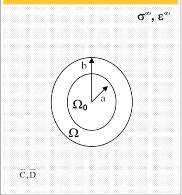
Based on elasticity theory and the Eshelby equivalent medium theory, [27] developed a three phase sphere model to estimate the effective shear modulus of two phase particulates composite. The three phase sphere model has as hypothesis a sphere of com-posite material embedded in the ininite medium of unknown effec-tive properties. To determine the elastic properties for this model, the sphere is composed initially by two phases, the matrix (domain Ω) and the inclusion (domain
Ω
0), the radii of these two spheres are b and a respectively (Figure 1). The volume fraction of the inclusion is taken as a relation between the radii and is given by3
=
b
a
f
IOn symmetric spherical loading condition, the strain in representa-tive element volume is spherically symmetrical [28], then the bulk modulus is expressed by Equation (28):
(28)
(
)(
)
(
)(
)
(
M M I I M)
M M M M I I
M
K
K
G
f
K
K
G
K
K
K
f
K
K
-+
+
+
-+
=
1
3
4
3
4
3
1
where KM and GM are the bulk modulus and shear modulus for the matrix, while KI and GI are the respective modulus for the inclusion and
K
is the bulk modulus of the composite.The three-phase model considers the sphere embedded in an in-inite and homogeneous medium (Figure 1), submitted to uniform stress and strain applied very distant from the inclusion. These stress and strain are named as
σ
∞ andε
∞, respectively. The bulk modulus K for this model is the same obtained for three-phase model (Equation 28), for two three-phases. Hypothetically, it is assumed that the displacement and traction acting on the contour of the body are uniform and linear.In the case of forced displacement, on the heterogeneous medium boundary, ESHELBY (1956) showed that the strain energy U, un -der applied displacement conditions, can be determined by Equa-tion (29) [12]:
(29)
(
)
ò
-=
i S i i ii
u
u
dS
U
U
0 00
2
1
s
s
where Si is the surface of the inclusion, U0 is the strain energy
in the same medium when it contains no inclusion,
σ
i0 andu
i0are the tractions and displacements in the same medium when it contains no inclusion and
σ
i andu
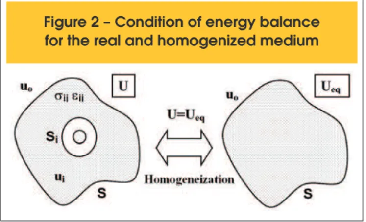
i are the corresponding quantities at the same point in the medium when it does contain the inclusion.Regarding the composite homogenization process, there is a re-lationship between the energies of the heterogeneous and homo-geneous medium, as presented in Equation (30) and observed in Figure 2:
(30)
0
0
U
U
U
U
U
U
=
eq\
eq=
\
=
Rewriting the Equation (29):
(31)
(
)
ò
-
=
i
S
i i i
i
u
u
dS
0
2
1
s
0s
0Applying the stress and strain in the radial and angular directions in Equation (31), results:
(32)
(
)
ò
+
+
-
-
-
=
i S e r e r r re e r e r re
r
u
u
u
u
u
u
dS
0
2
1
0 0 0 0 0 0f f q q f f q
q
t
s
t
t
t
s
The conditions of shear at the ininite for this problem are given by Equations (33) and (34):
(33)
ï
ï
ï
ï
þ
ïï
ï
ï
ý
ü
-=
=
=
-=
=
=
f
q
f
q
q
f
q
f
q
t
f
q
q
t
f
q
s
f q f q2
sin
2
cos
cos
2
cos
2
2
2
cos
cos
2
2
cos
2
1 0 1 0 2 1 0 1 0 1 0 2 1 0rsen
D
u
rsen
D
u
rsen
D
u
sen
sen
GD
sen
GD
sen
GD
r r r r(34)
( )
( )
( )
( )
( )
( )
ï
ï
ï
ï
þ
ïï
ï
ï
ý
ü
ú
û
ù
ê
ë
é
-+
+
-=
ú
û
ù
ê
ë
é
-+
+
+
=
ïþ
ï
ý
ü
ïî
ï
í
ì
ú
û
ù
ê
ë
é
-+
-=
34 53 1 34 53 1 34 53 1 31 22
1
1
4
16
2
2
2
1
1
4
8
2
cos
2
2
1
4
5
2
12
3
2
cos
2
r
D
r
D
D
sen
Gsen
r
D
r
D
D
Gsen
r
D
r
D
D
G
r
D
sen
e r e r ren
n
f
q
t
n
n
f
q
t
n
n
l
f
q
s
f qEvaluating Equation (32) for the effective shear modulus
G
, results:(35)
0
2=
+
÷÷
ø
ö
çç
è
æ
+
÷÷
ø
ö
çç
è
æ
C
G
G
B
G
G
A
M Mwhere A, B e C are listed in [11].
4.3 Hashin-Shtrikman Bounds
According to [29], Hashin-Shtrikman developed formulas for the upper and the lower bounds more accurate for the elastic modu-lus of homogeneous isotropic materials with arbitrary phase ge-ometry by deining a formulation based on the principles of linear elasticity theory.
Conclusions about the Hashin-Shtrikman bounds are: [14]
n If the composite material behave as a continuous two-phase composite, it satisies the boundaries;
n A truly two phase material must satisfy the bounds. If it does not, it can’t be considered as a two phase material;
n The proposition that, if the points are outside of the bounds, the material would not be two phase, implies that it could be assumed as having three or more phases in their constitution. The lower and upper bounds of Hashin-Shtrikman can be calcu-lated according to Equations (36) and (37), respectively [14, 30]:
(36)
(
)
(
)
ï
ï
ï
î
ï
ï
ï
í
ì
+
+
+
-+
=
+
+
-+
=
M M M M M M M i i M M M M M i i MG
K
G
G
K
f
G
G
f
G
G
G
K
f
K
K
f
K
K
4
3
5
2
6
1
4
3
3
1
inf inf(37)
(
)
(
)
ï
ï
ï
î
ï
ï
ï
í
ì
+
+
+
-+
=
+
+
-+
=
i i i i i i i M M i i i i i M M iG
K
G
G
K
f
G
G
f
G
G
G
K
f
K
K
f
K
K
4
3
5
2
6
1
4
3
3
1
sup supwhere Ki and Gi are the bulk and shear modulus of the inclusion, KM and GM are the bulk and shear modulus of the matrix and fi and fM are the respective volume fractions of these phases.
5. Methods
5.1 Experimental Evaluation
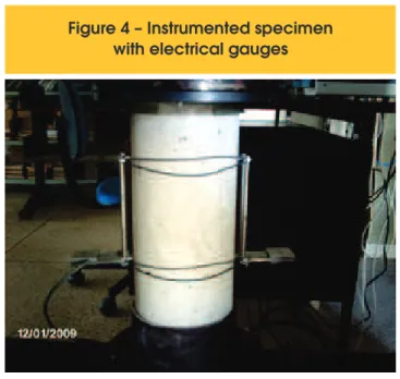
According to NBR 8522:2008 [4], the determining process of the concrete tangent elastic modulus must follow a script for the appli-cation of loading and also respect the characteristics of measuring devices and measurement bases. The loading process according to this standard, shown in Figure 3, is performed by cycles of load-ing and unloadload-ing searchload-ing compatibility of deformations. The methodology of the test according to NBR 8522:2008 was ix-ing stress, which evaluates the elastic modulus for a stress about 30% of the specimen rupture stress, previously tested. It is allowed that the upper limit of stress is changed based on any speciication. The dispositive used for measuring deformations in the specimens was electric gauges, with a load machine with capacity of 300 tons. The measuring the applied force was carried out by a loading cell with 30 tons capacity. Details of the execution of this test, with the instrumented specimen can be seen in Figure 4. The tests were performed in compression rigid plates (the upper one was articu-lated) with diameter 150 mm.
For the testing of the elastic modulus a number of three cylin-der specimens of 10 cm of diameter and 20 cm of height, for testing at ages 3 to 28 days, were molded. The proportions and other information about mixture are presented in Tables 4 and 5.
Mortar was extracted from each concrete type, coarse aggregate was eliminated by a screening process, and a number of two cy-lindrical specimens of 5 cm of diameter and 10 cm of height were
molded. Both concrete and mortar specimens were capped with cement and sulfur in a ratio 1:3, respectively.
The measurement of the strains was carried out by electrical
gag-Figure 3 – Loading cycles for determining the
concrete elastic modulus (NBR 8522:2008)
Figure 4 – Instrumented specimen
with electrical gauges
Table 4 – Characteristics of aggregates
Properties
Density (kg/m³)
diameter (mm)
Maximum
Fine modulus
Fine Aggregate
2560
2.40
2.24
Coarse Aggregate B0
2500
12.50
6.71
Coarse Aggregate B1
2500
19.00
7.96
Table 5 – Mixture proportions of the concrete
Mixture
(Cement:Sand:B0:B1:Water)
Proportions in mass
Volume fraction of
Cement Paste (f )
pc
T1
1 : 1.59 : 2.66 : 0 : 0.52
0.326
T2
1 : 1.59 : 0.8 : 1.86 : 0.52
0.326
T3
1 : 1.59 : 2.66 : 0 : 0.52
0.326
T4
1 : 0.99 : 0.6 : 1.4 : 0.39
0.368
T5
1 : 0.99 : 2 : 0 : 0.39
0.368
T6
1 : 0.99 : 2 : 0 : 0.39
0.368
T7
1 : 0.28 : 1.29 : 0 : 0.28
0.487
es using measurement basis of 100 mm and 50 mm, for concrete and mortar, respectively, as shown in Figure 4.
The results of the determinations of the elastic modulus of the con-crete for average values are presented in Table 6.
5.2 Numerical simpliications.
The following simpliications were adopted in the modeling: n The constituent phases and the effective composite material
are assumed to be isotropic, within the linear elastic region. n The aggregate is considered inert and maintains its elastic
properties over time.
n The aggregate is assumed with spherical shape.
n It is assumed that the transition zone between the coarse ag-gregate and the mortar has constant volume fraction.
n The elastic modulus of the ITZ is assumed to be constant throughout its thickness
The determination of ITZ elastic modulus employed a numerical formulation based on the inversion of the Equation (28) and Equa-tion (35) and the use of experimental results.
The analysis of concrete elastic modulus considering the interfa-cial transition zone (ITZ) is performed as follows:
n Effective Matrix (Mortar + ITZ) + Aggregate = Concrete. The elastic modulus of mortar + ITZ is obtained by a series model. The series model is described in [3] as: (Equation 38)
(38)
2 2 1 1
1
E
f
E
f
E
=
+
6. Concrete Microscopy
For the concrete used in this research a SEM-analysis was ac -complished in order to assess the thickness of the ITZ as well as its evolution over time, these results were compared to the informa-tion found in the literature.
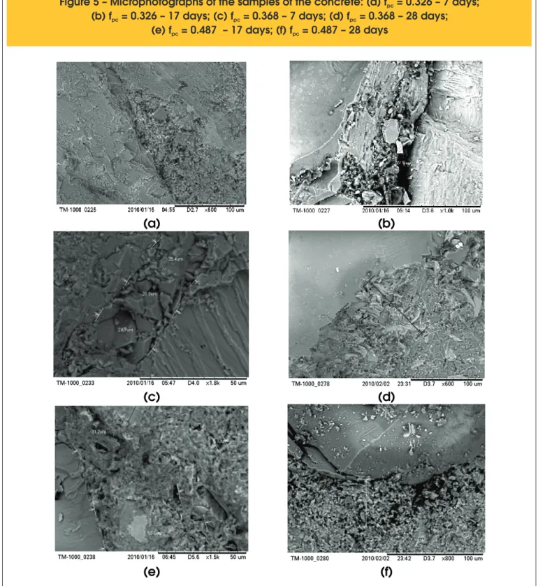
The tests were performed at the age of 28 days and less in order to verify, through identiication of ITZ, if there was variation over time of its thickness. In [31] was observed that the higher porosity that characterizes the transition zone occurs within a minimum of 30 µm. In Figure 5 are presented microphotographs of samples of concrete studied at the age of 28 days. The variable fpc represents the volume fraction of cement paste of the concrete produced. As a result of the evaluation of these images, it was observed that the thickness of ITZ is not much different between the two types of concrete, ranging from 30 µm to 100 µm, conirming the informa-tion presented by the technical literature.
7. Results and Discussion
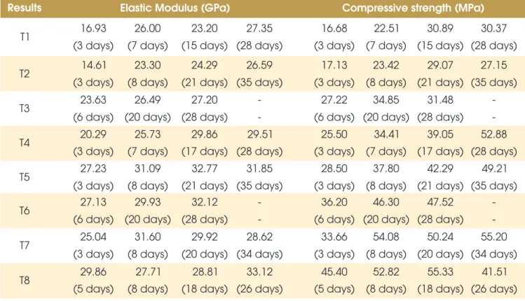
Elastic properties of the coarse aggregate are given in Table 6. In Tables 7 and 8 are shown the average values of elastic modulus and compressive strength obtained from the lab test described in the NBR 8522:2008 for concrete and mortar, respectively.
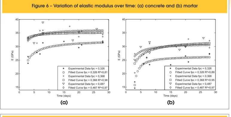
Poisson’s ratio for mortar was assumed as 0.17 and the elastic modulus of mortar and concrete are shown in Figure 6.
Experimental data were obtained using NBR 8522:2008 and the curves were itted using polynomial models based on the average values (3 samples each one) for the selected ages. Conidence intervals for small samples were veriied by the method of Student t with 95% of signiicance.
The change on time of concrete elastic modulus according to na-tional codes (listed in section 3), for three selected volume frac-tions of cement paste, are shown in Figure 7.
From the analysis of code expressions and experimental data it may be noted that:
n The mathematical expression of NBR 6118:2003, for ages of 15 days or more, results in errors up to 8% compared to the experimental data;
n Using the CEB/90 expression it was found better it, with errors lower than those calculated by NBR 6118:2003 expression; n The results calculated by ACI/95 and NBR 6118:2003
expres-sions are similar.
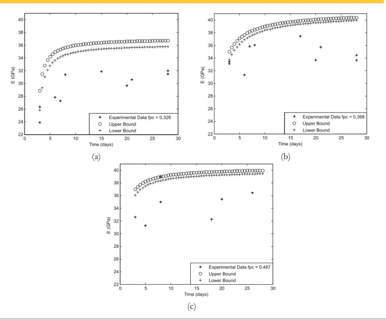
n High errors were obtained by using EUROCODE2/92 expression. Figure 8 presents the comparative analysis of experimental data by curves generated for the Hashin-Strikman bounds for concrete re-garding cement paste volume fractions of 0.326, 0.368 and 0.487. The Hashin-Shtrikman bounds are used to characterize two-phase composite and, if these limits are exceeded, denotes the presence of one or more extra phases.
It is observed from Figure 8 that almost all experimental points lie outside the bounds proposed by Hashin-Strikman, which implies that the concrete material must be evaluated considering the ITZ as a phase.
The variation over time of the elastic modulus of the Mori-Tanaka and three-phase sphere models in the range of 3 days to 28 days are shown in Figure 9.
The input data to analyze the application of three-phase sphere model are the elastic modulus, Poisson’s ratio and volume frac-tion of phases. The mortar elastic modulus was considered vary-ing over time (Figure 6) and Poisson’s ratio of mortar was con-sidered constant.
It is observed that the application of micromechanical models with-out the transition zone is not satisfactory, showing high errors com-pared to the experimental itted curves.
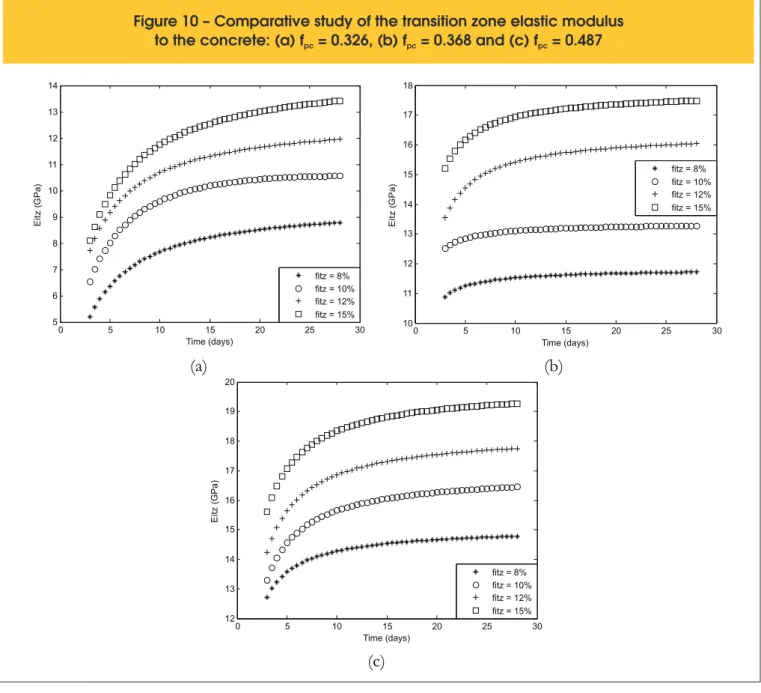
By applying the three phase sphere model, with the inversion of the equations as outlined in the methodology, is determined the ITZ elastic modulus (Figure 9). These curves were obtained by inversion of equations of three phase sphere model, considering the variation of volume fraction of the transition zone in relation to the total mixture.
The curves presented in Figure 10 shows the direct inluence of the volume fraction of ITZ and, consequently, its thickness, on the concrete elastic modulus. These values were obtained from the experimental data and show an evolution over time similar to the concrete and mortar.
Table 6 – Elastic modulus and Poisson's
ratio of coarse aggregate
Elastic Modulus
57 GPa
Making use of the results shown in Figure 10, the concrete elas-tic modulus has been calculated by direct application of the three phase sphere model according to Equation (38) and it is presented in Figures 11 and 12.
The relationships proposed in the literature refer to the transition zone elastic modulus ranging around 30% to 50% of the matrix elastic modulus, in general, compared to the cement paste matrix. In the analysis considering the matrix made of mortar, which
in-Figure 5 – Microphotographs of the samples of the concrete: (a) f = 0.326 – 7 days;
pc(b) f = 0.326 – 17 days; (c) f = 0.368 – 7 days; (d) f = 0.368 – 28 days;
pc pc pc(e) f = 0.487 – 17 days; (f) f = 0.487 – 28 days
pc pc(a)
(b)
(c)
(d)
Table 7 – Average values of elastic modulus and compressive strength of the concrete
Results
Elastic Modulus (GPa)
Compressive strength (MPa)
T1
23.84
27.25
31.87
31.95
13.37
20.40
25.33
27.56
(3 days) (7 days)
(15 days)
(28 days)
(3 days)
(7 days)
(15 days)
(28 days)
T2
26.31
31.35
30.58
31.91
13.79
19.25
23.89
25.89
(3 days)
(8 days)
(21 days)
(35 days)
(3 days)
(8 days)
(21 days)
(35 days)
T3
27.82
29.63
31.48
-
22.90
26.14
30.11
-
(6 days) (20 days)
(28 days)
-
(6 days)
(20 days)
(28 days)
-
T4
33.09
35.83
37.44
34.40
22.26
32.04
33.38
38.12
(3 days) (7 days)
(17 days)
(28 days)
(3 days)
(7 days)
(17 days)
(28 days)
T5
33.39
36.04
35.70
35.22
24.65
33.46
37.46
41.16
(3 days) (8 days)
(21 days)
(35 days)
(3 days)
(8 days)
(21 days)
(35 days)
T6
31.33
32.21
32.70
-
30.02
32.21
42.40
-
(6 days)
(20 days)
(28 days)
-
(6 days)
(20 days)
(28 days)
-
T7
32.56
38.93
35.41
37.13
34.89
40.98
46.07
47.30
(3 days) (8 days)
(20 days)
(34 days)
(3 days)
(8 days)
(20 days)
(34 days)
T8
31.26
34.99
32.25
36.43
39.07
45.45
47.62
45.96
(5 days) (8 days)
(18 days)
(26 days)
(5 days)
(8 days)
(18 days)
(26 days)
Table 8 – Average values of elastic modulus and compressive strength of the mortar
Results
Elastic Modulus (GPa)
Compressive strength (MPa)
T1
16.93
26.00
23.20
27.35
16.68
22.51
30.89
30.37
(3 days)
(7 days)
(15 days)
(28 days)
(3 days)
(7 days)
(15 days)
(28 days)
T2
14.61
23.30
24.29
26.59
17.13
23.42
29.07
27.15
(3 days)
(8 days)
(21 days)
(35 days)
(3 days)
(8 days)
(21 days)
(35 days)
T3
23.63
26.49
27.20
-
27.22
34.85
31.48
-
(6 days)
(20 days)
(28 days)
-
(6 days)
(20 days)
(28 days)
-
T4
20.29
25.73
29.86
29.51
25.50
34.41
39.05
52.88
(3 days)
(7 days)
(17 days)
(28 days)
(3 days)
(7 days)
(17 days)
(28 days)
T5
27.23
31.09
32.77
31.85
28.50
37.80
42.29
49.21
(3 days)
(8 days)
(21 days)
(35 days)
(3 days)
(8 days)
(21 days)
(35 days)
T6
27.13
29.93
32.12
-
36.20
46.30
47.52
-
(6 days)
(20 days)
(28 days)
-
(6 days)
(20 days)
(28 days)
-
T7
25.04
31.60
29.92
28.62
33.66
54.08
50.24
55.20
(3 days)
(8 days)
(20 days)
(34 days)
(3 days)
(8 days)
(20 days)
(34 days)
T8
29.86
27.71
28.81
33.12
45.40
52.82
55.33
41.51
(a)
(b)
0 5 10 15 20 25 30
15 20 25 30 35
E
(G
P
a)
Time (days)
Experimental Data fpc = 0,326 Fitted Curve fpc = 0,326 R²=0,81 Experimental Data fpc = 0,368 Fitted Curve fpc = 0,368 R²=0,98 Experimental Data fpc = 0,487 Fitted Curve fpc = 0,487 R²=0,97
0 5 10 15 20 25 30
15 20 25 30 35
Time (days)
E
(G
P
a)
Experimental Data fpc = 0,326 Fitted Curve fpc = 0,326 R²=0,89 Experimental Data fpc = 0,368 Fitted Curve fpc = 0,368 R²=0,95 Experimental Data fpc = 0,487 Fitted Curve fpc = 0,487 R²=0,97
Figure 7 – Comparative study of the evolution over time of the concrete elastic
modulus with code expressions: (a) f = 0.326, (b) f = 0.368 and (c) f = 0.487
pc pc pc(a)
(b)
(c)
0 5 10 15 20 25 30
20 25 30 35 40 45
Time (days)
E
(G
P
a)
Experimental Data fpc = 0,326 Fitted Curve fpc = 0,326 R²=0,81 NBR 6118:2003
CEB/90 ACI/95 NB1/80 EC2/92
0 5 10 15 20 25 30
20 25 30 35 40 45
Time (days)
E
(G
P
a)
Experimental Data fpc = 0,368 Fitted Curve fpc = 0,368 R²=0,98 NBR 6118:2003
CEB/90 ACI/95 NB1/80 EC2/92
0 5 10 15 20 25 30
20 25 30 35 40 45
E
(G
P
a)
Time (days)
Experimental Data fpc = 0,487 Fitted Curve fpc = 0,487 R²=0,97 NBR 6118:2003
Figure 8 – Hashin-Shtrikman bounds for concrete: (a) f = 0.326, (b) f = 0.368 and (c) f = 0.487
pc pc pc(a)
(b)
(c)
0 5 10 15 20 25 30
22 24 26 28 30 32 34 36 38 40
Time (days)
E
(G
P
a)
Experimental Data fpc = 0,326 Upper Bound
Lower Bound
0 5 10 15 20 25 30
22 24 26 28 30 32 34 36 38 40
Time (days)
E
(G
P
a)
Experimental Data fpc = 0,368 Upper Bound
Lower Bound
0 5 10 15 20 25 30
22 24 26 28 30 32 34 36 38 40
Time (days)
E
(G
Pa
)
Experimental Data fpc = 0,487 Upper Bound
Lower Bound cludes the cement paste and ine aggregate particles, this relation
-ship is in a larger interval than that presented in the references. Ad-ditionally, the relationship varies over time because, as the mortar, the transition zone has its strength and rigidity increased over time.
8. Conclusions
The following conclusions may be written:
n The expression proposed by NBR 6118:2003 presents accept-able dispersions in relation to the experimental data obtained, but knowing the relationship with the phase’s properties, it could be predicted an adjusting coeficients to better charac-terize the local concrete in Brazil.
n The CEB/90 expression was the best itting to the experimental curves, and there were observed similar results for the applica-tion in [17] and [22].
n The behavior of the elastic modulus shows a strong de-pendence on the cement paste volume fraction, which was expected because cement paste has a great inluence on the concrete quality. Time in another important parameter because both compressive strength and elastic modulus de-pends on it.
n The proposition of the elastic modulus as a function of some dosage parameters is important to evaluate the in-fluences of the phases in determining the concrete elastic modulus.
Figure 9 – Comparative study of the application of micromechanical models without transition zone:
(a) f = 0.326, (b) f = 0.368 and (c) f = 0.487
pc pc pc(a)
(b)
(c)
0 5 10 15 20 25 30
22 24 26 28 30 32 34 36 38
Time (days)
E
(G
P
a)
Experimental Data fpc = 0,326 Fitted Curve fpc = 0,326 R²=0.81 Three Phase Sphere Model Mori-Tanaka Model
0 5 10 15 20 25 30
31 32 33 34 35 36 37 38 39 40 41
E
(G
P
a)
Time (days)
Experimental Data fpc = 0,368 Fitted Curve fpc = 0,368 R²=0.98 Three Phase Sphere Model Mori-Tanaka Model
0 5 10 15 20 25 30
31 32 33 34 35 36 37 38 39 40 41
Time (days)
E
(G
Pa
)
Experimental Data fpc = 0,487 Fitted Curve fpc = 0,487 R²=0.97 Three Phase Sphere Model Mori-Tanaka Model
results the transition zone volume fraction is between 10% and 12% and has variable thickness.
n Data reported in the literature show that the ratio of elastic modulus of the transition zone and cement paste varies be-tween 0.3 and 0.5 and, according to the results, this ratio is the same for the mortar and its transition zone.
n The use of transition zone with the matrix of mortar through a series model, when associated to the micromechanical model, showed good results.
n It is possible to conclude on the necessity of consideration of the tran-sition zone for determining the elastic properties of the concrete.
9. Acknowledgments
The authors thank CNPq for the inancial support.
10. References
[01] HAECKER, C.-J., GARBOCZI, E. J., BULLARD, J. W., BOHN, R. B., SUN, Z., SHAH, S. P., VOIGT, T. Modeling the linear elastic properties of Portland cement paste. Cement and Concrete Research, v.35, 2005; p.1948-1960.
[02] REVISTA CONCRETO E CONSTRUÇÕES, Módulo de elasticidade é parâmetro fundamental para a durabilidade da estrutura de concreto, IBRACON, n.48, 2007.
Figure 10 – Comparative study of the transition zone elastic modulus
to the concrete: (a) f = 0.326, (b) f = 0.368 and (c) f = 0.487
pc pc pc(a)
(b)
(c)
0 5 10 15 20 25 30
5 6 7 8 9 10 11 12 13 14
Time (days)
E
itz
(G
Pa
)
fitz = 8% fitz = 10% fitz = 12% fitz = 15%
0 5 10 15 20 25 30
10 11 12 13 14 15 16 17 18
Time (days)
E
itz
(G
P
a)
fitz = 8% fitz = 10% fitz = 12% fitz = 15%
0 5 10 15 20 25 30
12 13 14 15 16 17 18 19 20
Time (days)
E
itz
(G
Pa
)
fitz = 8% fitz = 10% fitz = 12% fitz = 15%
TÉCNICAS. Concreto – Determinação do módulo estático de elasticidade à compressão. NBR 8522, Rio de Janeiro, 2008.
[05] BESHR, H., ALMUSALLAM A. A., MASLEHUDDIN, M. Effect of coarse aggregate quality on the mechanical properties of high strength concrete. Construction and Building Materials, v.17, 2003; p.97-103,
[06] WU, K.-R., LIU, J.-L., ZHANG, D., YAN, A. Rupture probability of coarse aggregate on fracture surface of concrete. Cement and Concrete Research, v.29, 1999; p.1983-1987.
[07] ZHAO, X.-H., CHEN, W. F. Effective elastic moduli of concrete with interface layer. Computers and Structures, v.66, n.2-3, 1998; p.275-288.
[08] NADEAU, J. C. A multiscale model for effective moduli of concrete incorporating ITZ, water-cement ratio gradients, aggregate size distributions, and entrapped voids. Cement and Concrete Research, v.33, 2003; p.103-113.
[09] WU, K.-R., CHEN, B., YAO, W., ZHANG, D. Effect of coarse aggregate type on mechanical properties of high-performance concrete. Cement and Concrete Research, v.29, 2001; p.1983-1987.
[10] MEHTA, P. K., MONTEIRO, P. J. M. Concreto: estrutura, propriedades e materiais. Ed. PINI, 1ª ed., São Paulo, 1994.
Figure 11 – Comparative study of the concrete elastic modulus obtained with
three phase sphere model: (a) f = 0.326, (b) f = 0.368 and (c) f = 0.487
pc pc pc(a)
(b)
(c)
0 5 10 15 20 25 30
20 22 24 26 28 30 32
Time (days)
E
(G
Pa
)
Experimental Data fpc = 0,326 Fitted Curve fpc = 0,326 R²=0.81 ETF fitz=8%
ETF fitz=10% ETF fitz=12% ETF fitz=15%
0 5 10 15 20 25 30
30 31 32 33 34 35 36 37 38
Time (days)
E
(G
P
a)
Experimental Data fpc = 0,368 Fitted Curve fpc = 0,368 R²=0.98 ETF fitz=8%
ETF fitz=10% ETF fitz=12% ETF fitz=15%
0 5 10 15 20 25 30
31 32 33 34 35 36 37 38 39
Time (days)
E
(G
P
a)
Experimental Data fpc = 0,487 Fitted Curve fpc = 0,487 R²=0.97 ETF fitz=8%
ETF fitz=10% ETF fitz=12% ETF fitz=15% Solids, v.27, 1979; p.315-330.
[12] LI, G., ZHAO, Y., PANG, S.-S. Four-phase sphere modeling of effective bulk modulus of concrete. Cement and Concrete Research, v.29, 1999; p.839-845.
[13] MONTEIRO, P. J. M. Caracterização da microestrutura do concreto: fases e interfaces; aspectos de durabilidade e de microissuração. São Paulo, 1993, Tese (Livre Docência) - Escola Politécnica, Universidade de São Paulo, 138 p. [14] LI, G., ZHAO, Y., PANG, S.-S., LI, Y. Effective Young’s
modulus estimation of concrete. Cement and Concrete Research, v.29, 1999; p.1455-1462. [15] NEVILLE, A. M. Propriedades do concreto. Ed. PINI,
2ª ed., São Paulo, 1997.
[16] ARAÚJO, J. M. O módulo de deformação longitudinal do concreto. Revista Teoria e Prática na Engenharia Civil, n.1, 2000; p.9-16.
[17] MELO NETO, A. A., HELENE, P. R. L. Módulo de elasticidade: dosagem e avaliação de modelos de previsão do módulo de elasticidade de concretos.
In: Congresso Brasileiro do Concreto, 44º, Belo Horizonte, 2002, Anais.
[18] MEIRELES NETO, M., ALBUQUERQUE, A. T., CABRAL, A. E. B. Estudo do módulo de elasticidade de concretos produzidos em Fortaleza – CE – Brasil.
In: XXXIV Jornadas Sudamericanas de Ingenería
Estructural, San Juan – Argentina, 2010, Anais. [19] PERSSON, B. Justiication of fédération international
Figure 12 – Comparative study of the concrete elastic modulus obtained
with Mori-Tanaka model: (a) f = 0.326, (b) f = 0.368 and (c) f = 0.487
pc pc pc(a)
(b)
(c)
0 5 10 15 20 25 30
20 22 24 26 28 30 32
Time (days)
E
(G
P
a)
Experimental Data fpc = 0,326 Fitted Curve fpc = 0,326 R²=0.81 MT fitz=8%
MT fitz=10% MT fitz=12% MT fitz=15%
0 5 10 15 20 25 30
30 31 32 33 34 35 36 37 38
Time (days)
E
(G
P
a)
Experimental Data fpc = 0,368 Fitted Curve fpc = 0,368 R²=0.98 MT fitz=8%
MT fitz=10% MT fitz=12% MT fitz=15%
0 5 10 15 20 25 30
31 32 33 34 35 36 37 38 39
E
(G
P
a)
Time (days)
Experimental Data fpc = 0,487 Fitted Curve fpc = 0,487 R²=0.97 MT fitz=8%
MT fitz=10% MT fitz=12% MT fitz=15%
normal and high-performance concrete, HPC. Cement and Concrete Research, v.34, 2004; p.651-655.
[20] SANTOS, S. B., GAMBALE, E. A., ANDRADE, M. A. S. Modelos de predição do módulo de elasticidade do concreto. In: Congresso Brasileiro do Concreto, 48º, Rio de Janeiro, 2006, Anais. [21] ARAÚJO, J. M. Modelos para previsão do módulo
de deformação longitudinal do concreto: NBR 6118 versus CEB. Revista Teoria e Prática na Engenharia Civil, n.12, 2008; p.81-91.
[22] DA GUARDA, M. C. C. Cálculo de deslocamentos em pavimentos de edifícios de concreto armado. São Paulo, 2005, Tese (Doutorado), Escola de Engenharia de São Carlos – USP.
[23] BENVENISTE, Y. A new approach to the application of Mori –Tanaka’s theory in composite material. Mechanics of Materials, v.6, 1987; p.147-157. [24] YANG, C- C., HUANG, R. Double inclusion model for
approximate elastic moduli of concrete material. Cement and Concrete Research, v.26, n.1, 1996; p.83-91.
[25] YANG, C- C., HUANG, R. A two-phase model for predicting the compressive strength of concrete. Cement and Concrete Research, v.26, n.10, 1996; p.1567-1577.
[26] QU, J., CHERKAOUI, M. Fundamentals of
micromechanics of solids, John Wiley & Sons, 2006. [27] CHRISTENSEN, R. M.; LO, K. H. (1979). Solutions
and cylinder models, Journal Mechanics and Physics Solids, Vol. 27, p. 315-330.
[28] NEMAT-NASSER, S., HORI, M. Micromechanics: overall properties of heterogeneous materials. Second Revised Edition, Elsevier, North-Holland, 1999.
[29] HERNÁNDEZ, M. G., ANAYA, J. J., ULLATE, L. G., IBAÑEZ, A. Formulation of a new micromechanic model of three phases for ultrasonic characterization of cement-based materials. Cement and Concrete Research, v.36, 2006; p.609-616.
[30] SIMEONOV, P., AHMAD, S. Effect of transition zone on the elastic behavior of cement-based composites. Cement and Concrete Research, v.25, n.1, 1995; p.165-176.