A STUDY OF in situ DEGRADABILITY: HETEROGENEITY OF VARIANCES AND CORRELATED ERRORS

(1)

A STUDY OF

in situ

DEGRADABILITY: HETEROGENEITY

OF VARIANCES AND CORRELATED ERRORS

Taciana Villela Savian1_{; Joel Augusto Muniz}2_*

1

UFLA - Programa de Pós-Graduação em Agronomia/Estatística e Experimentação Agropecuária.

2

UFLA - Depto. de Ciências Exatas, C.P. 3037 - 37200-000, Lavras, MG - Brasil. *Corresponding author <joamuniz@ufla.br>

ABSTRACT: Degradation models exhibit a non-linear behavior and the selection of a model to describe the degradability depends on the coherence of the model with the involved biological events. The purpose of this study is to evaluate the behavior of the parameters of the degradation model proposed by Mertens & Loften, adjusted to the results of an in situ degradability trial. The experiment evaluated the potential degradable residue of neutral detergent fiber (NDF) of coastcross grass (Cynodon

dactylon × Cynodon nlemfuensis) submitted to two cutting ages (30 and 90 days), with three replicates.

For each cutting age, the potentially degradable residue of NDF was studied using fifteen incubation times (0; 0,5; 1; 3; 6; 9; 12; 18; 34; 35; 48; 56; 72; 96 e 120 hours). The experimental unit comprised one non-lactating cow with a permanent ruminal fistula. Mean and individual adjustments were obtained for the animals in three different configurations: inverse variance weight without autoregressive errors; unweighted with autoregressive errors, and unweighted without autoregressive errors. Variances of parameter estimators were also obtained by means of the mean parameter covariance matrix, providing expressions for the estimation of the confidence age for the parameters of the model. A weighting of the model by the inverse variance resulted in estimates statistically equal to zero for the colonization time. The use of a structure of second order autoregressive errors improved the fit of the model of Mertens & Loften, providing more precise estimates of the parameters.

Key words: ruminal degradability, non-linear regression, parameters estimation, coast-cross grass

UM MODELO DE DEGRADABILIDADE

in situ

: HETEROGENEIDADE

DE VARIÂNCIAS E ERROS CORRELACIONADOS

RESUMO: Os modelos de degradação mostram um comportamento não-linear e a seleção de um modelo para descrever a degradabilidade depende da coerência deste com os eventos biológicos. Objetivou-se avaliar o comportamento dos parâmetros do modelo de degradação proposto por Mertens & Loften ajustado aos resultados de um ensaio de degradabilidade in situ. O experimento avaliou o resíduo potencialmente degradável da fibra em detergente neutro (FDN) da gramínea coast-cross

(Cynodon dactylon × Cynodon nlemfuensis) submetida a duas idades de corte (30 e 90 dias), com três

repetições. Em cada idade de corte, o resíduo potencialmente degradável da FDN foi estudado utilizando quinze tempos de incubação (0; 0,5; 1; 3; 6; 9; 12; 18; 34; 35; 48; 56; 72; 96 e 120 horas). A unidade experimental foi constituída por uma vaca não lactante, com fístula ruminal permanente. Foram obtidos ajustes médios e individuais para os animais, em três diferentes configurações: ponderado pelo inverso da variância sem erros auto-regressivos; não ponderado com erros auto-regressivos (AR) e não ponderado sem erros auto-regressivos. Obtiveram-se também as variâncias dos estimadores dos parâmetros por meio da matriz de covariâncias dos parâmetros, propondo-se expressões para a estimação do intervalo de confiança para os parâmetros do modelo. A ponderação do modelo, pelo inverso da variância, proporcionou estimativas estatisticamente iguais a zero para o tempo de colonização das partículas. A consideração de uma estrutura de erros auto-regressivos de segunda ordem melhorou o ajuste do modelo, promovendo estimativas mais precisas para os parâmetros.

Palavras-chave: degradabilidade ruminal, regressão não-linear, estimação de parâmetros, gramínea coast-cross

INTRODUCTION

Waldo, in 1970, was the first to show that degradation profiles were combinations of digestible and indigestible materials and that the potentially

(2)

inclusion of a parameter for the parameter estimates of the first order model of Waldo et al. (1972) which examines this period, for the degradability in situ and

in vitro of the NDF.

Several important statistical considerations, normally not taken into account in the study of rumi-nal degradation curves, are the heterogeneity the vari-ance and the existence of autocorrelation between the adjustment residues. If such aspects are ignored in the adjustment process, respective to these facts, biased estimates and an underestimation of the variances of the parameters may result (Souza, 1998). In accor-dance with Hoffman & Viera (1998), in the presence of the heterogeneity of variance, the use of the weighted least squares method is more adequate for forming estimates that are unbiased and of minimum variance; in addition, in the presence of variance het-erogeneity and autocorrelation of the residues, the gen-eralized least squares method is more efficient than the weighted and ordinary least squares method.

In the case of the study of nonlinear models that describe ruminal degradation, it is reasonable to incorporate autocorrelation, seeing that the means of degradation of the actual nutritional component of in-terest are taken from one animal, and, therefore, prob-ably correlated.

This research evaluates the behavior of the pa-rameter estimate for the ruminal degradability model proposed by Mertens & Loften (1980) and obtains ex-pressions for the variance of its parameter estimators, which takes into consideration an autoregressive er-ror structure weighted for the inverse of variance, in this manner, tests for the actual existence of biologi-cally interpretable parameters in the model.

MATERIAL AND METHODS

To illustrate the methodology, this study makes use of experimental data (Reis, 2000) related to the potentially degradable residue of neutral detergent fi-ber (NDF) of coastcross grain (Cynodon dactylon ×

Cynodon nlemfuensis) subjected to two different cut-ting ages (30 and 90 days). For each cutcut-ting age, the degradation profile was evaluated for fifteen incuba-tion times (0; 0.5; 1; 3; 6; 9; 12; 18; 24; 36; 48; 56; 72; 96 and 120 hours), the experimental unit consist-ing of a non-lactant cow with a permanent ruminant fistula.

The model used to describe the potentially de-gradable residue was that of Mertens & Loften (1980), as shown by:

( )

⎩ ⎨ ⎧

> +

< < +

= − − ,

0

L t to I De

L t to I D t

R ct L

in which : R(t) is the residue after incubation in the ru-men at time t (%); D is the degradable fraction (%); c is the degradation rate (hours-1); t is the incubation time (hours); I is the insoluble and non-degradable fraction (%) and L is the colonization time or lag time (hours).

Parameter estimates for the individual curves and parameter estimates for the mean curve were ob-tained by means of: ordinary least squares (OLS), when the residual structure does not violate any of the presuppositions; weighted least squares (WLS), when the assumption of homogeneity of variances was vio-lated and generalized least squares (GLS) when the as-sumption of residual independence was violated. In the process of estimation of the parameters of the nonlin-ear model, the solution for the systems of nonlinnonlin-ear normal equations was obtained by the iterative Gauss-Newton method.

In the case of weighted nonlinear models, the “Weight” option of the proc model was employed, and, in order to verify the presence of residual autocorrelation, the macro %AR(y,p) was used, imple-mented in the same module (SAS, 1995), together with the analysis of correlograms. Only the animals that dis-played autocorrelation of the first or second order and when the weighting was necessary, were used in the adjustments.

The estimates of the asymptotic covariance matrix are presented by Draper & Smith (1998) in the following form: Vˆ ( ) ( ' )θ =ˆ X X QME, in which; X is the matrix of the partial derivatives of the model in re-lation to the parameters, and QME is the residual mean square. In this form the confidence age was defined by the parameter θ_j as:

) ˆ ( ˆ ˆ

)

( j j t(gl.error,₂) V j

ICθ =θ ± α θ

in which: θˆ_j is the estimate of the j-th parameter of the model; t(gl.error,α₂) is the highest percentile α2 of

the Student t-distribution for the degree of freedom of the residue and

( )

ˆ ˆ

j

V θ

is the estimate of the variance of the estimate of the j-th parameter.

RESULTS AND DISCUSSION

(3)

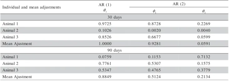
s t n e m t s u j d a n a e m d n a l a u d i v i d n

I AR(1)

φ₁

) 2 ( R A

φ₁ φ₁

s y a d 0 3

1 l a m i n

A 0.9725 0.8728 0.2269

2 l a m i n

A 0.1026 0.0020 0.0040

3 l a m i n

A 0.8526 0.6677 0.0599

t n e m t s u j A n a e

M 1.0000 0.9281 0.0591

s y a d 0 9

1 l a m i n

A 0.0759 0.1153 0.7132

2 l a m i n

A 0.7761 0.5307 0.1575

3 l a m i n

A 0.5347 0.4765 0.3779

t n e m t s u j A n a e

M 0.8849 0.5124 0.2134

Table 2 - The significance of the autocorrelation parameters for the individual and mean adjustments, for each cutting age, taking into account the first and second order autoregressive error structure.

Table 1 - Mean observed values of potentially degradable NDF residue, in percentage, for each cutting age over the elapse of incubation time and their respective variances, in squared percentage.

) r u o h ( e m i

T 30days Variance 90days Variance

0 70.99 476.1567 72.92 373.9185

5 .

0 70.96 476.7667 72.86 374.4880

1 70.93 476.4194 72.80 374.6088

3 70.85 477.2406 72.46 385.1181

6 66.31 401.8949 71.91 398.3022

9 64.64 382.2124 69.58 365.5008

2

1 63.44 351.7139 65.92 282.5570

8

1 58.30 322.7611 60.22 190.2345

4

2 52.56 199.1552 57.86 186.6237

6

3 49.40 193.8924 49.88 86.9305

8

4 46.20 188.0589 46.56 53.2182

6

5 45.25 199.4191 45.07 55.5179

2

7 44.64 217.8108 43.23 43.6195

6

9 42.74 236.6482 40.59 43.6382

0 2

1 40.89 206.6642 37.63 61.7197

7 7 3 5 .

2 9.1313

2 min 2 max/s

s

The relation between the greatest and the least variance was 2.54 for grass harvested at 30 days and does not display heterogeneity. For the grass cut at 90 days, the least variance is 9.13 times less than the greatest variance, a relationship that is significant for three experimental groups (three animals) and 14 de-grees of freedom, with a significance level of 5%, ac-cording to Hartley's maximum F-ratio (Pearson & Hartley, 1970).

Studying growth curves of bovines, Mazzini et al. (2005) and Silva et al. (2002), indicate that weighting by inverse variance is a viable solution for the occurrence of variance heterogeneity, yet it does

not solve the problem of residual autocorrelation, which requires the use of procedures with an autoregressive error structure. The ratio between the maximum and minimum variance was used by Mazzini (2001) to study growth curves of Hereford cattle. He indicates, to the extent that the age of the animals increased, there was an increment in the variances of the body weight, this being also another pattern of heteroscedascity.

(4)

When examining residual autocorrelation, Mazzini (2001), Mazzini et al. (2003; 2005) studied the growth curves of bovines by means of various func-tions and found that, in relation to the fitting of the mean curves, some functions did not fit an autoregressive model of first or second order; how-ever, when fitting individual curves, there were ani-mals that displayed these error structures.

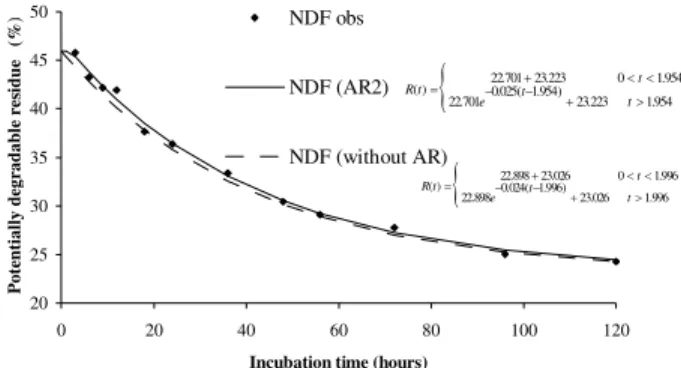
By means of a partial autocorrelation function for the Mertens & Loften (1980) model without weighting and without AR, it can be seen that the resi-dues follow an autoregressive error structure AR2 (Figure 1). For this same configuration, adjusting the same function and considering the error structure AR2, it may be seen, by the function of the autocorrelation, that the residues become independent (Figure 2).

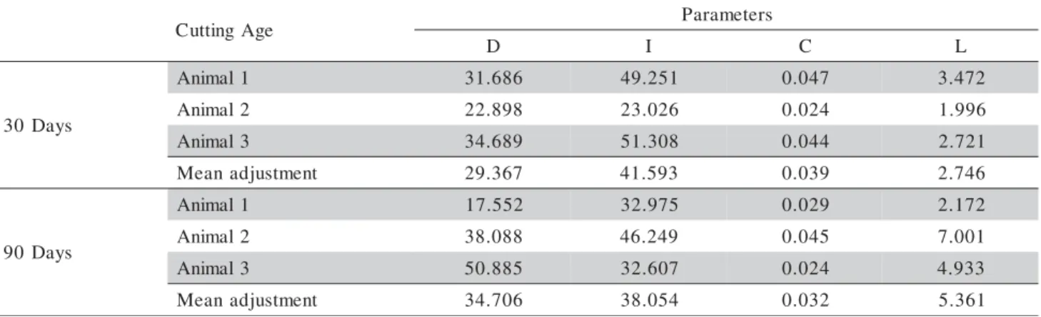
The parameters of the degradation model pro-posed by Mertens & Loften (1980) (Table 3) are esti-mated without taking into consideration the weight and structure of the correlated errors, for each animal as well as for the mean. For the adjustment of the mean curve, an increase was found in the value of the esti-mate of the colonization time (parameter L) for a grass cutting age of 90 days, probably because in plants of an advanced age there is a loss of water and a strong lignin complex with the components of the cellular wall. For the digestion process to occur, the microor-ganisms must penetrate the resistant barriers of the surface of the food particles to reach their preferred substrata, and the degree to which the microorganisms fix themselves and penetrate these physical barriers, reflects on the colonization time.

With regard to the values of the parameter es-timates, Feitosa (1999), in comparing models in tests of degradability in situ with coast-cross grass hay, ob-served that the model of McDonald (1981), also cor-rected for the colonization time, resulted in the same estimates as the model of Mertens & Loften (1980). McDonald (1981) gives values of 43.26% for the

in-soluble and nondegradable fraction; 4%.h-1 for the rate of degradation (parameter c) and 2.45 hours for the colonization time. This model was also used by Lira (2000) to predict the degradation of NDF of brachiaria grass (Brachiaria decumbens Stapf.) in two seasons (dry and rainy), showing mean values of 51.32% for the degradable fraction; 38.08% for the insoluble and nondegradable fraction; 2.5% h-1

for the rate of deg-radation and 7.64 hours for the colonization time in the rainy season.

According to the significant values for the autocorrelation estimates of the parameters (Table 2), the model was adjusted only for animal 2, for the grass cutting age of 30 days, with a second order

Table 3 - Estimate of the parameters for the unweighted model and without autoregressive error structure.

e g A g n i t t u

C Parameters

D I C L

s y a D 0 3

1 l a m i n

A 31.686 49.251 0.047 3.472

2 l a m i n

A 22.898 23.026 0.024 1.996

3 l a m i n

A 34.689 51.308 0.044 2.721

t n e m t s u j d a n a e

M 29.367 41.593 0.039 2.746

s y a D 0 9

1 l a m i n

A 17.552 32.975 0.029 2.172

2 l a m i n

A 38.088 46.249 0.045 7.001

3 l a m i n

A 50.885 32.607 0.024 4.933

t n e m t s u j d a n a e

M 34.706 38.054 0.032 5.361 Figure 1 - Partial autocorrelation function adjusted for the

unweighted model without AR, for animal no. 2, with a grass cutting age of thirty days.

(5)

autoregressive error structure AR(2). In Figure 3 it is possible to observe the data adjustment to the model of Mertens & Loften (1980), whether or not the sec-ond order autoregressive error structure was used.

Values of the estimates of the parameters, in considering the error structure AR(2), do not undergo large changes (Table 4). The estimates of the variance of the parameter estimate, obtained by the variance-covariance matrix for this same configuration, shows significant reduction in their values, resulting in con-fidence ages of less amplitude and more precise pa-rameter estimates. This methodology was also used by Pereira et al. (2005) for the prediction of mineralized nitrogen in latosols by means of nonlinear models. In comparing confidence ages obtained by means of a variance-covariance matrix of parameters, the author also established lower estimates of parameter variance. With the increase in incubation time of the samples in the rumen, there was a decrease in the re-sidual variances of NDF of the potential degradable resi-dues of the coastcross grass for the cutting age of 90 days (Table 1). The parameter estimates for the Mertens & Loften (1980) model are in Table 5, with and with-out weighting, with the respective variance estimates obtained for the parameter covariance matrix for each animal and their mean. The adjustment of Mertens & Loften (1980) model to the data, whether or not weight-ing is used, can be seen in Figures 4 and 7, for each one of the animals and their mean, respectively.

In the curve adjustment for animals 1 and 3 (Table 5), the values of parameter estimates referring to the non-degradable fraction (parameter I), rate of degradation (parameter c) and colonization time (pa-rameter L) undergo reductions when weighting is in-troduced into the model. For this last parameter, the reduction together with the increase of the variance estimate rise to nonsignificant, signifying that the po-tentially degradable residue of NDF of coastcross grass begins to undergo substantial losses as soon as

incu-s r e t e m a r a

P WithoutAR(2) WithAR(2)

I

L 1 _L_S1 _L_I1 _L_S1

D 22.898 0.478 21.375 24.421 22.701 0.075 22.099 23.304

I 23.026 0.395 21.643 24.409 23.223 0.045 22.757 23.688

C 0.024 3.0× 10-6 ₀_.₀₂₀ ₀_.₀₂₈ ₀_.₀₂₅ ₃_.₀_× ₁₀-7 ₀_.₀₂₃ ₀_.₀₂₆ L 1.996 0.663 0.204 3.788 1.954 0.125 1.177 2.731

-- --- --- --- -0.918 0.046 -1.389 -0.448

-- --- --- --- -0.853 0.053 -1.358 -0.347

Table 4 - Parameter estimate, estimate of the variance of the parameter estimate for the model, with and without AR(2) - (30 days - Animal 2), obtained by the covariance matrix of parameters and lower and upper limit of a 95% confidence age.

1- LI(lower limit), LS (upper limit)

φ

2

φ

) ˆ ( ˆ_θ

V

) ˆ ( ˆ_θ

V

θˆ _θˆ

Figure 3 - Model of Mertens & Loften, with and without a second order autoregressive error structure for Animal 2.

20 25 30 35 40 45 50

0 20 40 60 80 100 120

Incubation time (hours)

P

ote

ntially de

gr

adable

r

es

idue

(%

) NDF obs

NDF (AR2)

NDF (without AR)

{

22.701 23.223 0 1.954 ( ) 0.025( 1.954)

22.701 23.223 1.954

t

R t t

e t

+ < <

= − −

+ >

{

22.898 23.026 0 1.996 ( ) 0.024( 1.996)

22.898 23.026 1.996

t

R t t

e t

+ < <

= − −

+ >

Figure 4 - Model of Mertens and Loften, with and without weighting, for animal no. 1.

30 35 40 45 50 55

0 20 40 60 80 100 120

R

es

idue

pot

ent

ia

ll

y de

gr

adabl

e (

%

)

NDF obs

NDF (weighted)

NDF (non-weighted)

0.028( )

32.961 ( ) 17.566 t R t = e− +

{

17.552 32.975 0 2.172 ( ) 0.029( 2.172)

17.552 32.975 2.172 t

R t t

e t

+ < <

= − −

+ >

40 45 50 55 60 65 70 75 80 85 90

0 20 40 60 80 100 120

R

es

idue

pot

ent

ia

ll

y de

gr

adabl

e (

%

)

NDF obs

NDF (weighted)

NDF (non-weighted)

{

38.088 46.249 0 7.001 ( ) 0.045( 7.001)

38.088 46.249 7.001

t

R t t

e t

+ < <

= − −

+ >

{

37.771 46.571 0 7.378 ( ) 0.049( 7.378)

37.771 46.571 7.378

t

R t t

e t

(6)

Table 5 - Parameter estimate, variance estimate of the parameter estimates for the model, with and without weighting, obtained by the parameter covariance matrix and the lower and upper limits of a 95% confidence level.

1-LI (lower limit), LS (upper limit), ns (nonsignificant) s

r e t e m a r a

P Withoutweighting Withweighting I

L 1 _L_S1 _L_I1 _L_S1

1 l a m i n A

D 17.552 0.1368 16.738 18.366 17.566 0.2523 16.406 18.672

I 32.975 0.104 32.266 33.684 32.961 0.095 32.283 33.639

C 0.029 2.3× 10-6 ₀_.₀₂₅ ₀_.₀₃₂ ₀_.₀₂₈ ₂_.₉_× ₁₀-6 ₀_.₀₂₄ ₀_.₀₃₂ L 2.172 0.3311 0.906 3.438 1.948ns ₁_.₄₂₀ _-₀_.₆₇₅ ₄_.₅₇₁

2 l a m i n A

D 38.088 0.543 36.466 39.709 37.771 0.534 36.163 39.379

I 46.249 0.387 44.879 47.618 46.571 0.141 45.745 47.396

C 0.045 8.7× 10-6 ₀_.₀₃₉ ₀_.₀₅₂ ₀_.₀₄₉ ₆_.₆_× ₁₀-6 ₀_.₀₄₃ ₀_.₀₅₄ L 7.001 0.303 5.790 8.212 7.378 0.481 5.851 8.904

3 l a m i n A

D 50.885 6.359 32.888 36.525 52.372 12.709 32.181 37.102

I 32.607 5.587 36.453 39.654 31.180 7.414 36.589 39.652

C 0.024 8.2× 10-6 ₀_.₀₂₈ ₀_.₀₃₇ ₀_.₀₂₁ ₈_.₇_× ₁₀-6 ₀_.₀₂₇ ₀_.₀₃₇ L 4.933 1.591 2.157 7.709 2.913ns ₈_.₅₁₈ _-₃_.₅₁₁ ₉_.₃₃₇

n a e M

t n e m t s u j d A

D 34.706 0.683 32.888 36.525 34.642 1.250 32.181 37.102

I 38.054 0.529 36.453 39.654 38.121 0.484 36.590 39.652

C 0.032 4.3 ×10-6 ₀_.₀₂₈ ₀_.₀₃₇ ₀_.₀₃₂ ₅_.₇_× ₁₀-6 ₀_.₀₂₇ ₀_.₀₃₇ L 5.361 0.385 3.994 6.727 4.933 1.722 2.045 7.821

) ˆ ( ˆ _θ

V

) ˆ ( ˆ _θ

V

θˆ _θˆ

bated in the rumen of these animals, that is, for an in-cubation time equal to zero.

For the adjustment of the curve for animal 2 (Table 5), the inverse behavior was observed by means of weighting, where the values of the parameters es-timates referring to the non-degradable fraction (pa-rameter I), rate of degradation (pa(pa-rameter c) and the colonization time (parameter L) underwent increases, while their variance estimates were lower, resulting in confidence ages of less amplitude.

For the adjustment of the mean curve of the animals, the values indicate that, only for the non-de-gradable fraction (parameter I), the weighting resulted in a lower variance estimate and, consequently, in a confidence age of lower amplitude. For the other pa-rameters of the model, when using weighting, there was an increase in the variance estimates and ages with greater amplitude.

CONCLUSIONS

The weighting of the model, for the inverse of the variance, provides less precise estimates for the colonization time, when the coastcross grass was pro-cessed in advanced ages. The use of a second order autoregressive error structure improved the adjust-ments to the model of Mertens & Loften (1980), pro-viding more precise estimates for the parameters.

Figure 7 - Model of Mertens and Loften, with and without weighting, for the mean of the three animals. 30

40 50 60 70 80 90

0 20 40 60 80 100 120

R

es

idue

pot

ent

ia

ll

y de

gr

adabl

e (

%

)

NDF obs

NDF (weighted)

NDF (non-weighted)

35 40 45 50 55 60 65 70 75

0 20 40 60 80 100 120

R

es

idue

pot

ent

ia

ll

y de

gr

adabl

e (

%

)

NDF obs

NDF (weighted)

NDF (non-weighted)

{

34.642 38.121 0 4.933 ( ) 0.032( 4.933)

34.642 38.121 4.933

t

R t t

e t

+ < <

= − − ₊ _>

{

34.706 38.054 0 5.361 ( ) 0.032( 5.361)

34.706 38.054 5.361

t

R t t

e t

+ < <

= − −

+ >

0.021( )

31.180 ( ) 52.372 t

R t = e− +

{

50.885 32.607 0 4.933 ( ) 0.024( 4.933)

50.885 32.607 4.933

t

R t t

e t

+ < <

= − −

(7)

REFERENCES

DRAPER, N.R.; SMITH, H. Applied regression analysis. 3.ed. New York: J. Wiley & Sons, 1998. 706p.

FEITOSA, J.V. Ensaios de degradabilidade in situ: uma abordagem estatística. Jaboticabal: Unesp, 1999.117p. (Dissertação -Mestrado).

HOFFMANN, R.; VIEIRA, S. Análise de regressão: uma introdução à econometria. 3.ed. São Paulo: HUCITEC, 1998. 379p.

LIRA, V.M.C. Utilização de diferentes modelos matemáticos e marcadores para simulação da cinética digestiva e de trânsito do capim braquiária(Brachiaria decumbens Stapf.). Viçosa: UFV, 2000. 90p. (Dissertação - Mestrado).

MAZZINI, A.R. de A. Análise da curva de crescimento de machos Hereford considerando heterogeneidade de variâncias e autocorrelação dos erros. Lavras: UFLA, 2001. 94p. (Dissertação - Mestrado).

MAZZINI, A.R. de A.; MUNIZ, J.A.; AQUINO, L.H. de; SILVA, F.F. e. Análise da curva de crescimento de machos Hereford.

Ciência e Agrotecnologia, v.27, p.1105-1112, 2003. MAZZINI, A.R. de A.; MUNIZ, J.A.; SILVA, F.F. e; AQUINO,

L.H. de Curva de crscimento de novilhos Hereford: heterocedasticidade e resíduos autoregressivos. Ciência Rural, v.35, p.422-427, 2005.

McDONALD, I. A revised model for the estimation of protein degradability in the rumen. Journal of Agricultural Science, v.96, p.251-252, 1981.

MERTENS, D.R. Dietary fiber components: relatioship to the rate and extent of ruminal digestion. Federation Proceedings, v.36, p.187-192, 1977.

MERTENS, D.R. Rate and extent of digestion. In: FORBES, J.M.; FRANCE, J. (Ed.). Qualitative aspects of ruminant

digestion and metabolism. Wallingford: Cambridge

University, 1993. cap.2, p.13-51.

MERTENS, D.R.; LOFTEN, J.R. the effects of starch on forage fiber digestion kinetics in vitro. Journal of Dairy Science, v.63, p.1437-1446, 1980.

PEARSON, E.S.; HARTLEY, H.O. Biometrika tables for

statisticians. 3.ed. Cambridge: Cambridge University, 1970. PEREIRA, J.M.; MUNIZ, J.A.; SILVA, C.A. Non linear models to

predict nitrogen mineralization in na oxisol. Scientia Agricola,

v.62, p.395-400, 2005.

REIS, S.T. dos. Valor nutricional de gramíneas tropicais em diferentes idades de corte. Lavras: UFLA, 2000. 99p. (Dissertação -Mestrado).

SAS INSTITUTE Inc. SAS/ETS®_{User’s guide.}_{Version 6. 2.ed.}

Cary, 1995.

SILVA, F. F. e; AQUINO, L.H. de; OLIVEIRA, A.I.G. de Estimativas de parâmetros genéticos em curvas de crescimento de gado nelore. Ciência e Agrotecnologia, v.26, p.1562-1567, 2002. SOUZA, G. da S. Introdução aos modelos de regressão linear e não-linear. Brasília: EMBRAPA-SPI; EMBRAPA-SEA, 1998. 489p.

VIEIRA, R.A.M. Modelos matemáticos para estimativa de parâmetros da cinética de degradação do capim elefante

(Pennisetum purpureum, Schum. cv. Mineiro) em diferentes

idades de corte. Viçosa: UFV, 1995. 88p. (Dissertação -Mestrado).

WALDO, D.R.; SMITH, L.W.; COX, L.E. Model of cellulose disappearance from the rumen. Journal of Dairy Science, v.55, p.125-129, 1972.