C. Artho and P.C. Ölveczky (Eds.): FTSCS 2012 EPTCS 105, 2012, pp. 22–38, doi:10.4204/EPTCS.105.3
Backward Analysis
Adrien Champion Onera, The French Aerospace Lab
Toulouse, France Rockwell Collins France
Blagnac, France [email protected]
Rémi Delmas Onera, The French Aerospace Lab
Toulouse, France [email protected]
Michael Dierkes Rockwell Collins France
Blagnac, France
This paper addresses the issue of lemma generation in ak-induction-based formal analysis of tran-sition systems, in the linear real/integer arithmetic fragment. A backward analysis, powered by quantifier elimination, is used to output preimages of the negation of the proof objective, viewed as unauthorized states, orgray states. Two heuristics are proposed to take advantage of this source of
information. First, a thorough exploration of the possible partitionings of the gray state space dis-covers new relations between state variables, representing potential invariants. Second, an inexact exploration regroups and over-approximates disjoint areas of the gray state space, also to discover new relations between state variables. k-induction is used to isolate the invariants and check if they strengthen the proof objective. These heuristics can be used on the first preimage of the backward exploration, and each time a new one is output, refining the information on the gray states. In our context of critical avionics embedded systems, we show that our approach is able to outperform other academic or commercial tools on examples of interest in our application field. The method is intro-duced and motivated through two main examples, one of which was provided by Rockwell Collins, in a collaborative formal verification framework.
1
Introduction
The recent DO-178C and its formal methods supplement DO-333 published by RTCA1acknowledge the use of formal methods for the verification and validation of safety critical flight control software and allow their use in development processes. Successful examples of industrial scale formal methods ap-plications exist, such as the verification by Astrée [4] of the run-time safety of the Airbus A380 flight control software C code. However, the verification of general functional properties at model level,i.e.
on Lustre [7] or MATLAB Simulink cprograms, from which the embedded code is generated, still re-quires expert human intervention to succeed on common avionics software design patterns, preventing industrial designers from using formal verification on a larger scale. Formal verification at model level is important, since it helps raising the confidence in the correctness of the design at early stages of the de-velopment process. Also, the formal properties and lemmas discovered at model level can be forwarded to the generated code, in order to facilitate the final design verification and its acceptance by certification authorities [12]. Our work addresses some of the issues encountered when attempting formal verification of properties of synchronous data flow models written in Lustre. We propose a property-directed lemma generation approach, together with a prototype implementation. The proposed approach aims at reducing the amount of human intervention usually needed to achievek-inductionproofs, possibly usingabstract
PITCH SPEED ORDER
SMON SMON SMON
VOTE VOTE VOTE
LAW LAW LAW
VOTE VOTE VOTE
AMON AMON AMON
RCF RCF RCF
ACT
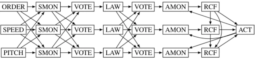
Figure 1: Shuffled, triple channel architecture
interpretationtechnique in cooperation. Briefly outlined, the approach consists first in an abstract inter-pretation pass to discover coarse bounds on the numerical state variables of the system; ak-induction engine and our lemma generation techniques are then ran in parallel to search for potential invariants in order to strengthen the property. We insist on the fact that the primary goal of the proposed method is discovering missing information needed to prove properties the verification of which is either very ex-pensive or impossible with currently available methods and tools, rather than improving the performance of the verification of properties which are already relatively easily provable.
The paper is structured as follows: Section2describes the embedded software architectures targeted by our work. Related work and tools are discussed in Section 3 before notations and vocabulary are given in Section 4. A description of the underlyingk-induction engine assumed in this paper follows in Section5. We introduce and motivate our approach in Section 6 and detail the lemma generation techniques in Section7. The proposed approach is then illustrated on a reconfiguration logic example and on Rockwell Collins industrial triplex sensor voter in Section8. Implementation is briefly discussed in Section9, before concluding in Section10.
2
Fault Tolerant Avionics Architectures
We consider embedded reactive software functions which contribute to the safe operation of as-semblies of hardware sensors, networked computers, actuators, moving surfaces,etc. calledfunctional chains. A functional chain can for instance be in charge of "controlling the aircraft pitch angle", and must meet both qualitative and quantitative safety requirements depending on the effects of its failure. Effects are ranked from MIN (minor effect) to CAT (catastrophic effect, with casualties). For instance, the fail-ure of a pitch control function is ranked CAT, and the function shall be robust to at least a double failfail-ure and have an average failure rate of at most10−9 per flight hour. In order to meet these requirements, engineers must introduce hardware and software redundancy and implement several fault detection and reconfiguration mechanisms in software.
A frequently encountered architectural design pattern, triplication with shuffle, is depicted in Fig.1. It allows to recover from single failures and to detect double failures. Data sources, data processing hard-ware and functions are triplicated to obtain threechannels. The actuator is not replicated. Data is locally monitored right after acquisition/production, but is also broadcast across channels to be checked using triplex voting functions, in order to detect complex error situations. Last, in each channel, depending on the fault state of the channel and the observable behavior of other channels, thereconfiguration logic
decides whether the channel in question must take control of the actuator or on the contrary mute itself. Beinghealthyfor a channel means that no fault has occurred for a sufficient amount of consecutive time
steps to becomeconfirmed.
Previous work by our team addresses the formal verification of control laws numerical stability [24], yet ensuring proper behavior ofvoting functionsandreconfiguration logicas introduced here is equally
soft-ware. For the voting logic, we focus on BIBO properties, “bounded input implies bounded output”, the verification of which is detailed in Section8.2. For reconfiguration logic, which makes an extensive use of integer timers and discrete logic, we focus on bounded liveness properties such as “assuming at most two sensor, network or CPU faults, the actuator must never remain idle for more than N consecutive time units”, the verification of which is addressed in Section8.1.
3
Related Work and Tools
In this section we review the state of the art of verification tools relevant in our application domain,
i.e., of currently available tools and techniques allowing to address synchronous data flow models written
in Lustre. We distinguish two main families of verification approaches.
First, approaches based on abstract interpretation (AI [9]). The tool NBac [15] for instance allows to analyze properties of Lustre models by using a combination of forward and backward fixpoint com-putation using AI. AI tends to need expert tuning for the choice of abstract domains, partitioning,etc.
to behave correctly on the systems we consider. NBac proposes a heuristic selection of AI parameter tuning, which dynamically refines domains and partitionings to try to obtain a better precision without falling in a combinatorial blowup.
Second, the family of k-induction [25] based approaches, with the commercial tool Scade Design
Verifier2, or the academic tool Kind [17]. Kind is the most recently introduced tool, and wraps thek -induction core in an automatic counter example guided abstraction refinement loop whereas the Scade Design Verifier does not.k-induction is an exact technique, in which little or no abstraction is performed
(the concrete semantics of the program is analyzed). Experiments show that it does not scale up out of the box on the systems encountered in our application field. Proving proof obligations on such systems often requires to unroll the system’s transition relation to the reoccurrence diameter of the model which can be very large in practice (hundred or thousands of transitions). For such proof obligations, which are eitherk-inductive for aktoo large to be reached in practice, or even non-inductive at all, numerical lemmas are needed to help better characterize the reachable state space and facilitate the inductive step of the reasoning.
In order to address this common issue with k-induction, automatic lemma generation techniques have been studied. Two main approaches can be distinguished. First, property agnostic approaches, such as [16], in which template formulas are instantiated in a brute force manner on combinations of the sys-tem state variables to obtain a set of potential invariants. They are then analyzed alongside the PO using the maink-induction engine. Second, property directed approaches, such as [6,5], in which the negation
of root states of counterexamples are used as strengthening lemmas, with or without generalization, or are used to guide template instantiation. Also worth mentioning, interpolation [18] yields very inter-esting results in lemma generation but unfortunately to our knowledge no interpolation tool analyzing Lustre code exists.
We consider a lemma generation pass successful when the generated potential invariants allow to prove the original proof objective with a k-induction run with a smallk. Once the right lemmas are
found, the proof can be easily re-run and checked by third partyk-induction tools, an important criterion for industrials and certification organisms. As we will see in the rest of the paper, the lemma generation approach proposed in this paper takes inspiration from all the aforementioned techniques : while some-how brute force in its exploration of the gray state space partitionings, our approach discovers relevant lemmas thanks to its property-directed nature.
4
Notations
Let us now define several notions used throughout this paper. First, atransition systemis represented
as a tuplehv,D,I(v),T(v,v′)iwherevis a vector of state variables,Dspecifies the domain of each state variable, either boolean, integer or real valued, I is the initial state predicate, and T is the transition predicate in which v′ represents next state variables. The logic used to express predicates is Linear
Integer or Real Arithmetic with Booleans. The usual notions of trace semantics and reachability are used. Given a formulaPO(v)representing a Proof Objective (PO), we say that the PO holds if no state
ssuch that¬PO(s)can be reached fromI through repeated application ofT. Lustre or Scade programs
can be cast into this representation using adequate compilers.
Anatomis a Boolean or its negation, or a linear equality or inequality in LRA or LIA. Apolyhedron
is a conjunction of atoms. More precisely, we will say polyhedron for not necessarily closed polyhedron, meaning that we do not impose restrictions on the form of the inequalities besides linearity. Theconvex hullof two polyhedra p1andp2is the smallest polyhedron such that it contains p1and p2. We will say
that the convex hullhof two polyhedrap1andp2isexactif and only ifh=p1∪p2, and call it theExact Convex Hull(or ECH) ofp1andp2if it exists. For the sake of clarity, convex hulls that are not necessarily
exact will be calledInexact Convex Hulls(or ICH). Note that for integer variables, the uniqueness of the convex hull is not guaranteed if non-integer values for the coefficients are not forbidden. We ban them in the rest of this paper; in our implementation, it is prevented by the type system. Still, there are several ways to represent the same inequality,e.g. n>0 andn≥1. Despite their difference in representation, these polyhedra enclose the same (integer) points geometrically speaking, so this does not hinder our approach. Convex hull comparison in this paper does not rely on their syntax nor semantics, but rather on the source of the hull, i.e. the original polyhedra used to create them. This will be discussed in Section7during the explanation of our main contribution, thehullificationalgorithm.
5
Proofs by Temporal Induction
The Stuff framework provides an SMT-basedk-induction module. Performing ak-induction analysis of a potential state invariantPon a transition systemhI,Ti consists in checking the satisfiability of the
Basek(I,T,P) andStepk(T,P)formulas, defined in (1), for increasing values ofk, starting from a user specifiedk>1.
Basek(I,T,P)≡
Initial state
z }| {
I(s0) ∧
trace of k-1 transitions
z ^ }| {
i∈[0,k−2]
T(si,si+1)∧
Pfalsified on some state
z _ }| {
i∈[0,k−1] ¬P(si)
Stepk(T,P)≡
^
i∈[0,k−1]
T(si,si+1)
| {z }
trace ofktransitions
∧ ^
i∈[0,k−1]
P(si)
| {z }
Psatisfied on firstkstates
∧ ¬P(sk) | {z } Pfalsified by last state
(1)
The base and step instances are analysed, until either a base model has been found, in which case the proof objective is falsified, a user specified upper bound forkhas been reached for base and step, in
which case the status of the proof objective is still undefined, or ak value has been discovered so that both formulas are unsatisfiable, which proves the validity of the objective.
• elementsP∈Fnare such thatBasen(I,T,P)is satisfiable: they areFalsified;
• elementsP∈Unare such thatBasen(I,T,P)is unsatisfiable andStepn(T,P)is satisfiable: they are
Undefinedbecause neither falsifiable norn-inductive;
• elements ofVnare such thatBasen(I,T,VP∈VnP)is unsatisfiable andStepn(T,
V
P∈VnP)is
unsatis-fiable: they are mutuallyn-inductive,i.e. Validon the transition system.
6
Approach Overview: Backward Exploration and Hull Computation
Our lemma generation heuristic builds on a backward property-directed reachability analysis. We use Quantifier Elimination (QE [19,22,3]) to compute successive preimages of the negation of the PO, in the spirit of [21,10]. In our approach, the states characterized by the preimages are generated in a way such that(i)they satisfy the PO and(ii)from them, it is possible to reach a state violating the PO
if certain transitions are taken. Such states will be referred to asgray states. This can be achieved by
calculating the preimages as follows:
preimage1=QE(s′,PO(s)∧T(s,s′)∧ ¬PO(s′))
preimagei=QE(s′,PO(s)∧T(s,s′)∧preimagei−1[s′/s]) (fori>1)
(2)
whereQE(~v,F)returns a quantifier-free formula equisatisfiable to∃~v,F and such thatFV(QE(v,F)) =
FV(F)\v. The preimages themselves are assumed to be in DNF, by using [19] as a QE engine for
instance.
From these preimages we extract information using two search heuristics introduced and motivated in the rest of this section and detailled in Section7. These heuristics run in parallel, alongside the backward analysis computing the next preimage and ak-induction engine. The backward analysis is not run to a fixed point before proceeding further, it is rather meant to probe the gray state space around the negation of the PO, and feeding the potential lemma generation with the preimages as soon as they are produced. To extract information out of the preimages, at any point of the backward exploration, their dis-junction is considered: it represents the gray states found so far as a union of polyhedra. The main idea underlying the potential lemma generation is to explore the ways in which those polyhedra can be grouped using convex hull calculation, thus discovering linear relations over state variables representing boundaries between convex regions of the gray state space. Since these convex boundaries enclose unau-thorized states, they are negated before being sent to ourk-induction engine to check their validity and
try to stenghten the PO.
The PO is successfully strengthened by a set of lemmas when the setVk of valid POs, produced by thek-induction analysis detailled in Section5, contains the main PO at the end of a run. If the original
PO is not strengthened by the potential invariants extracted from the currently available preimages, a new preimage is calculated, bringing more information. Yet, when the PO is strengthened and proved valid, it can be the case that not all elements of the valid subsetVkare needed to entail the original PO. A minimization pass inspects them one by one, discardingl6=POfromVk ifV(V\l)remainsk-inductive, to obtain a relatively small and readable set of lemmas.
Note that, in the backward exploration, the choice of which variables to eliminate by QE and which to keep is important. Eliminating the next state variables and keeping the current state variables is not satisfactory in the general case, as on large scale systems, many state variables might not be relevant for the PO under investigation, and might hinder the performance of the convex hull calculation ork
influence of the PO, in theircurrent state version. In particular, the system inputs are eliminated since
they do not provide more information from a backward analysis point of view.
x y
0 1 2 3 4 0
1 2 3
s1 s2
s3
s4
s5
(a) ECH on integers
x y
0 1 2 3 4
0 1 2
s1 s2
(b) ECH on Reals
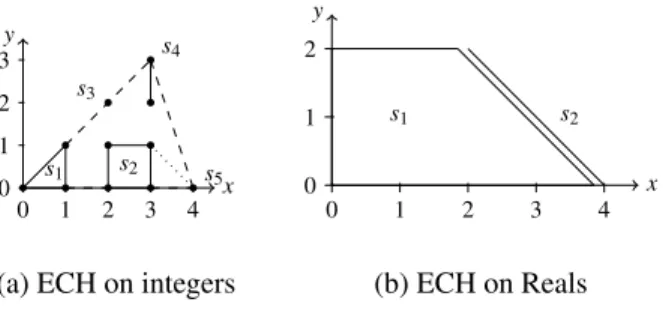
Figure 2: New relations with hulls Before going into the details of the
po-tential lemma generation algorithm, let us il-lustrate how computing ICHs and ECHs can actually make new numerical relations ap-pear, using the examples given in Figure2a
and Figure2b.
In Figure 2a, the gray state space of a system with two integer state variables is represented. States are represented as dots, polyhedrons1 contains three states,
polyhe-dras3ands5only contain one stateetc.
Computing exact convex hulls over these base polyhedra in the LIA fragment yields (at least) two new borders,i.e. potential relational invariants, pictured as dashed lines. An example of merging order
is to merges1withs2,s3withs4,{s1,s2}with{s3,s4}, and{s1,s2,s3,s4}withs5(1).
On a system with real valued state variables however, as shown in Figure2b, the only case in which we willdiscovera new border by computing exact convex hulls is when one is the limit of another, as illustrated on Figure2b. Heres1is made of 0≤x, 0≤y≤2 andy+x−4<0;s2is made of 0≤y≤2 andy+x−4=0, so the resulting hull will be 0≤x, 0≤y≤2 andy+x−4≤0. The information learned this way has little chance of strengthening the PO.
As will be seen in the next sections, when trying to discover new relations, ECH-based techniques work best for integer valued systems, while ICH can be beneficial for both real or integer valued systems.
6.1 A First Example
x y
0 1 2 3 4 5 6 7 8 9 10 0 1 2 3 4 5 6
(1) (2)
Figure 3: ECH calculation on the double counter We consider a simple example called the
dou-ble counter3with two integer state variablesxand
yand three boolean inputsa,bandc. Variablesx
andyare initialized to 0, and are both incremented
by one whenais true or keep their current value
whenais false. The variablexis reset ifb∨cis true, and saturates at nx. The variable y is reset when c is true and saturates at ny, hence y can-not be reset without resettingx, andnx>ny. The proof objective isx=nx⇒y=ny. Here is a pos-sible transition relation for such a system:
T(s,s′) = if(b∨c) thenx′=0 else if(a∧x<nx) thenx′=x+1 elsex′=x
∧ if(c) theny′=0 else if(a∧y<ny) theny′=y+1 elsey′=y
.
Let us see now how the proposed approach performs on this system when fixingnx =10 andny= 6 for instance. First, using the abstract interpretation tool presented in [23], bounds on x and y are easily discovered: 0≤x≤nx=10 and 0≤y≤ny=6, yet the PO cannot be proved with AI without further manual intervention. So, using these range properties oncek-induction has confirmed them, we
start the backward property-directed analysis, which outputs a first preimage: x=9 ∧ 0≤y<5(1).
(a) Two inputs voter, first preimage (b) Two inputs voter with ICH
Figure 4: Simple voting logic.
Unsurprisingly, it is too weak to conclude, i.e. its negation is not k-inductive for a smallk. The next preimage isx=8 ∧ 0≤y<4 ∨x=9 ∧ 0≤y<5(2) which does not allow to conclude either for the same reason. Instead of iterating until a fixed point is found, consider the graph on Figure 3. It shows the two first preimages as dashed lines which seem to suggest a relation betweenxandy, pictured as a bold line. This relation can be made explicit by calculating the convex hull of the disjunction of the first two preimages – since this particular system can stutter, it is the same as(2). This yields 8≤x≤9∧0≤y<x−4. Note that this convex hull is an ECH, since bothxandyare integers. The four inequalities are negated – they characterize gray states – and are sent to thek-induction engine. Potential
invariants¬8≤x,¬x≤9 and¬0≤yare falsified, and the PO in conjunction with lemma¬y<x−4 is found to be 1-inductive.
In fact, this PO could also be proved correct byk-induction given the bounds found by AI only, by unrolling the transition relation to the reoccurrence diameter of the system. In practice, even on such a simple system it is not possible for large values ofnx andny (hundreds or thousands of transitions). The performance of our technique on the other hand is not sensitive to the actual value of numerical constants: it will always derive the strengthening lemma from the first two preimages. Obviously, the time needed to compute the preimages is not impacted by changing the constants values either.
For more complex systems with preimages made of more than two polyhedra, simply merging them in arbitrary order using convex hull calculation is not robust since the resulting convex hulls would depend on the merging order, and interesting polyhedra could be missed. This idea of an exhaustive enumeration of the intermediary ECHs that can appear when merging a set of polyhedra is explored in Section7.1.
6.2 A Second Example
Let us now consider briefly a two input, real valued voting logic system derived from the Rockwell Collins triplex voter. We will not discuss the system itself since the triplex voter is detailled in Sec-tion8.2. It simply allows us to represent graphically the state space in a plan. The PO here is that two of the state variables,Equalization1andEqualization2, range between−0.4 and 0.4. Figure4depicts
the corresponding square. On Figure4awe can see the first preimage calculated by our backward reach-ability analysis as black triangles, and the strengthening lemmas found by hand in [11] transposed to the two input system as a gray octagon. Calculating ECH on this first preimage does not allow to conclude.
A more relevant approach would be to calculate ICH. Yet, since the ICH of all the preimage polyhedra is the [−0.4,0.4]2 square, we need to be more subtle and introduce a criterion for ICH to be actually
satisfiability test performed using a SMT solver. This check allows us to identify overlapping areas of the gray state space and to over-approximate them, while not merging disjoint areas in the gray state space explored so far. This approximation obtained through ICH resembles widening techniques used in abstract interpretation [9] in the sense that it allows tojumpforward in the analysis iterations, yet it
differs in the sense that, contrary to widening, it does not ensure termination. The only goal here is to generate potential invariants for the PO, and Figure4shows that the ICH yields exactly the dual, in the [−0.4,0.4]2square, of the octagon invariant found by hand in [11]. This second idea of using ICHs to
perform overapproximations will be discussed in Section7.4.
7
Generating Potential Lemmas Through Hull Computation
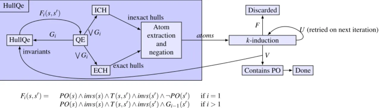
We now detail two heuristics which use the preimages output by the backward analysis. The first one follows the example from Section 6.1 and consists in a thorough, exact exploration of the parti-tionings of the gray state space. After explaining the basic algorithm in Section7.1, optimizations are developed in Section 7.2. A small example illustrates the method in Section7.3. The second heuris-tic over-approximates areas of the gray state space in the spirit of the discussion in Section6.2, and is discussed in Section7.4. Both aim at discovering new relations between the state variables which once negated become potential invariants. Figure6provides a high level view of the different components and the way they interact internally and with the exterior.
7.1 Hullification Algorithm
The algorithm presented in this section, calledhullification, calculates all the convex hulls that can be created by iterating the convex hull calculation on a given set of polyhedra, called thesource poly-hedra. In this algorithm we will calculate ECH as opposed to ICH to avoid both losing precision in the process and the potential combinatorial blow up – ICH are used in a different approach in Section7.4. The difficulty here is to not miss any of the ECH that can be possibly calculated from the source poly-hedra. Indeed, back to the example on Figure2a the merging order(1)misses the ECH of s2 ands5
(represented as a dotted line), and consequently the potential relational lemmay≤ −x+4, which could have strengthened the PO.
Imperative and slightly object-oriented pseudo-code is provided on Algorithm 1. The purpose of
generatorSetMemoryis related to optimizations, discussed in Section7.2. Please note that for the sake
of clarity, the function called on line 20 is detailed separately on Algorithm2. The hullification algorithm iterates on a set of pairs called thegeneratorSet: the first component of each of these pairs is a convex
hull called thepivot. The second one is a set of convex hulls the pivot will be tried to be exactly merged
with, called the pivotseeds. Note that since the ECHs are calculated by merging polyhedra two by two, our hullification algorithm cannot find convex hulls that require to merge more than two polyhedra at the same time to be exact.
The generatorSet is initialized such that for any couple(i,j) such that 0≤i≤nandi< j≤n, pi is a pivot and pj is one of its seeds, line 3. AnewgeneratorSet is initialized with the same pivots as the
generatorSet but without any seeds (line 8). At each iteration (line 6), a first loop enumerates the pairs
of pivot and seeds of the generation set (line 9). Embedded in the first one, a second loop iterates on the seeds (line 11) and tries to calculate the ECH of the pivot and the seed (line 14) as described in Section4. If the exact merge was successful, the new ECH is added to the seeds of the pivots of the
Algorithm 1Hullification Algorithm:
hulli f ication({pi|0≤i≤n}).
1: generatorSetMemory={{pi}|0≤i≤n} 2: sourceMap={pi→ {pi}|0≤i≤n}
3: generatorSet={(pi,Si)|0≤i≤n∧Si={pk|i<k≤n}}
4: generatorSetMemory=generatorSetMemory∪ {{pi,pj}|0≤i≤n,i<j≤n} 5: f ixedPoint=false
6: while(¬fixedPoint)do
7: f ixedPoint=true
8: newGeneratorSet={(pi,{})|∃S,(pi,S)∈generatorSet} 9: for all((pivot,seeds)∈generatorSet)do
10: sourcePivot=sourceMap.get(pivot)
11: for all(seed∈seeds)do
12: sourceSeed=sourceMap.get(seed)
13: source=sourcePivot∪sourceSeed
14: hull=computeHull(pivot,seed)
15: newGeneratorSet.update(pivot,newGeneratorSet.get(pivot)−seed)
16: if(hull6=false)then
17: f ixedPoint=false
18: sourceMap.add(hull→source)
19: newGeneratorSet=
20: updateGenSet(hull,source,pivot,seed,newGeneratorSet)
21: end if
22: end for
23: end for
24: generatorSet=newGeneratorSet
25: // Communication. 26: end while
27: return{pi|∃S,(pi,S)∈generatorSet}
Algorithm 2Updating thenewGeneratorSet:
updateGenSet(hull,source,newGeneratorSet). 1: result={}
2: for all((pivotAux,seedsAux)∈newGeneratorSet)do
3: sourceAux=sourceMap.get(pivotAux)
4: shallAdd= (sourceAux∪source)6∈generatorSetMemory&&
5: (sourceAux6⊂source)
6: if(shallAdd)then
7: result.update((pivotAux,seedsAux∪ {hull}))
8: generatorSetMemory.add(sourceAux∪source)
9: else
10: result.add((pivot,seeds))
11: end if
12: end for
13: result.add((hull,{}))
14: returnresult
generatorSethave all been inspected and if new ECH(s) have been found, a new iteration begins with the
newGeneratorSet. When no new convex hulls are discovered during an iteration, the algorithm returns
all the ECHs found so far (line 27).
7.2 Optimizing Hullification
The hullification algorithm is highly combinatorial, and this section presents optimizations that im-prove its scalability.
elements of this set can be redundant, in the sense that the new hulls derived from them, if any, would be the same even though the elements are different. The key idea to reducing redundancy is to keep a link between any ECH calculated and the source polyhedra merged to create it, thereafter called the ECH source, and use this information to skip redundant ECH calculation attempts.
Consider for example Figure5a. If we already tried to merge the ECH of source{s1,s2,s3}with the
one of source{s4,s5}then it is not necessary to consider trying to merge say the ECH of source{s3,s4}
with the one of source{s1,s2,s5}. The result would be the same,i.e.the same ECH or a failure to merge
the convex hulls exactly (the same ECH here). Note that since we are generating all the existing ECHs from the source polyhedra, this case happens every time an ECH can be calculated by merging its source in strictly more than one order, that is to say veryoften. More generally, we do not want to attempt merges of different hulls deriving from the same set of source polyhedra.
s1s2 s3 s4
s5
(a) Square example
s1 s3 s2
s4 s5
(b) Hat example
Figure 5: Hullification redundancy issues Another source of redundancy is that, when a seed
is added to a pivot during the generatorSet update, it represents a potential merge of the union of the pivot source and the seed source. Even if this merge has not yet been considered, a potential merge of the same source might have already been added to the
generatorSet through a different seed added to a dif-ferent pivot. In this case we do not want the seed to be added. So, in order to prevent redundant elements
from being added to thegeneratorSet, we introduce a memory calledgeneratorSetMemory, and con-trol how new hulls are added to thenewGeneratorSet. For a new hull to be added to a pivot as a seed,
source(pivot)∪source(hull)6∈generatorSetMemorymust hold (Algorithm2line 4); if the hull is indeed
added to the seeds of the pivot, thengeneratorSetMemory+ =source(pivot)∪source(hull)(Algorithm2
line 8). Informally, this memory contains the sources of all the potential merges added to the generator set. This ensures that the merge of a source will never be considered more than once, and that the merges we did not consider were not reachable by successive pair-wise ECH calculation.
Also, we forbid adding a seed to a pivot’s seeds if the source of the latter is a subset of the former, since the result would necessarily be the seed itself (we call this(1)). Another improvement deals with
whenhullification interacts with the the rest of the framework. Since our goal is to generate potential
invariants, we do not need to wait for the hullification algorithm to terminate to communicate the potential invariants already found so far. They are therefore communicated, typically tok-induction, after each big iteration of the algorithm (loop on Algorithm 1line 25). This has the added benefit of launching k-induction on smaller potential invariant sets.
There is a drawback in comparing hulls using their sources: assume that two of the input (source) polyhedrapiandpjare such thatpi⇒pj. Then the exact merge ofpiandpjsucceeds and yields the hull of source{pi,pj}, which is reallypj. As a consequence, the pivots of thegeneratorSet are redundant, as are their seeds and in the end the merge attempts. To avoid this, we first check the set of input polyhedra and discard redundant ones.
Last but not least, merges are also memorized in between calls to the algorithm so that we do not call the merge algorithm when considering two polyhedra we already merged during a previous call. Since hullification is called on the ever-growing disjunction of all preimages found so far, each new disjunction contains the previous one and this represents a significant improvement.
7.3 Hullification Example
Let us now unroll the algorithm on a simple example depicted on Figure5b. For the sake of con-cision a source{s1,s2,· · ·,sn}will be written 12· · ·n. We write generator sets in the following fashion: {(pivot,[seeds])}.
With this convention, the initial generatorSet is {(1,[2,3,4,5]),(2,[3,4,5]),(3,[4,5]),(4,[5]),(5,[])}. ThenewGeneratorSet for the firstbig stepiteration trace is as follows:
1,[] 2,[] 3,[] 4,[] 5,[]
1,[] 2,[13] 3,[] 4,[13] 5,[13] 13,[]
1,[] 2,[13] 3,[] 4,[13,23] 5,[13,23] 13,[] 23,[]
1,[45] 2,[13,45] 3,[45] 4,[13,23] 5,[13,23] 13,[45] 23,[45] 45,[]
At firstnewGeneratorSetis the same asgeneratorSet without seeds (first line of the trace). We first consider 1 as a pivot. The merge of 1 and 3 works while the other ones fail, leading to the second line of the trace. Note that 13 is not added to 1 nor 3 since 1⊆13 and 3⊆13 by (1). With this pivot we add three sources to thegeneratorSetMemory: 213, 413 and 513(2). The next pivot is 2 which is merged with 3 while the merges with the other seeds fail. After thenewGeneratorSetupdate we obtain the third line of the trace. Note that 23 is not added to the seeds of 1 since source 213 has already been added to thegeneratorSetMemoryat(2)so 23∪1∈generatorSetMemory. Similarily, it is not added to the seeds of 13 either. Next pivot 3 cannot be merged with any of its seeds. Pivot 4 can be merged with 5 producing the fourth line of the generator trace. A new big step iteration begins during which 2 will be merged with 13 and 3 with 45 while all the other merges will fail. At the beginning of the third big step iteration thegeneratorSetis
{(1,[345]),(2,[345]),(3,[]),(4,[123]),(5,[123]),
(13,[345]),(23,[345]),(45,[123]),(123,[345]),(345,[])}.
No new hull is found and the algorithm detects that a fixed point has been reached.
7.4 Another Way to Generate Potential Invariants: ICHs
As mentioned before in Section7.1, ECH calculation cannot do much for real state variables. We therefore propose a second approach based on Inexact Convex Hull (ICH) calculation modulo intersec-tion as menintersec-tioned in Secintersec-tion6.2, simply called ICH calculation in the rest of this paper. That is, two polyhedra will be inexactly merged if and only if their intersection is not empty. This regroups areas of the gray state space that are not disjoint and over-approximates them to make new numerical relations appear. An efficient way to check for intersection is to check the satisfiability of the conjunction of the constraints describing the two polyhedra using an SMT solver. Note that this technique is also of interest in the integer case.
For a given set of polyhedra more ICHs than ECHs can be created, in practice often a lot more. The hullification algorithm using ICHs thus tends to choke. We propose the following algorithm, only briefly described for the sake of concision.
HullQe
Fi(s,s′) = PO(s)∧invs(s)∧T(s,s′)∧invs(s′)∧ ¬PO(s′) ifi=1
PO(s)∧invs(s)∧T(s,s′)∧invs(s′)∧G
i−1(s′) ifi>1
HullQe QE
ICH
ECH
Atom extraction
and negation
k-induction Discarded
Contains PO Done
Gi
Fi(s,s′)
W Gi
WG
i
inexact hulls
exact hulls
atoms U(retried on next iteration)
F
V
invariants
Figure 6: High level sequential description
Although the intermediary ICHs computed in this algorithm depends on the order in which the pivots are selected and merged with the other polyhedra, its result does not. Indeed, the fact that two polyhedra have a non-empty intersection will stay true even if one or both of them are merged with other polyhedra. This result, as depicted in Section6.2, is an over-approximation of disjoint areas of the gray state space. In practice, both the ECH based hullification and the ICH calculation heuristics run in parallel, and the sets of potential invariants they output are merged before being sent to thek-induction. This allows us to combine the precision of ECHs with the over-approximation effect of ICHs. A high level view of our approach is available on Figure6. The next section will present two examples taken from a functional chain as presented in Section2 each illustrating the ideas introduced in this section: a reconfiguration logic system and a voting logic system.
8
Applications
In this section we discuss the results of the proposed approach on two real world examples: a recon-figuration logic and the triplex voter of Rockwell Collins.
8.1 Reconfiguration Logic
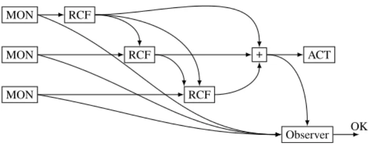
Distributed reconfiguration logic as presented in Section2would be best described as a distributed priority mechanism. In each redundant channel, the reconfiguration logic comes last and monitors the warning flags raised by the monitoring logic implemented earlier in the data flow. Integer timers and latches are used to confirm warnings over a number of consecutive time steps and trigger a reconfigura-tion. The duration of the various confirmations can vary from a few steps to hundreds or thousands of steps and are tuned by system designers to be not overly sensitive to transient perturbations, which would unnecessarily trigger reconfigurations of otherwise healthy channels, while being fast enough to ensure safety. Assuming at most two sensors, network or CPU faults, the following generic property is expected to hold for the reconfiguration mechanism: “No unhealthy channel shall be in control for more thanN
steps”. This property can be decomposed and instantiated per channel. However, a property such as “No more than one channel shall be in command at any time”, or “The actuator must never stay idle for more thanm4steps” are more challenging because they cover all three channels simultaneously and drag many
MON
MON
MON
RCF
RCF
RCF
+ ACT
Observer OK
Figure 7: Reconfiguration subsystem with observer.
the absence of control of the actuator has been confirmed for the requested amount ofm4 consecutive
steps. The proof objective on the system/observer composition is to show that the output of this observer can never be true.
The timer logic found in this system is similar to that of the toy example developed in Section6.1, and instantiated several times, indeed a channel becoming corrupt triggers several timers with different bounds, running into each other or in parallel. Let us now see how hullification performs on this system. The first preimage does not contain enough information, since hullification generates no potential lemma which either strengthens the PO or isk-inductive by itself. The union of the first and second
preim-ages however allows hullification to generate about 200 potential invariants. Once they are negated,
k-induction invalidates most of them and indicates the PO was found (1-)inductive conjoined with about 50 lemmas after about 30 seconds of computation.
After the minimization phase described in Section6, it turns out that only three lemmas are required. If we calltimeri the integer variable used to count the time channeliis not in command for 1≤i≤3, andtimero the timer used by the observer, the lemmas are: ¬(timero−timeri ≥m4−mi−1) where 1≤i≤3. These lemmas are found no matter the values of themifor 1≤i≤4. We insist on the interest of hullification here. Merging polyhedra in some single arbitrary order is too coarse and the resulting hull cannot strengthen the PO, whereas the thorough exploration generates useful lemmas.
The reconfiguration logic was also analyzed using NBac, Scade Design Verifier and Tinelli’s Kind. NBac did not succeed in proving the property after 1 hour of computation. Both the Scade Design Verifier and Kind kept on incrementing the induction depth without finding a proof after 30 minutes of run time. The invariant generation of Kind was also run on this system, and yielded a number of small theo-rems, but obviously not property directed and unfortunately not sufficient to strengthen the PO and prove it.
In conclusion, the proposed combination of backward analysis, hullification andk-induction allows
us to complete a proof in a few seconds on a widely used avionics design pattern, where other state of the art tools fail. In addition, we see two very interesting points worth highlighting about hullification:
(i)The PO is made (1-)inductive, implying the proof can easily and quickly be re-run and checked by
any existing induction tool;(ii)the time needed to complete the proof does not depend on the numerical values of the system –about thirty seconds on a decent machine in practice for this system4. This is very important for critical embedded systems manufacturers as point(i) means that the proofs are
trustwor-thy, both for the industrials themselves and the certification organisms. On the other hand, point(ii)
implies that strengthening lemmas can be very quickly generated for similar design patterns with altered numerical values, easing the integration of formal verification in the development process. Indeed, it
avoids the need for an expert to manually transpose the lemmas on the new system, as can be the case for complicated and resource/time consuming proofs.
8.2 The Triplex Voter
Let us now turn to the Rockwell Collins triplex sensor voter, an industrial example of voting logic as introduced in Section2, implementing redundancy management for three sensor input values. This voter does not compute an average value, but uses themiddleValue(x,y,z) function, which returns the input value, bounded by the minimum and the maximum input values (i.e. zify<z<x). Other voter
algorithms which use a (possibly weighted) average value are more sensitive to one of the input values being out of the normal bounds. The values considered for voting areequalizedby subtracting equaliza-tion values from the inputs. The following recursive equaequaliza-tions describe the behaviour of the voter with
X∈ {A,B,C}:
EqualizationX0 = 0.0
EqualizedXt = InputXt−EqualizationXt
EqualizationXt+1 = 0.9∗EqualizationXt+
0.05∗(InputXt+ ((EqualizationXt−VoterOut putt)−Centeringt))
Centeringt = middleValue(EqualizationAt,EqualizationBt,
EqualizationCt)
VoterOut putt = middleValue(EqualizedAt,EqualizedBt,EqualizedCt)
The role of the equalization values is to compensate offset errors of the sensors, assuming that the middle value gives the most accurate measurement.
We are interested in proving Bounded-Input Bounded-Output (BIBO) stability of the voter, which is a fundamental requirement for filtering and signal processing systems, ensuring that the system out-put cannot grow indefinitely as long as the system inout-put stays within a certain range. In general, it is necessary to identify and prove auxiliary system invariants in order to prove BIBO stability.
So, we want to prove the stability of the system, i.e. we want to prove that the voter output is bounded as long as the input values differ by at most the maximal authorized deviationMaxDevfrom the true value of the measured physical quantity represented by the variableTrueValue. In our analysis,
we fixed the maximal sensor deviation to 0.2, a value that domain experts gave us as typical value in practical applications. It is staightforward to prove that the system is stable if the equalization values are bounded.
When applied to Rockwell Collins triplex sensor voter, our prototype implementation manages to prove the PO in less than 10 seconds by discovering that−0.9≤∑3i=1Equalizationi≤0.9 is a strength-ening lemma, using ICH calculation. Again, the time taken to complete the proof does not depend on the system numerical constants, and the strengthened PO is (1-)inductive. We insist on the importance of these characteristics for both industrials and certification organisms: the proof is trustworthy and can be redone easily for similar, slightly altered designs.
9
Framework and Implementation
Our actor oriented collaborative verification framework [8] called Stuffis composed of several ele-ments: thek-induction engine, the abstract interpreter, the backward analysis, ICH calculation and ECH
hullification. They can all evolve in parallel and communicate.
Stuff is written in Scala except for the abstract interpreter, written in OCaml. We implemented the backward analysis and the two heuristics presented in this paper using the QE algorithm from [19] modified to handle integers or reals whith booleans. The underlying projections of [19] are performed by the Parma Polyhedra Library [1], also used for convex hull computation. Stuff can use any SMT lib 2.0 [2] compliant solver thanks to the Assumptio5 actor oriented SMT solver wrapper. In practice, the backward analysis and the heuristics use Microsoft Research Z3 [20] and MathSat 5 [14] by the University of Trento.
A run of the framework in the default configuration begins by a preprocessing phase using abstract interpretation with intervals as abstract domains in order to infer bounds on the state variables. This provides an over-approximation of the reachable state space which once verified byk-induction is propa-gated to all the other elements of the framework. The rest of the analysis follows the approach discussed in Section6with the backward analysis feeding preimages to both ECH hullification and ICH calcula-tion. They in turn feed potential invariants to thek-induction engine which detects real invariants and check if they strengthen the property as described in Section6. In this setting, even if our approach does not consider the initial states, it benefits from the over-approximation of the AI preprocessing phase, which takes into account the initial states but not the PO. The AI results also enhance the quality of the output and the overall performance of the incrementalk-induction engine.
10
Conclusion
In this paper, the authors presented two automatic and property directed lemma generation heuristics, which operate on preimages of the negation of the proof objective obtained by a backward exploration, itself powered by quantifier elimination.
The first heuristic originality lies in the thorough exploration of a set of possible convex partitionings of the gray state space by exact convex hull calculations. This exploration, calledhullification, is per-formed incrementally, as soon as new preimages containing new information about the gray state space, are computed by the backward analysis. As illustrated on the reconfiguration logic example, the blowup inherent to the exploration of the partitionings is avoided thanks to the optimizations discussed in this paper and far outperforms other available tools.
The second heuristic over-approximates disjoint areas of the gray state space by accepting inexact hulls when the candidate polyhedra intersect. It performs very well in the Rockwell Collins Triplex Sensor Voter experiments, allowing to conclude a proof none of the other state of the art tools could conclude.
These results, obtained with the prototype implementation of the proposed method, are of interest in our application field. Indeed, they allow to discover strengthening lemmas, in reasonable time, for essential safety properties of widely used fault tolerance design patterns at model level, a task which has proved difficult to achieve using other techniques such as AI ork-induction with manual analysis of failed proofs.
Future work include further reflexion on systems mixing integers and reals and on heuristics us-ing preimages from the backward analysis. Also, the authors think that when hullification cannot find strengthening lemmas, it can still provide interesting starting points for template based techniques and experiments have been started in this direction. Outside of the proposed approach, the authors believe in a multi method approach and will continue to experiment in this direction: work on an implementation of PDR [5,13] adapted to numerical systems is in progress. It was observed that PDR is able to discover range lemmas similar to those found using interval based AI, while being able to conclude inductive proofs, and the cooperation of hullification and PDR is being studied. The long term goal is to refine and bridge the verification techniques developed for precise parts of the functional chains (voting, reconfig-uration logic and numerical stability for control laws) to obtain a methodology and tool support suitable for end-to-end verification of avionics software at model level.
References
[1] R. Bagnara, P. M. Hill & E. Zaffanella (2008): The Parma Polyhedra Library: Toward a Complete Set of Numerical Abstractions for the Analysis and Verification of Hardware and Software Systems. Science of Computer Programming72(1–2), pp. 3–21. Available at http://doi.acm.org/10.1016/j.scico. 2007.08.001.
[2] C. Barrett, A. Stump, C. Tinelli, S. Boehme, D. Cok, D. Deharbe, B. Dutertre, P. Fontaine, V. Ganesh, A. Griggio, J. Grundy, P. Jackson, A. Oliveras, S. Krsti´c, M. Moskal, L. de Moura, R Sebastiani, T. D. Cok & J. Hoenicke (2010):C.: The SMT-LIB Standard: Version 2.0. Available athttp://citeseerx.ist.psu. edu/viewdoc/summary?doi=10.1.1.190.4897.
[3] N. Bjørner (2010): Linear Quantifier Elimination as an Abstract Decision Procedure. In J"urgen Giesl & Reiner H"ahnle, editors:Automated Reasoning,Lecture Notes in Computer Science6173, Springer Berlin / Heidelberg, pp. 316–330. Available athttp://dx.doi.org/10.1007/978-3-642-14203-1_27. [4] B. Blanchet, P. Cousot, R. Cousot, J. Feret, L. Mauborgne, A. Miné, D. Monniaux & X. Rival (2003): A
Static Analyzer for Large Safety-Critical Software. In:Proceedings of the ACM SIGPLAN 2003 Conference on Programming Language Design and Implementation (PLDI’03), ACM Press, San Diego, California, USA, pp. 196–207. Available athttp://dx.doi.org/10.1145/781131.781153.
[5] A. R. Bradley (2011): SAT-Based Model Checking without Unrolling. In: VMCAI, pp. 70–87. Available at
http://dx.doi.org/10.1007/978-3-642-18275-4_7.
[6] A. R. Bradley & Z. Manna (2006): Verification Constraint Problems with Strengthening. In: ICTAC, pp. 35–49. Available athttp://dx.doi.org/10.1007/11921240_3.
[7] P. Caspi, D. Pilaud, N. Halbwachs & J. Plaice (1987): Lustre: A Declarative Language for Programming Synchronous Systems. In: POPL, pp. 178–188. Available at http://doi.acm.org/10.1145/41625. 41641.
[8] A. Champion, R. Delmas, P.L. Garoche & P. Roux (2011):Towards Cooperation of Formal Methods for the Analysis of Critical Control Systems. In: SAE Int. J. Aerosp., pp. 850–858. Available athttp://dx.doi. org/10.4271/2011-01-2558.
[9] P. Cousot & R. Cousot (1977): Abstract Interpretation: A Unified Lattice Model for Static Analysis of Programs by Construction or Approximation of Fixpoints. In: POPL, pp. 238–252. Available at
http://doi.acm.org/10.1145/512950.512973.
[11] M. Dierkes (2011): Formal Analysis of a Triplex Sensor Voter in an Industrial Context. In G. Salaün &
B. Schätz, editors:Proceedings of the 16th edition of FMICS,LNCS6959, Springer, pp. 102–116. Available athttp://dx.doi.org/10.1007/978-3-642-24431-5_9.
[12] M. Dierkes & D. Kästner (2012):Transferring Stability Proof Obligations from Model Level to Code Level. Available athttp://www.erts2012.org/Site/0P2RUC89/5C-1.pdf.
[13] N. Een, A. Mishchenko & R. Brayton (2011): Efficient Implementation of Property Directed Reachability. Available athttp://dl.acm.org/citation.cfm?id=2157675.
[14] A. Griggio (2012): A Practical Approach to Satisfiability Modulo Linear Integer Arithmetic. JSAT8, pp. 1–27. Available athttp://jsat.ewi.tudelft.nl/content/volume8/JSAT8_1_Griggio.pdf. [15] B. Jeannet (2003): Dynamic Partitioning in Linear Relation Analysis: Application to the Verification of
Reactive Systems. Formal Methods in System Design23(1), pp. 5–37. Available athttp://dx.doi.org/ 10.1023/A:1024480913162.
[16] T. Kahsai, Y. Ge & C. Tinelli (2011): Instantiation-Based Invariant Discovery. In M. Bobaru, K. Havelun-dand G. Holzmann & R. Joshi, editors: Proceedings of the 3rd NASA Formal Methods Symposium (Pasadena, CA, USA), Lecture Notes in Computer Science 6617, Springer, pp. 192–207. Available at
http://dl.acm.org/citation.cfm?id=1986326.
[17] T. Kahsai & C. Tinelli (2011): PKind: A parallel k-induction based model checker. In: PDMC, pp. 55–62. Available athttp://dx.doi.org/10.4204/EPTCS.72.6.
[18] Kenneth L. McMillan (2008):Quantified Invariant Generation Using an Interpolating Saturation Prover. In:
TACAS, pp. 413–427. Available athttp://dx.doi.org/10.1007/978-3-540-78800-3_31.
[19] D. Monniaux (2008): A Quantifier Elimination Algorithm for Linear Real Arithmetic. In: LPAR, pp. 243– 257. Available athttp://dx.doi.org/10.1007/978-3-540-89439-1_18.
[20] L. M. de Moura & N. Bjørner (2008):Z3: An Efficient SMT Solver. In:TACAS, pp. 337–340. Available at
http://dx.doi.org/10.1007/978-3-540-78800-3_24.
[21] L. M. de Moura, H. Rueß & M. Sorea (2003):Bounded Model Checking and Induction: From Refutation to Verification (Extended Abstract, Category A). In:CAV, pp. 14–26. Available athttp://doi.acm.org/10. 1007/978-3-540-45069-6_2.
[22] T. Nipkow (2010): Linear Quantifier Elimination. J. Autom. Reasoning 45(2), pp. 189–212. Available at
http://dx.doi.org/10.1007/s10817-010-9183-0.
[23] P. Roux, R. Delmas & P.L. Garoche (2010):SMT-AI: an Abstract Interpreter as Oracle for k-induction.Electr. Notes Theor. Comput. Sci.267(2). Available athttp://dx.doi.org/10.1016/j.entcs.2010.09.018. [24] P. Roux, R. Jobredeaux, P.L. Garoche & E. Féron (2012): A generic ellipsoid abstract domain for linear
time invariant systems. In: Proceedings of the 15th ACM international conference on Hybrid Systems: Computation and Control, pp. 105–114. Available athttp://doi.acm.org/10.1145/2185632.2185651. [25] M. Sheeran, S. Singh & G. Stålmarck (2000):Checking Safety Properties Using Induction and a SAT-Solver.