LAND USELAND COVER CHANGE AND ITS IMPACT ON SOIL EROSION PROCESS IN BEGNAS TAL RUPA TAL WATERSHED USING GEOSPATIAL TOOLS, KASKI DISTRICT, NEPAL

(1)

i

LAND USE/LAND COVER CHANGE AND ITS IMPACT ON

SOIL EROSION PROCESS IN BEGNAS TAL RUPA TAL

WATERSHED USING GEOSPATIAL TOOLS, KASKI

DISTRICT, NEPAL

(2)

ii

LAND USE/LAND COVER CHANGE AND ITS IMPACT ON

SOIL EROSION PROCESS IN BEGNAS TAL RUPA TAL

WATERSHED USING GEOSPATIAL TOOLS, KASKI

DISTRICT, NEPAL

Dissertation Supervised By Professor Pedro Cabral, Ph.D

Dissertation Co-Supervised By Professor Edzer Pebesma, Ph.D

Professor Filiberto Pla, Ph.D

(3)

iii

ACKNOWLEDGEMENTS

I would like to express my deep appreciation to the European Union an Erasmus Mundus Program for giving me an opportunity to learn master program in Geospatial Technologies and its application. I acknowledge my sincere thanks to Prof. Dr. Marco Painho, Director ISEGI, University of NOVA to do my master research work and other external support.

I‟m deeply grateful to my supervisor Prof. Dr. Pedro Cabral, ISEGI for his serious and patient guidance, encouragement, understanding and inspiration, without which this project would not have been completed. I am equally grateful to my co-supervisors Prof. Dr. Edzer Pebesma, Prof. Dr. Filiberto Pla and Dr. Pedro Latorre for their guidance and encouragement.

I wish to express my foremost gratitude to Prof. Dr. Werner Kuhn, Dr. Christoph Brox, IFGI, Prof. Dr. Joaquin Huerta and Prof. Dr. Michael Gould UJI for providing all the facilities and other help for executing this thesis and master program successfully.

I am equally thankful to all the staff member of UJI, IFGI and ISEGI family. I want to extend my sincere thanks to Dolores Apanewicz, UJI, Caroline Wahle, IFGI, Maria do Carmo and Olivia, ISEGI, for their great help during stay at Spain, Germany and Portugal.

(4)

My gratitude is equally to all staff members of ISEGI library and whole Lumiar Residence Family for their help during the different stage of my thesis work.

I would also like to express my sincere to all the Officers and Staff members of Forest Department, Soil Conservation Department and Metrology Department of Kaski District, Nepal. I would like to thank Mr. Basanta Raj Gautam for his help. Last but not least I would like to thanks all my Geospatial Technologies classmates.

(5)

v

LAND USE/LAND COVER CHANGE AND ITS IMPACT ON

SOIL EROSION PROCESS IN BEGNAS TAL RUPA TAL

WATERSHED USING GEOSPATIAL TOOLS, KASKI

DISTRICT, NEPAL

ABSTRACT

(6)

KEYWORDS

GIS

Land Use Change

Mountain

Soil Erosion

(7)

vii

ACRONYMS

ANSWERS – Areal Non-Point Source Watershed Environment Response Simulation

AGNPS – Agricultural Non-Point Source Pollution Model CBS – Central Bureau of Statistics

CF – Community Forest

DDC – District Development Committee FAO – Food Agriculture Organization

ILWIS – Integrated Land and Water Information System LUCC – Land Use Land Cover Change

SLEMSA – Soil Loss Estimation Equation for Southern Africa USLE – Universal Soil Loss Equation

(8)

INDEX OF TABLES

Table 1: Literature Review on Land Use/Land Cover Change ... 14

Table 2: Literature Review on Soil Erosion ... 16

Table 3: Satellite Data Used for the Study ... 16

Table 4: Hardware Used for Study ... 17

Table 5: Software Used for Study ... 17

Table 6: Land Use/Land Cover Classification Scheme for Mapping ... 20

Table 7: Slope Classes Used in the Study ... 22

Table 8: Aspect Classes Used in the Study ... 23

Table 9: Altitude Class Used in the Study ... 24

Table 10: Input parameters and their weights for pressure zone mapping ... 27

Table 11: Input Parameters (Morgan et. al. 1995) for soil erosion modeling ... 28

Table 12 (a-c): Attribute Values assigned for creating input layers in soil erosion modeling ... 30

Table 13: Annual Rainfall (mm) in Begnas Tal Rupa Tal Watershed, Pokhara, ... 36

Table 14: Minimum Temperature of Begnas Tal Rupa Tal Watershed, Pokhara, Nepal ... 37

Table 15: Maximum Temperature of Begnas Tal Rupa Tal Watershed, Pokhara, Nepal ... 37

Table 16: Area Statistics of Land Use/Land Cover Map of Watershed (November 1988) ... 38

Table 17: Area Statistics of Land Use/Land Cover Map of Watershed (December 1999) ... 39

Table 18: Area statistics of Land use land cover change from major land use to different land uses in Begnas Tal Rupa Tal Watershed ... 41

Table 19: Area statistics of Soil Erosion of Begnas Tal Rupa Tal Watershed, 1988 43 Table 20: Area statistics of Soil Erosion of Begnas Tal Rupa Tal Watershed, 1999 44 Table 21: Change area data of Soil Erosion (1988 – 1999) ... 45

Table 22: Area of Pressure Index Map ... 46

(11)

xi

INDEX OF FIGURES

Figure 1: Location of the Study Area ... 5

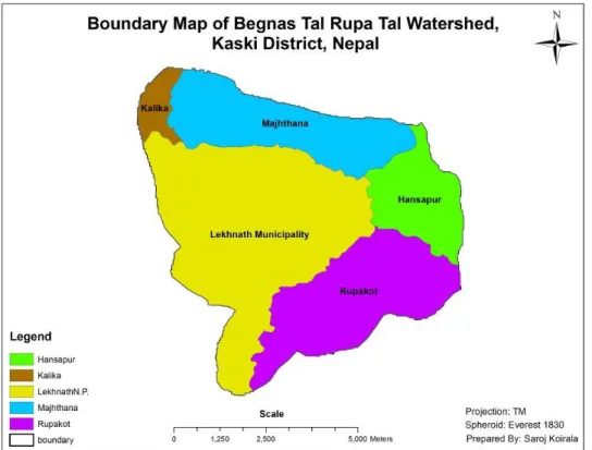
Figure 2: Boundary Map of Begnas Tal Rupa Tal Watershed ... 8

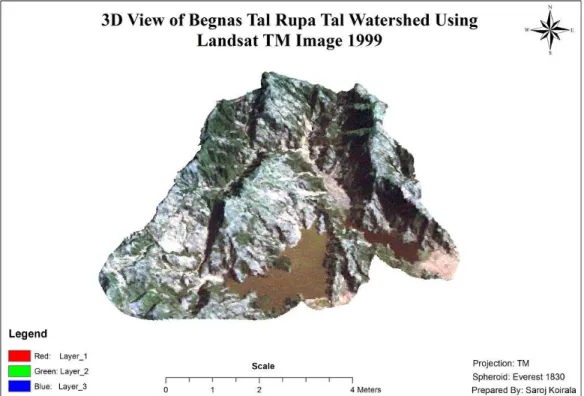
Figure 3: 3D View of Begnas Tal Rupa Tal Watershed ... Error! Bookmark not defined. Figure 4: Road Network of Watershed ... 21

Figure 5: Slope Map of Watershed ... 22

Figure 6: Aspect Map of Watershed ... 23

Figure 7: DEM of Watershed ... 24

Figure 8: Methodology in Land Use/Land Cover Map Preparation ... 25

Figure 9: Methodology to detect Land Use/Land Cover Change from 1988-1999 ... 26

Figure 10: Soil Erosion Modeling (Revised Morgan-Morgan-Finney-Model) ... 34

Figure 11: Drainage Map of Begnas Tal Rupa Tal Watershed ... 35

Figure 12: Land Use Land Cover Map of Watershed ... 38

Figure 13: Land Use/Land Cover Map of Watershed ... 39

Figure 14: Land Use/Land Cover Change Map (1988-1999) ... 40

Figure 15: Soil Erosion Map of Begnas Tal Rupa Tal Watershed ... 43

Figure 16: Soil Erosion Map of Begnas Tal Rupa Tal Watershed ... 44

(12)

1

1. INTRODUCTION

1.1 Background

The high intensity of land use and the fast rate of change in land cover are the characteristic features of developing countries whose economy is based on primary production. The human impacts upon land are very high because of increasing human population. The land use land cover is defined as the observed physical layer including natural and planted vegetation and human constructions, which cover the surface of the Earth. A watershed is a structural and functional unit of a landscape consisting of various environments and sustaining a certain biodiversity. Land Use Land Cover Change (LUCC) around the world has been altering natural ecosystem. Land use from a watershed perspective, is a watershed characteristics influenced by human activities and plays a significant role in delivering sediment and modified water yield (quantity, quality and regime) in the river. Due to anthropogenic activities, the Earth surface is being significantly altered in some manner and man‟s presence on the Earth and his use of land has had a profound effect upon the natural environment thus resulting into an observable pattern in the land use/land cover over time. The land use/land cover pattern of a region is an outcome of natural and socio– economic factors and their utilization by man in time and space. Land is becoming a scarce resource due to immense agricultural and demographic pressure.

The land use/land cover pattern of a region is an outcome of natural and socio – economic factors and their utilization by man in time and space. Hence, information on land use / land cover and possibilities for their optimal use is essential for the selection, planning and implementation of land use schemes to meet the increasing demands for basic human needs and welfare. This information also assists in monitoring the dynamics of land use resulting out of changing demands of increasing population. Knowledge of land cover and land use change is important for many planning and management activities (Lillesand and Kiefer, 1994).

(13)

2

spread and health of the world‟s forest, grassland, and agricultural resources has become an important priority. Viewing the Earth from space is now crucial to the understanding of the influence of man‟s activities on his natural resource base over time. In situations of rapid and often unrecorded land use change, observations of the earth from space provide objective information of human utilization of the landscape. Over the past years, data from Earth sensing satellites has become vital in mapping the Earth‟s features and infrastructures, managing natural resources and studying environmental change.

Remote Sensing (RS) and Geographic Information System (GIS) are now providing new tools for advanced ecosystem management. The collection of remotely sensed data facilitates the synoptic analyses of Earth - system function, patterning, and change at local, regional and global scales over time; such data also provide an important link between intensive, localized ecological research and regional, national and international conservation and management of biological diversity.

Satellite data interpretation followed by field verification from several time points allows the creation of land cover maps over greater spatial extents and more frequent time steps (Nagendra, 2001). Because these classifications are spatially explicit, they not only provide information on percent changes in land cover, but also allow for evaluation of the spatial location of these changes and their association with environmental and biophysical landscape parameters that may be critical associates of this change (Nagendra et. al., 2004).

1.2 Statement of the Problem

Watershed management has become an increasingly important issue in many tropical countries including Nepal as government agencies and non-governmental groups struggle to find appropriate management approaches for improving production of natural resource systems. Principles, concepts and approaches related to watershed management have experienced a vast change during the past few years but yet there is no universal methodology for achieving effective watershed management (Naiman

(14)

conflict of increasing population, resource degradation and resource depletion (Joshi

et al., 2001). Over exploitation of watershed resources by the growing population has resulted in its degradation in the most parts of the world (FAO, 1985). Watershed conditions have been further deteriorating due to improper land use practices such as deforestation, uncontrolled and excessive grazing, use of unsuitable land for agriculture, and infrastructure development. The degradation in watershed conditions has severely affected the natural resources base of the country. Accelerating pressure on forests and agricultural lands for meeting the basic human needs of fuel, fodder and food have resulted in forest and farmland degradation. Resources are the basis of human beings‟ living and development, while these are limited. After a period of depletive exploitation, the speedy vanish of forest, the degradation of the land, the shortage of energy and its consequential impact on the micro as well as global environment not only decreases the living standard of human beings but also threat to their development and survival.

In Nepal forestry and land use change alone contribute about 85% of national account of greenhouse gases emission. Total CO2 emission from land use change and

forestry sector in 1994 was about 8.1 million tones. Involvement of wide range of stake-holder‟s interest objectives and needs makes the process complex and multidimensional in nature. These complexities necessitate a systematic approach to find out the proper utilization techniques and sustainable management plans. This study attempts to analyze Land use Land cover change and its impact on Soil Erosion process in Begnas Tal Rupa Tal Watershed using geospatial tools. Some of the potent questions related to research problems are as follows:

What are the drivers for the changes in land use land cover occurred during the years 1988 and 1999?

What is the impact of forest resource utilization pattern on soil erosion process?

(15)

4 1.3 Objectives of the Study

This study attempts to analyze land use land cover change and its impact on soil erosion process by applying and adopting commonly used satellite remote sensing and GIS techniques at Begnas Tal Rupa Tal Watershed in Nepal. Specific objectives of the study are set as follows:

To prepare land use/land cover maps using satellite data; To create spatial and non-spatial database of the area of study;

To detect land use/land cover changes based on 1988 and 1999 satellite; imageries; and

To prepare soil erosion map by analyzing changing impacts of resource utilization on soil erosion process.

1.4 Organization of the study

(16)

2. STUDY AREA

2.1 The Study Area

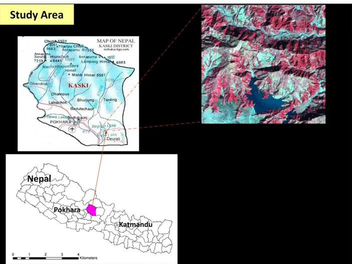
The Begnas Tal Rupa Tal Watershed is located between 28˚07'30"N to 28˚18'00"N latitudes and 84˚00'00"E to 84˚20'00"E longitudes covering 50.94 km2 area of Kaski District in western Nepal (Fig.1). The land use practice in watershed can be characterized a semi agricultural watershed in mid-hill belt (600-1420 meter) of a mountain ecosystem. It is rich in biodiversity on the one hand and represents mountain characteristics in the Nepal Himalayas on the other. The elevation ranges from 600 meter to 1420 meter which has provided habitat of sub-tropical species of vegetation.

(17)

6 2.2 Land Use

Forest, agriculture, open forest and barren lands are the main land use categories of the Begnas Tal Rupa Tal Watershed. The forest land use basically consists of community forestry whereas agriculture land use consists of field crop cultivation. The most common gregarious natural vegetation types under tropical to sub tropical monsoon climates are Schima wallichii, Castonopsis indica, Alnus nepalensis and Shorea robusta (Department of Forest, 2002). However, the watershed is interspersed by a number of patches of rural settlement and agricultural fields. Agricultural lands are allotted to wet and dry crops cultivation depending upon prevailing local climatic conditions.

2.3 Livestock

Raising livestock is an important economic activity in the watershed area. In spite of the time involved in collecting fodder and looking after the livestock and other social costs, raising livestock is profitable. Livestock is also the main source of manure for improving soil fertility and of draft power for plugging. The availability of forest and water resources encourages the farmers to raise livestock.

2.4 Socio-economic conditions

The watershed inhabitants are of many ethnic groups and castes and practice Hinduism, Buddhism and Islam. Due to economic, social and ecological pressures, the local people are forced to leave their villages for short and long-term employment. The lower castes often work as seasonally paid lab ours. A socio-economic study carried out in 1990 indicated that about 2% of the population was landless, and that 60% of the farmers own less than one hectare of land. Only an average of 3.8% own above 1 ha of cultivated land (Poudel, 1985).

2.5 Natural Vegetation

(18)

2.6 Climate

The climate of the watershed varies from tropical to sub-tropical monsoon types depending upon the altitude. Local convection hailstorms in autumn and strong winds during the dry spring are the limiting factors to certain crops. The seasonal cycle is cool-warm and dry winter and warm-hot and wet summer. The agricultural activity conforms to the seasonal rhythm and the vagaries of monsoon affect the farmer‟s poverty or prosperity (Gurung, 1965).

2.7 Sunshine

Begnas Tal Rupa Tal Watershed Area gets nearly six hours sunshine on an average round the year. The minimum hour is found in June when monsoon cloud covers the entire sky. Until September the sunshine hours slowly increase indicating the cloud stay for shorter period before the precipitation (Sharma 1975).

2.8 Wind

Wind is one of the important climatic parameter. In general wind is not very strong with average annual wind speed of 2.2 km per hour. Moreover south-west north-east and south-east winds also blow in the valley.

2.9 Evapotranspiration

The minimum evaporation is 2 mm/per day in January and maximum is 6.2 mm in May and June. The gap between evaporation and monthly precipitation is not much. But watershed areas lies in the city area being porous like honey-comb structure the percolation rate is abnormally high; hence a wide gap is created between the water requirement and water available for the plants.

2.10 Location and Extent

(19)

8 2.11 Ecosystem Condition

The Begnas Tal Rupa Tal Watershed has different ecosystems viz., aquatic, wetland and terrestrial ecosystems. The aquatic ecosystem constitutes two distinct zones: Limetic (deep open water central zone) and littoral (shallow depth peripheral / shoreline zone). The wetland ecosystem consists of swampland and marshlands located along the floodplain. The terrestrial ecosystem consists of different land use types: forest grazing land and agricultural land. Urban and rural settlements are located along Lake Shoreline and gentler hill slopes as well. Villages are interspersed into agricultural lands. The common species include Schimia wallichii, Castonopsis indica, Alnus nepalesnsis, Shorea robusta, Bombax ceiba and Ficus spp.

economically important and commercially threatened species under IUCN Red data book include: Swerita chirayita, Bergenia ciliata, Choreospondias axillares, Elaeocarpus sphaericus.

(20)

(21)

10

3. METHODOLOGY

3.1 Introduction

Land use land cover change and its impacts on soil erosion process is an explanatory type of research. The database is generated from the satellite images and published and unpublished records supported by primary data obtained from field observation and household survey. Geometry and topology of landforms pattern of forest resource uses and change in land use/land cover (1988 to 1999) and soil mapping are designed as the dimensions of spatial analysis.

3.2 Conceptual Construct

Begnas Tal Rupa Tal Watershed area is very rich in forests and species diversity. Different kinds of herbs and shrubs are found in this study area. Forest based small industries can be developed in these areas particularly where these forests are found. The term watershed is not restricted to surface water run-off but includes interactions with sub-surface water. Ecologically a watershed is a mosaic interacting abiotic components viz., soil, land, topography, climate, and biotic component viz., flora and fauna. The functions and values provided by natural features are included in the development of a watershed system. Administrative boundaries such as a block, village, town, city, district, and country are part of a watershed where the size of the watershed or basin in each case becomes a determining factor. Therefore, it helps in any conservational, economical and developmental activities to be planned and managed ensuring long-term sustainability.

3.3 Studies in Land Use/Land Cover Change

(22)

S.N. Studies in Land Use/Land Cover Change 1.

2.

3.

4.

Khanal and Bastola (2005) studied land use/land cover changes in Phewa Lake Watershed where watershed area has changed drastically due to opening of highways and urban facilities of sub-metropolitan Pokhara city. They found that most of the changes have occurred on agricultural land, forest area and built-up-area and minor changes have been found in different land cover. The study shows that land use change is a continuous process of change from one aspect to another aspect. The natural factors and human beings are the major agents for the change in cultural landscapes of nay region of the country. Finally they conclude that the country should develop an integrated land use policy for the overall economic and environmental development.

Chaudhary et al. (2008) studied land use/land cover changes in Northern Part of Gurgaon District, Haryana, India and found that there is tremendous pressure on the natural resources due to increasing population, maximum increase in the area under settlements, which has increased almost four times over this period. The wasteland has also decreased drastically due to its conversion to settlements and other categories. The expansion of Gurgaon City is due to increasing population and Industrial/Infrastructural development pressure of National Capital, as Guragon is the most preferred and favorable destination.

Tiwari (1999) studied land use changes in Indian Himalaya. The rapid growth of population has brought about extensive land-use changes in the region, mainly through the extension of the Himalayan watersheds through reduced groundwater recharge, increased run-off and soil erosion.

(23)

12

S.N. Studies in Land Use/Land Cover Change

5.

6.

7.

changes in natural resource management practices and the resulting land use patterns.

Weng, Q., (2001) used satellite remote sensing, GIS and stochastic modeling to find out land use change analysis in the Zhujiang, his results indicated that there has been a notable and uneven urban growth and a tremendous loss in cropland between 1989 and 1997. The land use change process has shown no sign of becoming stable. The technologies of satellite remote sensing, GIS and stochastic modeling are combined to address land use and land cover changes in the Zhujiang Delta, China, during the period 1989-1997. It was found that urban or built-up land and horticulture farms have notably increased in area, while cropland has decreased. The integration of satellite remote sensing, GIS, and Markov modeling provides a means of moving the emphasis of land use and land cover change studies from patterns to processes.

Giri et al., (2001) analyzed the multi-temporal and multi-seasonal NOAA AVHRR Satellite data of 1985/86, and 1992/2000 in Continental Southeast Asia to prepare historical land cover maps and to identify areas undergoing major land covers transformations (called “hot spots”). The identified “hot spots” areas were investigated using high-resolution satellite data such as Landsat and SPOT supplemented by intensive field survey. Shifting cultivation, intensification of agricultural land were found to be the principal reasons for land use land cover change in Oudomxay provience of lao P.D.R, Mekong Delta of Vietnam and Loei provience of Thailand respectively. The rapid rate of economic development, demographics and poverty are believed to be the underlying forces responsible for the change in this region.

(24)

8.

9.

10.

11.

12.

pastures land to agriculture. However, some areas revealed an opposite trend where previously agriculture areas were afforested.

Pfaff (1999) combined aggregated forest cover change from remote sensing data and included both population and economic variables in his analysis of deforestation in the Amazon. The major empirical finding was the importance of land characteristics (soil quality and vegetation density) and factors affecting transportation costs (distance to markets and own and neighboring county road networks) in determining deforestation rates. Pereira (2004) grouped the possible causes for land use change into two categories: a) real changes in land cover; b) differences observed due to other factors. It includes occurrence of floods and population growth. He suggested the changes induced by the growth of settlements can have different origins like the excessive utilization of natural fuel wood, cattle overgrazing or conversion of land to agriculture.

Xiaomei Y. and Rong Qing L.Q.Y., (1999) noted that information about change is necessary for updating land cover maps and the management of natural resources. The information may be obtained by visiting sites on the ground and or extracting it from remotely sensed data.

Barret et al. (2009) carried out case study of carbon fluxes from land change in the Southwest Brazilian Amazon and found land change is responsible for one-fifth of anthropogenic carbon emissions. In Brazil, three-quarters of carbon emissions originate from land change. They produced land-cover maps of pasture, forest, and secondary growth from 1993, 1996, 1999, and 2003 using an unsupervised classification method (overall accuracy = 89%). They presents new methods for estimating emissions reductions from carbon stored in the vegetation that replaces forests (e.g., pasture) and sequestration by new (> 10-15 years) forests, which reduced gross emissions by 16%, 15% and 22% for the period of 1993-1996, 1996-1999 and 1999-2003 respectively.

(25)

14

13.

14.

Brazil and found rubber tapping plays a less important role in livelihood strategies, as welfare is linked to non-extractive activities. Households pursue diverse livelihood activities including extractives, small-scale market cultivation, animal rearing, and cattle production. The overall results suggest that land use/land cover change is highly dynamic in the reserve.

Millette et al. (1995) examined three villages in the Kathmandu valley of Nepal for pathways to criticality, which they define as a regional situation in which the rate or extent of environmental degradation precludes the continuation of current human use systems or levels of human well being, given feasible adaptations and societal capabilities to respond. They conclude that despite the difficulties of analyzing remote sensing imagery in a mountainous area where high slope angles and shadows complicate image analysis, remote sensing imagery in combination with ground-based data can "provide information highly germane to the analysis of changing nature society relations, including trajectories toward endangerment and criticality."

Gautam et al. (2003) provided important insights into the dynamics that occurred in forested area and other major land use of the Upper Koshi Watershed in between 1976 and 2000 and provides a solid quantitative foundation for forest policy and institutional analysis.

Table 1: Literature Review on Land Use/Land Cover Change

3.4 Studies on Soil Erosion

(26)

Equation for Southern Africa (Stocking, 1981) was developed in Zimbabwe on the basis of the USLE model. There are some other models such as ANSWERS (Areal Non-point Source Watershed Environment Response Simulation, Beasley et.al., 1980), and AGNPS (Agricultural Non-Point Source Pollution Model, Young et.al., 1987), these models are based on grid cells and were developed to estimate runoff quality, with primary emphasis on sediment and nutrient transport. Although USLE has been widely used through various modified versions, its application in mountainous terrain with steep slopes is still questionable. Some models, such as AGNPS or ANSWER, may not be suitable in the Nepalese context because of very high data demand and AGNPS in particular is not adapted well enough to the Nepalese mid-hill belt mountain conditions (Kettner, 1996). Considering all these, the model developed by Morgan, Morgan and Finney (Morgan et al., 1984) is used in the present study to assess soil loss from hill slopes in the mid-hill belt of Nepal. Due to its simplicity, flexibility and strong physical base it was selected.

S.N. Studies on Soil Erosion

1.

2.

Awasthi et al. (2002) have carried out accurate measurement of land use/land cover and watershed analysis based on GIS in Mardi and Phewa Lake Watershed using aerial photographs of 1978 and 1996. In these watersheds there was a net increase in forest cover with a corresponding decrease in shrub and rain-fed agriculture. A significant area under agriculture in 1978 was found abandoned in 1996 in both watersheds most likely due to increased out migration of the labour force.

(27)

16

S.N. Studies on Soil Erosion

3.

variables and land-use change as the response variable. They analyzed that based on the logistic model, it is anticipated that cereal cultivation in western Lesvos will probably be abandoned in the near future.

Shrestha (1997) He analyzed that soil erosion is a crucial problem in Nepal where more than 80% of the land area is mountainous and still tectonically active. Results provided by running Morgan Morgan and Finney model in a GIS environment show that annual soil loss rates are the highest (up to 56 tonnes/ha/yr) in the areas with rain fed cultivation, which is directly related to the sloping nature of the terraces. The lowest soil losses (less than 1 tonne/ha/yr) are recorded under dense forest. In the degraded forest, the soil loss varies from 1 to 9 tonnes/ha/yr and in the grazing lands it is estimated at 8 tonnes/ha/yr. Erosion rates are higher on the south facing sub watershed than on the north facing one. Finally, his study shows that soil erosion can be modeled in the mountainous region.

Table 2: Literature Review on Soil Erosion

3.5 Materials

The study is based on both remote sensing and ancillary data. The details of different hardware and software used during analysis and field observations are given below.

Details Used

The details of satellite data used in study are given table 3.

Table 3: Satellite Data Used for the Study Data

Used Path/Row

Spatial Resolution (m)

Spectral Resolution (µm)

Spectral Bands

Used (µm) Band

Swath (km)

Date of Acquisition

Landsat

TM 142/040

30

Band 1: 0.450 - 0.515

Band 1: 0.450 -

0.515 Blue

185 December 13, 1999 & November 20, 1988 Band 2: 0.525 -

0.605

Band 2: 0.525 -

0.605 Green Band 3: 0.630 -

0.690

Band 3: 0.630 -

0.690 Red

Band 4: 0.760 - 0.900

Band 4: 0.760 -

0.900 NIR

Band 5: 1.550 - 1.750

Band 5: 1.550 -

1.750 SWIR

120 Band 6: 10.40 -

12.5 Band 6: 10.40 - 12.5

Thermal IR

30 Band 7: 2.080 -

(28)

Ancillary Data

Topography sheet developed by department of survey Nepal is used in present study. Scale is 1:25,000 (Sheet No. 2884: 13A 13B). Same as Land Systems Map of scale 1:50000 (Sheet No. 62 P/15, 62 P/16) is used developed by department of survey Nepal. Socio-economic data from household survey as well as from Village Secretary and District Development Cooperation. Community forest operational plan from District Forest Office (DFO) Kaski. Annual Report of Nepal Agriculture Research Council (NARC). District Profile Kaski district, Nepal. Meteorological data from Department of Meteorology and Demographic data of the Central Bureau of Statistics Nepal.

Instruments / Field Equipments

Global Positioning System Garmin 12 Channel, Magnetic Rangers compass, Binocular, Camera are used for collecting data in field.

Ground Truth Data

Field Performa: It was designed to collect the ground data (Annexure 1). Hardware

The computer hardware used during the study is given table 4.

Hardware Uses

Laptop hp (4 GB RAM) Data storage, software and internet support. Plotter To print hardcopy, paper maps and poster. Scanner To convert pictures or maps to digital form.

Printer

To produce high quality hardcopy, computer output viz. literature, thesis and report.

Table 4: Hardware Used for Study

Software

The software used in the study is in table 5.

Software Uses

Arc View GIS 3.2a Digitizing Mapping

ERDAS IMAGINE

9.1

Registration and processing of topographic map and satellite data change detection Image Classification

Arc Info 8.0 Topology (cleaning and building)

ILWIS 3.3 Academic Morgan Morgam Finney Soil erosion modelling

Microsoft office Data entry Non-Spatial Data Analysis Thesis Compilation and

Presentation

Arc Map To Prepare Map Composition

(29)

18 3.6 Methods

The total research activities were set into pre-fieldwork, fieldwork and post-fieldwork stages. Description of work in each stage is as below:

3.6.1 Pre Field Stage

Pre-field work consisted initiation of project followed by downloading and processing different satellite data and creation of base map. Project planning pre-processing and database creation are major works performed in this stage.

Project Planning

The study was proposed and planned in view of the problems in resource conservation and their sustainable use in Begnas Tal Rupa Tal Watershed of Kaski district, Nepal. On the basis of literature review and the knowledge gained during the study period, it was felt that the remote sensing along with GIS could be useful to detect changes in land use/land cover between 1988 and 1999. Project planning includes

Collection of literature pertaining to the research topic; Study of topographic maps and

Procurement of remote sensing data products followed project planning.

Pre-processing

Pre-processing of data includes radiometric and geometric corrections are made before data base creation. The procedures of corrections are discussed as follows:

Radiometric Correction

(30)

and thus to remove atmospheric effects from visible wavelength data. The corrected radiance values can be related to physical properties such as concentrations of chlorophyll and sediments in the water. The “darkest pixel” technique can also be used in land studies, provided that an area of deep (and hopefully unpolluted) water is available somewhere within the study image.

Geometric Correction

Geometric correction addresses errors in the relative positions of pixels. It is undertaken to avoid geometric distortions from a distorted image. Raw digital image usually contains geometric distortions so significant that they cannot be used as maps. The sources of these distortions range from variations in the altitude and velocity of the sensor platform to factor such as panoramic distortion, earth curvature, atmospheric refraction, relief displacement and non-linear ties in the sweep of a sensor‟s IFOV. To carry out the geometric correction in image which we are going to be used for analysis of the proposed study area. We need to rectify those images with the reference map e.g. corrected topo sheet (Produced by Survey Department of Nepal) map on 1:25,000 scales. For getting better accuracy during geometric corrections common well distributed ground control points necessary. A sub-pixel accuracy of control points was obtained for all satellite images by geo-referencing. The images used were then re-sampled by cubic convolution method. The data sets were then co-registered for further analysis.

3.6.2 Field Work Stage

Entire study area was visited in the month of September 2009. From the field different necessary information was obtained.

Ground Truth Collection

(31)

20

taken from forest department. Based on the preliminary reconnaissance survey and visual interpretation of the satellite data, land use in the study area was classified as below (Table 6):

S.N. Land Use/Land Cover

Description

1. Dense Mixed Forest

Forest composed of trees of two or more species intermingled in the same canopy forming 40-70% dense canopy and consisting at least 20% canopy other than principle species. The main species are Schima wallichii, Castanopsis indica, Alnus nepalensis ,Dendrocalamus hamiltonii, Cinnamomum zeylanicum, Syzygium cumini, Myrica esculenta, Rhus javanica etc.

2. Sal Forest Sal (Shorea robusta) occurs in the tropical belt at an altitude below 1000 meter. Some small area of sal forest occurs in Southern hills.

3. Open Forest Forest consist less than 40% in the canopy composition. 4. Agricultural

Land

In the downstream of study area mainly variety of paddy is growing and irrigation also good but in the upstream of the study area water sources and soil are not good. The major crops are Wheat (Triticum spp.), Paddy (Oryza sativa), Millet Soybean, Maize (Zea mays) etc.

5. Barren Land Without vegetation and agricultural crops, soil is very poor in this land. Almost all the cultivation activity is zero. Most of these lands are unproductive.

6. Settlement Very Dense population with compare to past eleven years. 7. Water Body The land covered under natural drainage system like river

streams as well as manmade linear drainage system like canals (used or unused) and natural or manmade linear reservoir or ponds and lakes.

Table 6: Land Use/Land Cover Classification Scheme for Mapping

Other Data Collection

(32)

Road Network Development

Due to some parts of watershed area located in city there is black road where most of the villages have only village road which is not well constructed. Most of the rural people use these types of village road for their daily livelihood requirements.

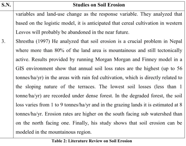
Figure 4: Road Network of Watershed

3.6.3 Post Fieldwork Stage

Preparation of Land Use/Land Cover Map

Procedure of on screen visual interpretation of satellite data was carried out to find out different land use/land cover classes in conjugation with information from maps and ground truth. Land use/land cover map of Landsat TM 1988 image and Landsat TM 1999 image was prepared. The identification and delineation of all classes along with other cover types was done by following the standard visual interpretation technique (Browden and Pruitt, 1983).

Preparation of Slope, Aspect, Drainage and Contour Maps

(33)

22

drainage map was prepared from the same topographic maps. With the help of contours DEM was generated in ArcView GIS 3.2a software. Slope and aspect maps were derived from DEM in same software.

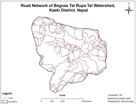
Land Used Cover Map along the Slope

Slope is the gradient of the surface of the ground expressed in either degrees or in percent (Gulati, 1986). Slope plays important role in distribution of land use/land cover. In the present study the slope map is recoded into 5 classes (Table 7). The land use/land cover map was then intersected with slope index map to assess land cover distribution along slope categories.

S.N. Classes Slope (Degree)

1 Flat/almost Flat 0~2 2 Gentle slope 2~6 3 Moderate slope 6~13 4 Moderate to steep slope 13~25 5 Steep slope 25~55

Table 7: Slope Classes Used in the Study

(34)

Land Used Cover Map along the Aspect

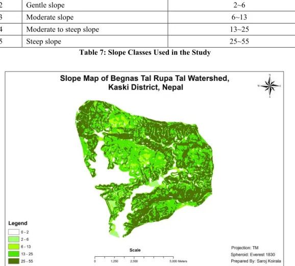
Aspect is the direction towards which the slope faces (Gulati, 1986). The aspect map which was derived from DEM was recorded into 8 classes and each land use/land cover map was intersected with recorded aspect map (Table 8).

S.N. Classes Aspect (Degree)

1 North 0-22.5 337.5-360 2 North-East 22.5-67.5 3 East 67.5-112.5 4 South-East 112.5-157.5 5 South 157.5-202.5 6 South-West 202.5-247.5 7 West 247.5-292.5 8 North-West 292.5-337.5

Table 8: Aspect Classes Used in the Study

Figure 6: Aspect Map of Watershed

Land Used Cover Map along the Altitude

(35)

24

recording in the original DEM. The recorded DEM was then intersected with each land use/land cover map.

Table 9: Altitude Class Used in the Study

Figure 7: DEM of Watershed

S.N. Classes Altitude (Meter)

(36)

25 3.7 Land Use/Land Cover Map Preparation

Figure 8: Methodology in Land Use/Land Cover Map Preparation

Satellite images Landsat TM of 1988 and 1999 are used for land use land cover map, raw images of this year was taken and did radiometric/geometric correction; radiometric correction was done by dark pixel subtraction after that geometric correction. It was done by providing sufficient ground control points in permanent features such as road, canal etc. Preliminary Visual Interpretation was carried out, from topography map boundary was created according to that boundary satellite image was subset. Final interpretation was carried out by sufficient information from ground truth. Finally, land use land cover map was created by digitizing satellite image.

(37)

26

3.8 Land Use Change during (1988-1999) Period

Figure 9: Methodology to detect Land Use/Land Cover Change from 1988-1999

(38)

3.9 Pressure Index Map

It is very essential to find out the areas which are highly on pressure and which are least pressure from resource extraction point of view. Pressure Map has been prepared taking settlement, road and slope index into the consideration. Following table shows the parameters and their respective weights for pressure zone mapping.

Parameters Criteria Weight

Settlement buffer

<200m

0.25 200-400m

>600m

Road buffer

<200m

0.25 200-400m

400-600m

Slope index

<15°

0.50 15-30°

>30°

Table 10: Input parameters and their weights for pressure zone mapping

Pressure index map = 0.5 (slope index) + 0.25 (road buffer) + 0.25 (settlement buffer)

3.10 Soil Erosion Modeling

Revised Morgan Morgan and Finney Model (MMF) with the aid of Remote Sensing and GIS are used in present study. This model was selected because of its simplicity, flexibility and strong physical base. Morgan et al. (1984) presented a simple empirical model for predicting annual soil loss from field-sized areas on hill slopes. The MMF model used the concepts proposed by Meyer and Wischmeier (1969) and Kirkby (1976) to provide a stronger physical base than the Universal Soil Loss Equation (Wischmeier and Smith, 1979).

(39)

28

when erosion is detachment-limited. Thus good information on rainfall and soil is required for successful output (Morgan et al. 1984),

Factor Parameter Definition and remarks

Rainfall R Annual or mean annual rainfall (mm) Rn Number of rain days per year

I Typical value for intensity of erosive rain (mm/h); 10 for

temperate climates 25 for tropical climates and 30 for strongly seasonal climates e.g. Mediterranean type and monsoon

Soil MS Soil moisture content at field capacity or 1/3 bar tension ( w/w) BD Bulk density of the top soil layer (Mg/m³)

EHD Effective hydrological depth of soil (m); depend on vegetation/crop cover presence or absence of surface crust presence of impermeable layer within 0.15 m of the surface.

K Soil detachability index (g/J) defined as the weight of soil detached from the soil mass per unit of rainfall energy.

COH Cohesion of the surface soil (kPa) as measured with a torvane under saturated conditions.

Landform S Slope steepness (°).

Land Cover A Proportion between 0 and 1 of the rainfall intercepted by the vegetation or crop cover.

Et/Eo Ratio of actual (Et) to potential (Eo) evapo-transpiration

C Crop cover management factor; combines the C and P factors of the Universal Soil Loss Equation.

CC Percentage canopy cover expressed as a proportion between 0 and 1 GC Percentage ground cover expressed as a proportion between 0 and 1 PH Plant height (m) representing the height from which raindrops fall from

the crop or vegetation cover to the ground surface

Table 11: Input Parameters (Morgan et. al. 1995) for soil erosion modeling

R = Rainfall; Rn = Number of rainy days per year; I = Intensity of erosive rain (mm/h); MS = Soil moisture content at field capacity (w/w); BD = Bulk Density (Mg/m³); EHD = Effective Hydrological depth of the soil (m); K = Erodibility of the soil (g/J); COH = Cohesion of the surface soil; S = Slope steepness (°); A =

Proportion between 0 and 1 of the rainfall intercepted by the vegetation; Et/Eo = Ratio of actual (Et) to potential (Eo) evao-transpiration; C = Crop cover management factor; CC = Percentage canopy cover; GC = Percentage ground cover; PH = Height of the plant canopy (m).

3.10.1 Soil Erosion Modeling Database Creation Creation of Maps based on Attributes

(40)

maps. Attribute maps of each parameter was created. Finally the erosion model was run in the Integrated Land and Water Information System (ILWIS) a raster based GIS software package capable of combining conventional GIS procedures with image processing and using a relational database (Valenzuela, 1988) applying following steps.

Step1. Estimation of rainfall energy

The procedure for calculating the energy of rainfall is partitioned during interception and the energy of the leaf drainage. The model takes the annual rainfall total (R; mm) and computes the proportion (between 0 and 1) which reaches the ground surface after allowing for rainfall interception (A) to give the effective rainfall (ER):

ER=RA Where,

R = Annual rainfall (mm)

A = Proportion of rainfall which reaches the ground surface after allowing for rainfall interception (according to Morgan it should be between 0 to 1).

(a)

Forest/Land Use Type A GC CC PH Et/E0 C EHD

Dense mixed forest 0.40 0.45 0.45 18.0 0.85 0.004 0.16 Sal Forest 0.38 0.38 0.29 14.0 0.88 0.003 0.18 Open forest 0.20 0.30 0.20 15.0 0.60 0.002 0.13 Agriculture 0.15 0.15 0.15 1.0 0.50 0.002 0.11 Barren land 0.10 0.10 0.05 0.05 0.65 0.001 0.05 Settlement 0 0 0 0 0 0 0 Water body 0 0 0 0 0 0 0

(b)

Rainfall R1988 Rn1988 R1999 Rn1999 I

(41)

30 (c)

Soil Texture MS BD K COH

Fragmental sandy 0.08 1.5 1.2 2.0 Loamy 0.20 1.3 0.8 3.0 Loamy bouldery 0.15 1.2 0.3 2.0 Loamy skeleton 0.10 1.3 0.8 3.0

Table 12 (a-c): Attribute Values assigned for creating input layers in soil erosion modeling

A = Proportion between 0 and 1 of the rainfall intercepted by the vegetation; GC = Percentage ground cover; CC = Percentage canopy cover; PH = Height of the plant canopy (m); Et/Eo = Ratio of actual (Et) to potential (Eo) evao-transpiration; C = Crop cover management factor; EHD = Effective Hydrological depth of the soil (m); R = Rainfall; Rn = Number of rainy days per year; I = Intensity of erosive rain (mm/h); MS = Soil moisture content at field capacity (w/w); BD = Bulk Density (Mg/m³); K = Erodibility of the soil (g/J); COH = Cohesion of the surface soil.

The effective rainfall (ER) is then split into that which reaches the ground surface as direct through fall (DT) and that which is intercepted by the plant canopy and reaches the ground as leaf drainage (LD). The split is a direct function of the percentage canopy cover (CC):

LD = ER CC DT = ER - LD Where,

LD = Leaf drainage ER = Effective rainfall

(42)

The kinetic energy of the direct through fall (KE DT; J/m2) was determined as a function of the rainfall intensity (I; mm/h) using a typical value for the erosive rain of the climatic region i.e.10.

Kinetic energy of the direct through fall was calculated using following standard formula.

KEDT = DT (11.9 + 8.7log I)

Where,

DT = Direct through fall

KEDT = Kinetic energy of the direct through fall (J/m2)

I = Intensity of erosive rain (mm/h) i.e. 15 for subtropical climates (Morgan et. al.; 1995)

The kinetic energy of leaf drainage (KELD; J/m2) is dependent upon the height of the plant canopy (PH; m). Following formula was used to calculate KELD.

KE LD = (15.8 PH0.5) – 5.87 where,

KELD = Kinetic energy of leaf drainage (J/m2) PH = Height of the plant canopy (m)

The total energy of effective rainfall (KE; J/m2 ) was then obtained by summing up KEDT and KELD.

KE = KEDT + KELD

Step 2. Estimation of runoff

(43)

32

capacity (Rc; mm) and that daily rainfall amounts approximate an exponential frequency distribution. The annual runoff is obtained from:

Q = Rexp (-Rc/Ro) where,

Q = Annual Runoff (mm) R = Annual Rainfall (mm)

Rc = Soil moisture storage capacity i.e.1000 MS BD EHD (Et / Eo)

where,

MS = Soil moisture content at field capacity ( w/w) BD = Bulk density (Mg/m3)

EHD = Effective Hydrological depth of the soil (m)

Et/Eo = Ratio of actual (Et) to potential (Eo) evao-transpiration

Ro = Mean rainfall per rain day (R/Rn) where,

R = Annual rainfall (mm)

Rn = Number of rain days per year

Step 3. Soil particle detachment by raindrop impact

In the revised MMF model, rainfall energy can be estimated using rainfall interception. It is therefore, removed from the equation used to describe soil particle detachment by raindrop impact (F; kg/m2) which then simplifies to:

(44)

where,

F = Raindrop impact (kg/m2) K = Erodibility of the soil (g/J)

KE = Kinetic energy of the effective rainfall (J/m2)

Step 4. Soil particle detachment by runoff

Soil particle detachment by runoff was estimated using following formula H = ZQ1.5sinmap (1-GC) 10-3

where,

H = Soil particle detachment by runoff Z = Resistance of the soil i.e. 1/(0.5COH) Q = Annual Runoff (mm)

Sinmap = It was obtained from slope map of the study area by using formula i.e. SIN (DEGGRD) Slope map

GC = Percentage ground cover

Step 5. Transport capacity of runoff

It was calculated by using following formula TC = CQ2 sinmap 10-3

where,

TC = Transport capacity of runoff (kg/m2) C = Crop cover management factor Q = Annual Runoff (mm)

Step 6. Estimation of total annual detachment

(45)

34

where, F = Soil particle detachment by raindrop (kg/m2) H = Soil particle detachment by runoff (kg/m2)

Step 7. Estimation of total annual soil erosion

It was calculated by comparing annual detachment (AD) to annual transport capacity (TC). The lesser of the two values indicates annual soil erosion rate (Meyer and Wischmeier 1969).

Annual Erosion (kg/m2) = if (AD<TC AD TC)

Figure 10: Soil Erosion Modeling (Revised Morgan-Morgan-Finney-Model) Rainfall interception (A)

Canopy Cover (CC) Ground Cover (GC) Conservation Practices (C)

Plant Height (PH) Evapotranspiration Factor (Et/Eo)

Annual Rainfall (R) Rain days (Rn) Erosive Rainfall Intensity (I)

Moisture Content (MS) Bulk Density (BD) Effective Hydrological Depth (EHD)

Detachability Index (K) Soil Cohesion (COH)

Effective Rainfall Energy (K)

Annual Runoff (Q)

Soil Particle Detachment by Raindrop (F)

Soil Particle Detachment by Runoff (H)

Transport Capacity (TC)

Detachment (DE) = F + H

Soil Erosion = mini (DE TC)

Vegetation, Types, Density and Land Use

Map Rainfall Soil Slope

(46)

A = Rainfall interception; CC = Canopy Cover; GC = Ground Cover; C = Conservation Practices; PH = Plant Height; Et/Eo = Evapotranspiration Factor; R = Annual Rainfall; Rn = Rain days; I = Erosive Rainfall Intensity; MS = Moisture Content; BD = Bulk Density; EHD = Effective Hydrological Depth; K = Detachability Index; COH = Soil Cohesion; K = Effective Rainfall Energy; Q = Annual Runoff; F = Soil Practicle Detachment by Raindrop; H = Soil Particle Detachment by Runoff; TC = Transport Capacity; DE = Detachment.

3.11 Hydrology

The source of water for Begnas Tal Rupa Tal watershed is surface water through rivers and rivulets. These are contributed by surface runoff and groundwater recession. There is high density of rivulets. There is both low water table and course texture. Such steep slopes are susceptible to erosion. Lowland area is vulnerable to flood havoc during heavy rains.

(47)

36 3.12 Precipitation

The wet months are July to September, while October to December is dry months. From January the rain starts and the maximum precipitation is received in the month of July. The monsoon starts in mid-June and reaches its maximum intensity in July and falls down slowly in October.

Year January February March April May June July August September October November December

1988 1.6 26.1 73.4 135.6 241.9 782.6 1093.5 810.5 793.9 15 3.6 55

1989 68 14.2 65.5 11.7 518.3 594.1 973.9 871.6 807.2 58.4 44.4 42.9

1990 0 59.6 114.7 44.8 361.1 931.5 732.5 742.5 530.2 99.7 0 2.9

1991 9.9 22.4 77.6 64.2 358.3 497.5 797.7 602.9 994.1 53 0.8 35.2

1992 10.5 24.7 0.5 53.9 247 469.1 793.6 798.7 396.5 246.5 2.4 26.2

1993 9.7 20.2 55.7 205.2 358.4 652.1 965.6 1168.5 478.5 294.7 0.6 0

1994 34.7 49.5 73.2 59.6 380.7 686.9 1020.3 794.4 523.8 97.8 1.8 0

1995 16 43.4 72.5 75.8 282.4 1391.3 1372.1 745.5 560 202.8 80.8 3.9

1996 59.7 75.4 94.6 38.5 371.9 687.5 939.8 857.4 703.4 131.7 0 0

1997 62.5 11.8 45.6 224.6 308.7 545.8 1113.5 604.1 327.4 115.8 30 133.9

1998 0 24.8 107.6 238.9 415.3 769.7 917.2 1493.5 740.3 158.7 9.6 3.4

1999 7 22.6 0 20.6 899.7 979.6 950.5 899.7 730.7 176.4 0 0

Total 279.6 394.7 780.9 1173.4 4743.7 8987.7 11670.2 10389.3 7586 1650.5 174 303.4

Mean 23.3 32.89 65.08 97.78 395.31 748.98 972.52 865.78 632.17 137.54 14.5 25.28

Table 13: Annual Rainfall (mm) in Begnas Tal Rupa Tal Watershed, Pokhara,

Nepal (Source: The Office of the Meteorological Station, Pokhara, Nepal)

3.13 Temperature

(48)

37

1988 8.2 9.7 12.4 16.1 19.3 21.2 22.3 22.2 21.3 16.5 10.2 9.3

1989 6.9 7.4 11.9 14.5 19.1 20.6 21.4 21 20.7 15.9 11 7

1990 8.6 9.3 10.6 15 18.2 21 21.8 21.4 20.6 15.6 11.1 7.6

1991 6.1 8.9 12.6 15.3 19 21.3 22.3 22.1 20.7 16.5 11.2 7.1

1992 7.1 7.9 12.8 15.5 17.2 20.3 21.6 21.9 20.7 16.5 11.2 7.1

1993 8.1 9.8 10.2 14.6 18.5 21.2 22.4 22 20.4 17.4 13.2 8.9

1994 7.4 8.1 14 14.8 18.8 21.4 22.3 22.3 21.4 15.7 9.4 6.4

1995 5.5 6.5 12 15 20 21.9 21.9 22 22.1 17.6 12.1 8.8

1996 7.1 9.4 14.3 15.9 18.1 20.9 22.2 22 20.7 16.5 12.3 7.3

1997 6.2 7.8 12.5 14.5 17.1 20 22.3 22 20.8 14 11.8 7.7

1998 6.8 9.7 11.9 16.3 19.6 22.2 22.6 22.6 21.3 19.3 13.5 8.2

1999 6.5 10.7 13.2 18.7 19.1 20.8 21.7 21.4 21.4 17.4 12.7 9.1

Total 84.5 105.2 148.4 186.2 224 252.8 264.8 262.9 252.1 198.9 139.7 94.5

Mean 7.04 8.77 12.37 15.52 18.67 21.07 22.07 21.91 21.01 16.58 11.64 7.88

Table 14: Minimum Temperature of Begnas Tal Rupa Tal Watershed, Pokhara, Nepal

(Source: The Office of the Meteorological Station, Pokhara, Nepal)

1988 20.4 22.9 25.6 30 30 30.5 29.8 29.4 29.5 28.2 25.3 21.4

1989 18.2 20.9 25.8 30.9 31.2 30.3 28.2 29.9 29.2 28 23.5 19.8

1990 21.3 21 23.7 28.3 29.5 31.2 29.7 30 29.5 27.2 25.5 21.5

1991 19.7 23.9 26.9 29.5 30.1 29.8 30.4 29.9 29.8 28 23.7 20.5

1992 19 19.8 28.3 33.1 29.6 31.3 29.8 30 29.8 26.8 24.3 20.1

1993 18.8 23 25 28.7 29.1 30.4 30.5 29.4 28.1 27 23.7 21.4

1994 19.9 20.7 26.1 29.2 31 30.1 30.5 30.4 28.7 26.9 24.1 20.7

1995 18.7 21.2 26.2 30.4 32.2 29 29.5 30.1 29.5 27.6 23.7 19.8

1996 18.6 21.3 26.6 30.3 31.1 29.3 29.8 29.9 29.3 26.2 24.6 21.7

1997 18.9 20.2 26.4 26.5 29.9 30.4 30.5 30.2 29 25.7 22.9 18.3

1998 18.4 22.1 24.2 28.8 30.5 31.5 29.8 29.2 30 28.6 24.7 21.5

1999 20.6 25.3 29.4 33.6 30 30.1 29.3 29.1 29.9 27.6 24.4 21.5

Total 232.5 262.3 314.2 359.3 364.2 363.9 357.8 357.5 352.3 327.8 290.4 248.2

Mean 19.38 21.86 26.18 29.94 30.35 30.33 29.82 29.79 29.36 27.32 24.2 20.68

Table 15: Maximum Temperature of Begnas Tal Rupa Tal Watershed, Pokhara, Nepal

(49)

38

4. ANALYSIS OF RESULTS AND INTERPRETATION

4.1 Land Use/Land Cover Map using Landsat TM 1988

Land use/land cover map for 1988 is prepared from the Satellite Image of Landsat TM by applying onscreen visual interpretation technique. According to land use/land cover map seven land use classes are identified. Forests and Agricultural Land were dominant land uses in 1988. Proportional share of each land use categories are shown in (Table 17; Fig. 12).

Figure 12: Land Use Land Cover Map of Watershed

S.N. Particulars Area (ha) Percentage 1 Settlement 105.48 2.07 2 Dense Mixed Forest 1756.71 34.48 3 Water Body 394.47 7.74 4 Agriculture Land 1918.71 37.66 5 Sal Forest 14.76 0.29 6 Open Forest 626.76 12.3 7 Barren Land 277.92 5.45

Total 5094.81 100

(50)

4.2 Land Use/Land Cover Map using Landsat TM 1999

Land use/land cover map was prepared of December 1999 Satellite image Landsat TM using onscreen visual interpretation technique. According to land use/land cover map 7 land use classes were identified. In land use/land cover map of Landsat TM 1999 image total area in Settlement 173.84 ha, Dense Mixed Forest 1907.26 ha, Water body 416.07 ha as well as in Agriculture land 2040.99 ha, Sal forest 26.19 ha, Open forest 467.37 ha and Barren land 63.09 ha respectively (Table 18; Fig. 13).

Figure 13: Land Use/Land Cover Map of Watershed

S.N. Particulars Area (ha) Percentage 1 Settlement 173.84 3.41 2 Dense Mixed

Forest 1907.26 37.44 3 Water Body 416.07 8.17 4 Agriculture Land 2040.99 40.06 5 Sal Forest 26.19 0.51 6 Open Forest 467.37 9.17 7 Barren Land 63.09 1.24

Total 5094.81 100

(51)

40 4.3 Land Use/Land Cover Change 1988-1999

The land use maps for 1988 and 1999 are presented in Fig. 12, 13 and the area under the seven land use classes during the two periods is shown in Table 4.3. Results show that from 1988 to 1999 land uses such as Dense mixed forest, Agricultural land, Water body, Sal forest, Settlement area are increased and Open forest, Barren land are decreased in Begnas Tal Rupa Tal Watershed. There has been remarkable growth in Agriculture land (40.06%) and Dense Mixed Forest (37.44%) during this period. During the same period open forest (9.17%) and barren land (1.24%) have remarkably decreased.

Figure 14: Land Use/Land Cover Change Map (1988-1999)

(52)

Table 18: Area statistics of Land use land cover change from major land use to different land uses in Begnas Tal Rupa Tal Watershed

4.5 Soil Erosion Mapping

A revised version of the Morgan-Morgan-Finney model has been carried out for doing soil erosion modeling. This model has proved that it is simple to use, and is able to give reasonable estimates of annual runoff and erosion. The erosion processes

S.N. Land cover changes 1988 – 1999 Annual

From To Area(ha) % %

1 Settlement Dense Mixed Forest 5.94 36.26 3.30

Water Body 4.86 29.67 2.70

Agriculture Land 5.58 34.07 3.10

Total 16.38 100.00 9.09

2 Dense Mixed Forest Settlement 8.46 3.22 0.29

Water Body 10.29 3.92 0.36

Sal Forest 10.62 4.04 0.37

Open Forest 34.92 13.30 1.21

Degraded Land 1.08 0.41 0.04

Total 262.63 100.00 9.14

3 Water Body Dense Mixed Forest 5.23 14.44 1.31

Open Forest 2.52 6.96 0.63

Total 36.21 101.66 9.24

4 Agriculture Land Settlement 20.46 7.41 0.67

Dense Mixed Forest 100.78 36.52 3.32

Water Body 13.32 4.83 0.44

Open Forest 112.16 40.64 3.69

Total 275.97 100.00 9.09

5 Sal Forest Settlement 2.36 2.36 0.21

6 Open Forest Dense Mixed Forest 315.57 61.62 5.60

Water Body 5.86 1.14 0.10

Total 512.1 100.00 9.31

7 Degraded Land Dense Mixed Forest 16.11 6.40 0.58

Open Forest 17.1 6.79 0.62

(53)

42

(54)

compared with the annual transport capacity and the lesser of the two values is the annual erosion rate.

4.5.1 Soil Erosion Map of November 1988

Soil Erosion Map was carried out of watershed area using satellite image Landsat TM 1988, where erosion was characterized by low, medium, high and very high. In 1988, high and very high erosion area was occurred in rain fed area, barren land as well as some agriculture land. Medium and Low erosion occurs in open forest and dense mixed forest.

Figure 15: Soil Erosion Map of Begnas Tal Rupa Tal Watershed

S.N. Types of Erosion Area (ha) Ton/Ha/Yr

1 Low 2089.26 0 - 5 2 Medium 156.24 5 - 10 3 High 2090.97 10 - 15 4 Very High 84.51 15 - 20

Table 19: Area statistics of Soil Erosion of Begnas Tal Rupa Tal Watershed, 1988

4.5.2 Soil Erosion Map of December 1999

(55)

44

some agriculture land. Medium and low erosion occured in open forest and dense mixed forest. In 1988, high and very high erosion occured in rain fed area, agriculture area and barren land. In 1999 these high and very high erosion areas suffered low erosion due to new conservation practices in the watershed area.

Figure 16: Soil Erosion Map of Begnas Tal Rupa Tal Watershed

S.N. Types of Erosion Area (ha) Ton/Ha/yr

1 Low 1852.92 0 - 5 2 Medium 1841.94 5 - 10 3 High 665.01 10 - 15 4 Very High 76.59 15 - 20

Table 20: Area statistics of Soil Erosion of Begnas Tal Rupa Tal Watershed, 1999