G. L. C. M. de Abreu,
J. F. Ribeiro and V. Steffen, Jr.
Universidade Federal de Uberlândia – FEMEC C.P. 593 38400-902 Uberlândia, MG. Brazil [email protected] [email protected] [email protected]
Finite Element Modeling of a Plate
with Localized Piezoelectric Sensors
and Actuators
This paper presents the numerical modeling of a plate structure containing bonded piezoelectric material. Hamilton’s principle is employed to derive the finite element equations using the mechanical energy of the structure and the electrical energy of the piezoelectric material. Then, a numerical model is developed based on Kirchhoff’s plate theory. A computational program is implemented for analyzing the static and dynamic behavior of composite plates with piezoelectric layers symmetrically bonded to the top and bottom surfaces. A set of numerical simulations is performed and the results are compared with those from analytical formulation available in the literature and with software ANSYS®.
Keywords: Finite element technique, Kirchhoff’s plate theory, composite plates, piezoelectric material
Introduction
In recent years, there has been an increase in the development of light-weight smart or intelligent structures for several engineering applications. One reason for this is that it is possible to create structures and systems coupled with suitable control strategies and circuits exhibiting self-monitoring and self-controlling capabilities (Hagood and von Flotow, 1991). Moreover these systems are capable of adapting themselves to changing operating conditions.
The advantage of incorporating this special type of material into the structure is that the resulting sensing and actuating mechanism becomes part of the structure itself. This is possible due to the direct and inverse piezoelectric effects: when a mechanical force is applied to a piezoelectric material, an electrical voltage is generated (direct) and, conversely, when an electric field is applied, a mechanical force is induced (inverse). With the recent advances in piezoelectric city technology, it has been shown that piezoelectric actuators based on the converse piezoelectric effect can offer excellent potential for active vibration control techniques, especially for vibration suppression or isolation (Fuller et al, 1996).1
Crawley and de Luis (1987) studied the modeling of one-dimensional piezoelectric patches embedded into the body of beams and formulated the moment generated by a voltage applied to the piezoceramics. Tzou and Tseng (1990) presented a piezoelectric finite element approach aiming at applications to distributed dynamic measurement and control of advanced structures. Dimitriadis et al. (1991) investigated analytically the behavior of two dimensional patches of piezoelectric material symmetrically bonded at the top and bottom surfaces of elastic distributed structures. Chen et al. (1996) verified mathematically and numerically the general finite element formulations for piezoelectric sensors and actuators derived from the principle of virtual work. Charette et al. (1997) presented an analytical model and an experimental study for the response of plates actuated by piezoceramics elements. In that work, the formulation is based on energy equations and allows to consider any boundary conditions at the edges of the plate and to take into account the dynamic effects (mass loading and stiffness) of the piezoelectric actuators on the plate response. Hansen (1998) describes an approach for modeling piezoelectric beams and plates that leads to a well-posed system of partial differential equations that retain the coupling between the mechanical system and a potential equation for the electrical components. Reddy (1999) presented the theoretical formulations
Paper accepted January, 2004. Technical Editor: José Roberto de F. Arruda.
for the analysis of laminated composite plates with integrated sensors and actuators. That contribution used the Navier solutions and finite element models based on the classical and shear deformation plate theories. Lam and Ng (1999) presented the theoretical formulations based on the classical laminated plate theory and Navier solutions for the analysis of laminated composite plates with integrated sensors and actuators and subjected to both mechanical and electrical loadings.
Recent research has focused on the applications of piezoelectric sensor and actuator in smart structures (Lima Jr, 1999). Lin and Huang (1999) presented a formulation methodology to the vibration control of composite structures with bonded piezoelectric sensors and actuators. Vibration suppression of composite smart structures by using piezoelectric sensors and actuators were also analyzed numerically by Chou et al. (1997) and experimentally by Yang and Lee (1997).
Other engineering applications using finite element model of smart structures have been reported. Ledda et al. (1999) presented the development of a finite element method to determine theoretically the first resonance frequency of a PVDF-TrFE transducer and Lopes et al. (2000) used the finite element formulation in order to generate the training data for a neural network to correlate the frequency response function (FRF) and the electrical impedance of smart structures.
a a
b b
w z,
w
Actuator
S ensor u
x,
v y, 1
2
3
4
mid-surface
4
x
θ θy4
a
Φ
s
Φ y w ∂ ∂
x w ∂ ∂
ha
hp
hs
4
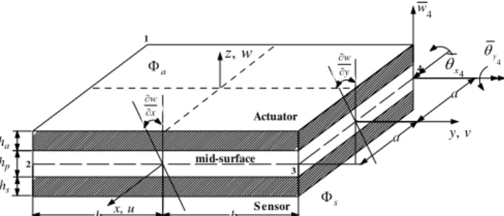
Figure 1. Coordinate system of a laminated finite element with integrated piezoelectric material.
Nomenclature
a = half length of the finite element in x direction, m
A = relative to surface area
b = half length of the finite element in y direction, m
C = elastic constant, N/m2
Cs = piezoelectric sensor capacitance, F
D = electric displacement vector, C/m2
e = piezoeletric stress coefficient, C/m2
E = Young’s modulus, N/m2
f = force, N
h = thickness, m
K = stiffness matrix
M = mass matrix
q = displacement field vector
qi = nodal displacement field, m
T = kinetic energy, J
u = displacement field in x direction, m
U = potential energy, J
v = displacement field in y direction, m V = volume, m3
w = displacement field in z direction, m
W = work, J
Greek Symbols
ε = strain field
σ = stress, N/m2 ν = Poisson ratio
θu = rotation about u-axis
ξ = dielectric tensor
ζ= nodal displacement vector Φ = electric potential, Volts
ω = frequency, rad/s
ρ = material density, kg/m3
Subscripts
a = refers to the actuator
b = relative to the body
p= relative to the plate structure
s = relative to the sensor
sa = relative to the sensed voltage in the actuator
x = relative to x direction
y= relative to y direction
qq = relative to the stiffness
qΦ = relative to the piezoelectric stiffness
ΦΦ = relative to the dielectric stiffness
Superscripts
e = relative to the element
S = relative to constant strain
T = matrix transpose
Finite Element Discretization
In the present formulation, the following assumptions (Reddy, 1999) are considered:
•the piezoelectric layers are perfectly bonded together; •the formulation is restricted to linear elastic material behavior (small displacement and strains);
•this formulation uses the Kirchhoff assumption (thin plate) in which the transverse normal remains straight after deformation and they also rotate such that they always remain perpendicular to the mid-surface.
Therefore, as shown in Fig. 1, the displacements field u, v, and
w can be expressed by the Kirchhoff hypotheses as (Reddy, 1999):
x w z u
∂ ∂ −
= , (1.1)
y w z v
∂ ∂ −
= , (1.2)
( )
x yw
w= , , (1.3)
where x and y are the in-plane axes located at the mid-surface of the plate, and z is along the plate thickness direction as seen Fig. 1. In addition, u and v are the displacements in the x and y-axes, respectively, whereas w is the transverse displacement (or also called deflection) along the z-axis.
Because the transverse shear deformation is neglected, the strain field can be written in terms of the displacements as:
{ }
{
}
T Txy y x
y x
w
y w
x w z
⎪⎭ ⎪ ⎬ ⎫ ⎪⎩
⎪ ⎨ ⎧
∂ ∂ ∂ ∂ ∂ ∂ ∂ − =
= 2
2 2 2 2
2
γ ε ε
ε . (2)
For isotropic material, the relation between plane stress (σ) and strain (ε) is given by:
{ }
σ =[ ]
D{ }
ε , (3)where
{ }
σ ={
σx σy τxy}
T and[ ]
D matrix is:[ ]
(
)
⎥⎥⎥ ⎦ ⎤ ⎢
⎢ ⎢ ⎣ ⎡
− −
=
2 1 0 0
0 1
0 1
1 2 ν
ν ν ν
p
E
D
,
(4)where ν is the Poisson ratio and Ep denotes the Young’s modulus of the plate.
Consider a four-node rectangular plate bending element based on classical plate theory (Bathe, 1982), where the element is shown in Fig. 1. Each node of the element possesses three degrees of freedom: a displacement w in the z direction; a rotation about x -axis (θx); and a rotation about y-axis (θy) as shown in the Fig. 1. The displacement function w is assumed to be:
(
)
3 12
3 11 3 10 2 9 2 8 3 7
2 6 5 2 4 3 2 1
,
i i
i i i i i i i i
i i i i i i i
i
y x c
y x c y c y x c y x c x c
y c y x c x c y c x c c y x w
+
+ +
+ + + +
+ + + + + + =
, (5)
⎪ ⎩ ⎪ ⎨ ⎧ = − = = = − = = − = − = = b y a x b y a x b y a x b y a x i 4 4 3 3 2 2 1 1 ; ; ; ; ; ; ; 4 1… (6)
The transversal displacement field (w) can be expressed by:
{ } { }
P cw= T , (7)
where the coefficient vector
{ }
c is represented by the relation given below:{ } {
}
Tc c c c c c
c = 1 2 3 4 5 … 12 , (8)
and
{ }
{
}
Txy y x y xy y x x y xy x y x
P = 1 2 2 3 2 2 3 3 3
.
(9)Vector
{ }
qi is defined as a nodal displacement field in the rectangular element:{ }
{
}
T y x y x y x y x i w w w w q 4 4 3 3 2 2 1 1 4 3 2 1 θ θ θ θ θ θ θ θ = , (10) where: i i y x i ww = , , (11.1)
i i
i x y
x y w , ∂ ∂ =
θ , (11.2)
i i
i x y
y x w , ∂ ∂ − =
θ . (11.3)
Combining Eqs. (5) and (10) with Eqs. (11.1), (11.2) and (11.3) at the four nodal points yields the following matrix expression:
{ }
qi =[ ]
X{ }
c , (12)where [X] is a 12 × 12 matrix given by Eq. (13).
[ ] ⎥ ⎥ ⎥ ⎥ ⎥ ⎥ ⎥ ⎥ ⎥ ⎥ ⎥ ⎥ ⎥ ⎥ ⎥ ⎥ ⎥ ⎥ ⎦ ⎤ ⎢ ⎢ ⎢ ⎢ ⎢ ⎢ ⎢ ⎢ ⎢ ⎢ ⎢ ⎢ ⎢ ⎢ ⎢ ⎢ ⎢ ⎢ ⎣ ⎡ − − − − − − − − − − − − − − − − − − − − − − − − − − − − = 3 4 4 2 4 2 4 4 4 2 4 4 4 2 4 4 3 4 2 4 4 4 2 4 4 4 3 4 4 4 3 4 3 4 2 4 4 4 2 4 3 4 2 4 4 4 2 4 4 4 3 3 3 2 3 2 3 3 3 2 3 3 3 2 3 3 3 3 2 3 3 3 2 3 3 3 3 3 3 3 3 3 3 3 2 3 3 3 2 3 3 3 2 3 3 3 2 3 3 3 3 2 2 2 2 2 2 2 2 2 2 2 2 2 2 2 3 2 2 2 2 2 2 2 2 2 3 2 2 2 3 2 3 2 2 2 2 2 2 2 3 2 2 2 2 2 2 2 2 2 3 1 1 2 1 2 1 1 1 2 1 1 1 2 1 1 3 1 2 1 1 1 2 1 1 1 3 1 1 1 3 1 3 1 2 1 1 1 2 1 3 1 2 1 1 1 2 1 1 1 3 0 2 3 0 2 0 1 0 3 3 2 0 2 0 1 0 0 1 3 0 2 3 0 2 0 1 0 3 3 2 0 2 0 1 0 0 1 3 0 2 3 0 2 0 1 0 3 3 2 0 2 0 1 0 0 1 3 0 2 3 0 2 0 1 0 3 3 2 0 2 0 1 0 0 1 y y x y y x x y x y x x y y x x y x y x y x y y x y x x y y x x y x y y x y y x x y x y x x y y x x y x y x y x y y x y x x y y x x y x y y x y y x x y x y x x y y x x y x y x y x y y x y x x y y x x y x y y x y y x x y x y x x y y x x y x y x y x y y x y x x y y x x y x X (13)
Therefore, the coefficient vector
{ }
c can be computed from Eq. (12), as:{ }
c =[ ]
X −1{ }
qi . (14)Substituting Eq. (14) into (7) yields:
[ ]
Nw{ }
qiw= , (15)
where
[ ]
Nw is the shape function matrix in the z direction given by:[ ]
N ={ }
PT[ ]
X −1w . (16)
Substituting Eq. (16) into (2) results in the following equation:
{ }
{ }
{ }
{ }
[ ]
{ }
iT T T T q X y x P y P x P z 1 2 2 2 2 2 2 − ⎪⎭ ⎪ ⎬ ⎫ ⎪⎩ ⎪ ⎨ ⎧ ∂ ∂ ∂ ∂ ∂ ∂ ∂ − =
ε (17)
Manipulating Eq. (17) it is possible to obtain:
{ }
ε =−z[ ][ ]
LK X −1{ }
qi , (18)in which
[ ]
⎥ ⎥ ⎥ ⎦ ⎤ ⎢ ⎢ ⎢ ⎣ ⎡ = 2 2 6 6 0 4 4 0 0 2 0 0 0 0 6 0 6 2 0 0 2 0 0 0 0 0 0 6 0 0 2 6 0 0 2 0 0 0 y x y x xy y x xy y xLK . (19)
The displacement field u, v, and w can be expressed by vector
{ }
q as:{ } {
}
Tv u w
q = . (20)
Substituting Eqs. (1.1), (1.2) and (1.3) into (20) yields:
{ }
Ty w z x w z w q ⎭ ⎬ ⎫ ⎩ ⎨ ⎧ ∂ ∂ − ∂ ∂ −
= . (21)
Substituting Eq. (15) into (21) gives the expression below:
{ }
[ ][ ] [ ]
{ }
iT
M X q
L H
q = −1 , (22)
where
[ ]
LM Tand [H] are given by:[ ]
T{ }
T{ }
T{ }
T TM y P x P P L ⎪⎭ ⎪ ⎬ ⎫ ⎪⎩ ⎪ ⎨ ⎧ ∂ ∂ ∂ ∂
= , (23.1)
[ ]
⎥ ⎥ ⎥ ⎦ ⎤ ⎢ ⎢ ⎢ ⎣ ⎡ − − = z z H 0 0 0 0 0 0 1 . (23.2)Fundamental Formulation of the Piezoelectric
Phenomena
In this work the following linear constitutive relations for piezoelectric materials are employed (Taylor et al., 1985):
{ }
σ =[ ]
CE{ }
ε −[ ]
e{ }
E , (24)where the superscript S means that the values are measured at constant strain and the superscript E means that the values are measured at constant electric field, {σ} is the stress tensor, {D} is the electric displacement vector, {ε} is the strain tensor, {E} is the electric field, [CE] is the elastic constants at constant electric field, [e] denotes the piezoelectric stress coefficients, and [ξS] is the dielectric tensor at constant mechanical strain.
The relation between [e] and [d], the piezoelectric strain coefficient, is:
[ ]
e =[ ][ ]
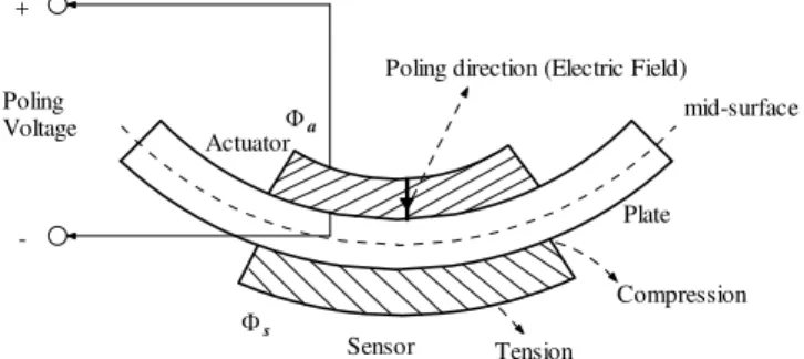
CE d . (26)The application of voltage to the element is analogous to the application of heat to a bimetallic strip. The voltage Φa across the bender element forces the bottom layer to expand, while the upper layer contracts, as depicted in Fig. 2.
Poling direction (Electric Field)
Φa
Compression
Tension
mid-surface
Sensor Actuator
Plate
Φs Poling
Voltage +
-Figure 2. Curvature of a plate produced by the expansion of one piezoelectric layer and contraction of the other.
The result of these physical changes is a strong curvature; this implies in a large deflection at the tip when the other end is clamped (see Fig. 2). The tip deflection may be much larger than the change in length of either ceramic layer. Due to the reciprocity effect, deformation of the sensor will produce a charge across the sensor electrode, which is collected through the sensor surface as an electric voltage Φs.
When only the poling direction is taken into account, the applied or sensed electric potential through the actuator or sensor element is given by the following equation (Lopes et al., 2000):
Φ ⎟ ⎟ ⎟ ⎟
⎠ ⎞
⎜ ⎜ ⎜ ⎜
⎝ ⎛
− = Φ
h h z p
z 2
,
(27)where h and Φ (see Fig. 2) are the thickness and the maximum electric potential at the external surface of the corresponding piezoelectric element (actuator and sensor), and z (za and zs) is defined over the intervals:
a p a p
h h z h
+ ≤ ≤
2
2
,
(28.1)s p s p
h h z h
− − ≥ ≥ −
2
2
.
(28.2)Now, assuming that the electric field (E) is constant through the actuator and sensor elements thickness, the gradient operators are:
h B dz d
E z z
Φ − = Φ − = Φ −
=
.
(29)Obtaining the Element Matrices
Hamilton’s principle is employed here to derive the finite element equations.
(
)
[
]
∫
2δ − + − +δ =1
0 t
t
m
e W W dt
W U
T , (30)
where t1 and t2 are two arbitrary instants, T is the kinetic energy, U
is the potential energy, We denotes the work done by electrical forces, and Wm is the work done by magnetic forces, which is negligible for piezoelectric materials. The total kinetic energy T and the potential energy U of the composite structure are described by the following relations:
{ } { }
∫
= V
T qdV
q
T ρ
2 1
, (31.1)
{ } { }
∫
= V
T dV
U ε σ
2 1
, (31.2)
where {q} is the differentiation of {q} with respect to t, {q} is given by Eq. (22) and dV is defined by:
s a
p dV dV
dV
dV= + + (32)
where the subscript p, a and s refer to the plate, actuator and sensor elements, respectively, and dVp, dVa, and dVs are given by:
∫ ∫ ∫
− − −= /2
2 /
p
p
h
h b
b a
a
p dxdydz
dV , (33.1)
∫
+∫ ∫
− −= p a
p
h h
h
b
b a
a
a dxdydz
dV
2 /
2 /
, (33.2)
∫
−− −∫ ∫
− −= /2
2 /
p
s p
h
h h
b
b a
a
s dxdydz
dV . (33.3)
The work done by electrical forces and magnetic forces is given by:
{ } { }
∫
= V
T
e E DdV
W
2 1
, (34.1)
{ } { }
{ } { }
∫
∫
+∫
− Φ=
A q
V A
A T b
T f dV q f dA dA
q
W δ δ δ σ
δ , (34.2)
where D is the electric displacement vector, fb is the body force, fA is the surface force, and σq is the surface electrical stress.
Substituting Eqs. (24) into Eq. (31.2) and substituting Eq. (25) into (34.1) yields, respectively:
{ }
[ ]
{ }
{ }
[ ]
{ }
∫
−∫
=
V V
T E
TC e EdV
U ε ε ε
2 1 2
1
{ }
[ ]
{ }
{ }
[ ]
{ }
∫
+∫
= V V S T T Te E e E EdV
W ε ξ
2 1 2
1
. (36)
Substituting Eqs. (31.1), (34.2), (35), and (36) into (30), results:
{ } { }
{ }
[ ]
{ }
{ }
[ ]
{ }
{ }
[ ]
{ }
{ }
[ ]
{ }
{ } { }
{ } { }
∫
∫
∫
∫
∫
∫
∫
∫
∫
= ⎪ ⎪ ⎪ ⎪ ⎪ ⎪ ⎭ ⎪⎪ ⎪ ⎪ ⎪ ⎪ ⎬ ⎫ ⎪ ⎪ ⎪ ⎪ ⎪ ⎪ ⎩ ⎪⎪ ⎪ ⎪ ⎪ ⎪ ⎨ ⎧ Φ − + + + + + + + + − 2 1 0 t t A q A A T V b T V S T V T V T T V V E T T dt dA dV f q dV f q dV E E dV e E dV E e c dV q q σ δ δ δ ξ δ ε δ δε ε δε δ ρ . (37)Substituting Eqs. (22), (18) and (29) into (37), yields:
{ }
[
[ ]
{ }
[ ]
{ }
[ ]
{ }
{ }
]
{ }
[
[ ]
{ }
[ ]
{ } { }
]
∫
= ⎪⎭ ⎪ ⎬ ⎫ ⎪⎩ ⎪ ⎨ ⎧ + Φ + Φ + − Φ + + ΦΦ Φ Φ 2 1 0 t t a e k e q e q k e qq k e qq T k dt Q K q K f K q K q M q δ δ , (38) where:[ ]
=∫
[ ] [ ][ ] [ ][ ] [ ]
− − V T M T M T eqq X L H H L X dV
M ρ 1 , (39.1)
[ ]
=[ ]
−∫
[ ] [ ][ ][ ]
− V K T K T eqq X z L D L X dV
K 2 1 , (39.2)
[ ] [ ]
[ ]
−∫
[ ] [ ]
Φ
Φ = =−
V z T T K T T e q e
q K X zL e B dV
K , (39.3)
[ ]
K B[ ]
BzdVV T T z e =−
∫
ΦΦ ξ , (39.4)
{ }
=∫
{ }
+∫
{ }
AA
V
b dV f dV
f
f
,
(39.5){ }
=∫
A q
a dA
Q σ . (39.6)
Allowing arbitrary variations of {qk} and {Φ}, two equilibrium equations written in generalized coordinates are now obtained for the k-th element:
{ }
[ ]{ }
[ ]{ }
{ }
0]
[Mqqe qk + Kqqe qk + KqeΦ Φ − f = , (40)
[ ]
KΦeq{ }
qk +[ ]
KΦΦe{ } { }
Φ + Qa =0, (41)where
[ ]
Ke is the extended element stiffness matrix and [Mqqe ] is the element mass matrix.Integrating the mechanical stiffness matrix [Kqqe ] in the z direction yields:
[ ] [ ] [ ][ ] [ ]
∑
∫
= − − = 3 1 1 ] [ i A K i T K T i eqq h X L D L dAX
K
,
(42)where hi is given by:
12 2 2
3 2
1 a a
p a h h h h
h ⎟⎟ +
⎠ ⎞ ⎜⎜ ⎝ ⎛ +
= , (43.1)
12
3
2 p
h
h = , (43.2)
12 2 2
3 2
3 s s
p s h h h h
h ⎟⎟ +
⎠ ⎞ ⎜⎜ ⎝ ⎛ +
= , (43.3)
and [Di] or [Da], [Dp], and [Ds], for i = 1,2,3, are calculated by Eq. (4) for the piezoelectric and plate material properties, respectively, and dA is equal to dxdy.
The element mass matrix is integrated in the z direction resulting:
[ ] [ ] [ ][ ] [ ]
∑
∫
= − − = 3 1 1 ] [ i A M i T M T i eqq X L H L dA X
M ρ , (44)
where ρ1=ρa, ρ2=ρp, ρ3=ρs, and
[ ]
Hi (for i = 1,2,3) are:[ ] [ ]
⎥ ⎥ ⎥ ⎦ ⎤ ⎢ ⎢ ⎢ ⎣ ⎡ = = 1 1 0 0 0 0 0 0 h h h H H a ai , (45.1)
[ ]
[ ]
⎥ ⎥ ⎥ ⎦ ⎤ ⎢ ⎢ ⎢ ⎣ ⎡ = = 2 2 2 0 0 0 0 0 0 h h h H H pp
,
(45.2)[ ] [ ]
⎥ ⎥ ⎥ ⎦ ⎤ ⎢ ⎢ ⎢ ⎣ ⎡ = = 3 3 3 0 0 0 0 0 0 h h h H H ss
.
(45.3)The electrical-mechanical coupling stiffness matrix [KqeΦ] and dielectric stiffness matrix [KΦΦe ] are integrated in the z direction with respect to the thickness of each piezoelectric layer (where dV =
dVa and dV = dVs), yielding:
[ ]
(
)
[ ] [ ] [ ]
−∫
Φ =− +
A z T a T K T a a p a e
q h h h X L e BdA
K 2 2 1 , (46.1)
[ ]
[ ]
a S a a e h abKΦΦ =−4 ξ , (46.2)
[ ]
(
)
[ ] [ ] [ ]
−∫
Φ = +
A z T s T K T s s p s e
q h h h X L e BdA
K 2
2 1
[ ]
[ ]
s S s s
e
h ab
KΦΦ =−4 ξ . (46.4)
The Eqs. (42), (44), (46.1), and (46.3) are integrated numerically by using the Gauss-quadrature integration method (Bathe, 1982):
[ ]
[ ] [ ][ ]
[ ]
∑
∑∑
=
− −
=
3 1
1
] [
i
K i T K T
i e
qq h X L D L WW X
K
η ξ
ξ η , (47.1)
[ ]
[ ] [ ][ ]
[ ]
∑
∑∑
=
− −
=
3
1
1
] [
i
M i T M T
i e
qq X L H L WW X
M
η ξ
ξ η
ρ , (47.2)
[ ]
(
)
[ ]
−∑∑
[ ] [ ]
Φ =− +
η ξ
ξ η z
T a T K T
a a p a e
q h h h X L e W W B
K 2
2
1 , (47.3)
[ ]
(
)
[ ]
−∑∑
[ ] [ ]
Φ = +
η ξ
ξ η z
T s T K T
s s p s e
q h h h X L e W W B
K 2
2
1 , (47.4)
where (ξ, η) are the Gaussian integration point coordinates and Wξ
and Wη are the associated weight factors.
Obtaining the Global Matrices
Each of these element matrices can be assembled into global matrices. The assemblage process to obtain the global matrices is written as:
[ ]
∑
[ ]
[ ]
[ ]
= =
N
k
k e qq T
k M T
T M
1
, (48)
[ ]
∑
[ ]
[ ]
[ ]
= =
N
k
k e qq T k
qq T K T
K
1
, (49)
where N is the number of finite elements and
[ ]
Tk is the distribution matrix defined by:( )
( )
( )
⎩ ⎨ ⎧
= ≠ =
i m j if
i m j if j i T
k k k
1 0
, ,
for i =1, 2, …, 12, and j = 1, 2, …,ndof (50) where ndof is the number of degrees of freedom of the entire structure, and mk denotes the index vector containing the degrees of freedom (3 dof) of the n-th node (1, 2, 3 or 4 – see Fig. 1) in the k-th finite element given by:
{
k k k}
k n n n
m = 3 −2 3 −1 3
,
(51)Considering that na actuators and ns sensors are distributed in the plate, Eqs. (40) and (41) can be written in the global form:
{ }
[ ]{ }
[ ]
[ ]{ } { }
0] [
1
= − Φ +
+ Φ
=
∑
T K FK
M q i
n
k T i k qq
i e ζ
ζ , (52)
[ ]
[ ]
{ }
[
]
{ }
(
)
∑
= Φ ζ + ΦΦ Φ + =
i e n
k
a i i
k i
q T K Q
K
1
0 , (53)
where
[ ]
Tk i is the distribution matrix (Eq. 50) which shows the position of the k-th element in the plate structure by using zero-one inputs, where the zero input means that no piezoelectric actuator/sensor is present, and one input means that there is an actuator/sensor in that particular element position, nei is the numberof finite elements of the i-th piezoelectric actuator/sensor, and
{ }
ζ is the nodal displacement vector of the global structure.In the piezoelectric sensor there is no voltage applied to the corresponding element (Qa = 0), so that the electrical potential generated (sensor equation) is calculated by using Eq. (53), yielding:
{ }
∑
[
]
[ ]
[ ]
{ }
=
Φ − ΦΦ − = Φ
i e
n
k
i k si q si
s K K T
1
1 ζ for i = 1, 2, …, n
s (54)
The total voltage
{ }
Φ is composed by the voltage{ }
Φs that is sensed by the sensor, the voltage{ }
Φsa that is sensed by the actuator (see Eq. 54), and by the applied voltage{ }
Φa . Then,{ }
Φ can be expressed by the following equation:{ } { } { } { }
Φ = Φs + Φsa + Φa . (55)The global dynamic equation can be formed by substituting Eq. (54) into Eq. (55) and then into Eq. (52). Thus, moving the forces due to actuator together with the mechanical forces to the right hand side of the resulting equation, yields:
[ ]
M{ }
ζ +[Kqq* ]{ } { } { }
ζ = F + Fel j, (56)where ][K*qq , and
{ }
Fel (electrical force) are given by, respectively:[ ]
qq[ ]
elqq K K
K ]= −
[ * , (57)
and
{ }
[ ]
[ ]
q aj ajn
k T
j k j
el T K
F
j e
Φ −
= Φ
=
∑
1
, for j = 1, 2, …, na (58)
where
[ ]
Kel is the electric stiffness written as:[ ]
[ ]
[ ]
[
]
[ ]
[ ]
[ ]
[ ]
[
]
[ ]
[ ]
∑∑
∑∑
= =
Φ − ΦΦ Φ
= =
Φ − ΦΦ
Φ +
=
a ej
s ei
n
j n
k
j k aj q aj aj q T
j k n
i n
k
i k si q si si q T i k el
T K K K T
T K K K T K
1 1
1 1 1
1
. (59)
The system static equation is written by using Eq. (33) as follows:
{ }
ζ =[K*qq]−1(
{ } { }
F + Fel)
. (60)Closed Form Solutions for Rectangular Plates
(
x yt)
f w h w
D∇4 +ρp p = , ,
,
(62)where
( )
23
1 12 −ν = Ehp
D is the flexural rigidity of the plate, and
4 4
2 2
4
4 4 4
2
y w y x
w x
w
∂ ∂ + ∂ ∂
∂ + ∂ ∂ =
∇ is known as the biharmonic
operator.
The response of the plate can be written assuming that the solution is of the form:
(
)
∑∑
∞( ) ( )
= ∞
= =
1 1
, ,
,
k l
kl
kl x y t
t y x
w φ η , (63)
where φ(x,y) is a function of the spatial coordinates given by (Dimitriadis, 1991):
( )
( ) ( )
b l a k y sin x sin y
x k l k l
kl
π γ π γ γ γ
φ , = ; = ; = , (64)
ηkl(t) is a function of time, Lx and Lyare the plate length and width, respectively, and m = n = 1,2,3, ...
According to Dimitriadis (1991), assuming that the piezoelectric elements are perfectly bonded to the plate surface, which implies that strain continuity is satisfied at the interface, the external loading of the plate, represented by the actuator induced moments, can be written as:
(
)
⎟⎟⎠ ⎞ ⎜
⎜ ⎝ ⎛
∂ ∂ + ∂ ∂ Λ
= 0 22 22
, ,
y R x
R C t y x
f , (65)
where:
(
)
20
1 1 1 1 12
1
p a p p a
p h
P P E
C
ν ν ν ν
+ − + − + −
= , (66.1)
(
)
3 2 3 2 2
8 6 6 1 1
a a p p
a p a p
a p
p a
h h h h
h h h h E
E P
+ +
+ −
− − − =
ν ν
, (66.2)
a a
h d Φ
=
Λ , (66.3)
( )
x,y[
H(
x xa1) (
H x xa2)
]
[
H(
y ya1) (
H y ya2)
]
R = − − − − − − . (66.4)
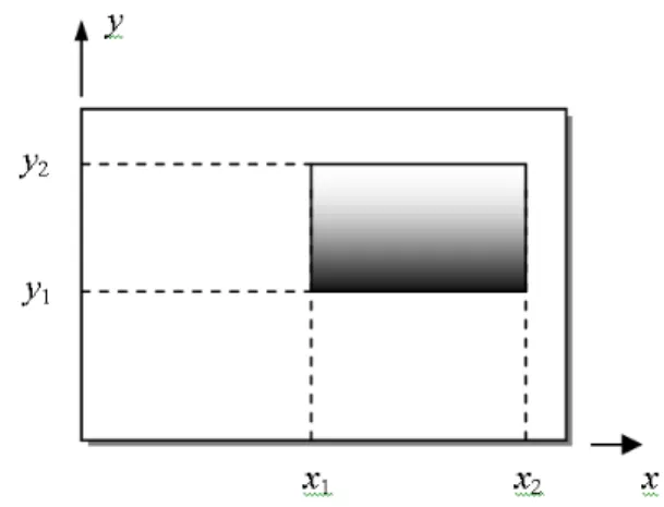
Λis the induced strain, d is given by Eq. (26), Φa is the applied voltage, R(x,y) is the generalized location function expressed as a function of the Heaviside function (Southas-Little and Inman, 1999), and
1
a
x ,
2
a
x and
1
a
y ,
2
a
y are the boundaries of the piezoelectric actuator (see Fig. 3).
Figure 3. Plate and piezoelectric material coordinate system.
Fuller et al. (1996) have derived an expression for the charge generated by a two-dimensional distributed sensor, which is given by:
( )
(
)
∫ ∫
⎟⎟⎠ ⎞ ⎜
⎜ ⎝ ⎛
∂ ∂ + ∂ ∂ +
= 2
1 2 1
2 2
32 2 2
31
2
1 s
s s
s
y
y x
x s s
s p
s dxdy
y w e x
w e h
h t
Q , (67)
where es is the piezoelectric material stress constant and xs1, xs2
and
1
s
y ,
2
s
y are the boundaries of the piezoelectric sensor. The electrical voltage generated by the sensor can be obtained through the following relation:
( )
( )
s s s
C t Q t =
Φ , (68)
where Cs is the sensor capacitance.
Considering that ns sensors are distributed on the plate, and substituting Eq. (63) into (67) and then into (68), yields (assuming es = es31 = es32) (Fuller et al, 1996):
(
h h)
( )
tC e
kl
k l
s s
p s s
s i i
i
i
∑∑
η∞
= ∞
= Γ +
= Φ
1 1
2 , for i = 1, 2, …, ns (69)
where
i
s
Γ is given by:
(
cos i2 cos i1)(
cos i2 cos i1)
i k s k s l s l s
k l l k
s γ γ x γ x γ y γ y
γ γ γ
− −
⎟⎟ ⎠ ⎞ ⎜⎜
⎝ ⎛
+ =
Γ . (70)
Considering also that na actuators are distributed on the plate, the dynamical equation of the system is obtained by substituting Eqs. (65) and (63) into (62), yielding:
( )
( )
∑
( )
=
Φ Γ =
+
a
j j j j kl
n
j
a a a
j
p p y x kl n
kl t
h d C h L L t t
1 0
2 4
ρ η
ω
η , (71)
where:
(
cos 1 cos 2)(
cos 2 cos 1)
2 2
j j
j j
j l a l a k a k a
l k
l k
a γ γ γ y γ y γ x γ x
γ γ
− −
+ =
Γ , (72)
(
2 2)
l k p p n
h D
kl ρ γ γ
ω = + . (73)
The static solution for the application of a constant electric voltage to the actuators can be obtained by substituting ηkl (calculated from Eq. 71) into Eq. (63), yielding:
( )
∑∑
∞( )
∑
( )
= ∞
= =
Φ Γ =
1 1 1
0 2
, 4
,
k l
n
j
a a a
j
n kl
p p y x
a
j j j j
kl
t h
d C y x h
L L y x w
ω φ
ρ . (74)
Numerical Examples (Model Validation)
In order to verify the accuracy of the presented finite element formulation2, the numerical results are compared with the close form solutions and with those from software ANSYS®.
Static Displacement Distribution
The first validation case is the comparison between the static displacement distribution obtained from the numerical techniques presented.
In the upcoming validations a rectangular plate and piezoelectric material with the following characteristics are used (see Table 1):
Table 1. Material and geometrical properties of plate and piezoelectric.
Piezoelectric
Properties Sensor Actuator Plate
E (Young’s modulus) 2 69 207
ρ(Density) 1780 7700 7870
ν (Poisson) 0.3 0.3 0.29
h (Thickness) 0.205×10⁻³ 0.254×10⁻³ 1×10⁻³
ξS
(Piezo dielectric) 1.06×10⁻¹⁰ 1.6×10⁻⁸ ----
e (Piezoelectric strain) 0.046 -12.5 ----
C (Capacitance) 5.2×10⁻⁹ 6.3×10⁻⁷ ----
Geometry (Lx× Ly) 0.1×0.1 0.1×0.1 0.6×0.4
The influence of the piezoelectric patches on the static behavior of the structure is investigated.
The configuration, illustrated in Fig. 4, shows the corresponding layout of the piezoelectric actuators and sensors symmetrically bonded to the plate surfaces.
x L Y
X
y
L
1
2 3
Figure 4. Piezoelectric actuators and sensors test configuration.
2 The structure was modeled by a 24×16 finite element mesh (N =384).
The placements of the piezoelectric elements are shown in Table 2.
Table 2. Piezoelectric element positions on the plate structure.
Material
Position (m) 1 2 3
x1 0.25 0.15 0.35
y1 0.05 0.25 0.25
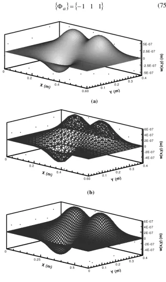
Figure 5 shows the total plate displacement amplitude calculated by using Eq. (74) – closed form solution, Eq. (60) – FEM, and software3 ANSYS®,when a static input voltage (Φa) is applied to actuators (1, 2 and 3) for the following magnitude:
{ } {
Φa = −1 1 1}
(75)-5E-07 -2.5E-07 0 2.5E-07 5E-07
w
(x,
y)
(m
)
0
0.2
0.4
0.6
X (m)
0
0.1 0.2 0.3
0.4
Y (m)
(a)
-4E-07 -2E-07 0 2E-07 4E-07 6E-07
w(
x
,y
)
(m
)
0
0.2
0.4
0.6
X (m)
0
0.1 0.2
0.3 0.4
Y (m)
(b)
-4E-07 -2E-07 0 2E-07 4E-07 6E-07
w(
x
,y
)
(m
)
0
0.25
0.5
X (m)
0 0.1 0.2
0.3 0.4
Y (m)
(c)
Figure 5. Static displacement distribution obtained by using the closed form solution (a), the finite element technique (b), and software ANSYS® (c).
As can be seen from Fig. 5, both approaches give close results for the static displacement distribution.
3
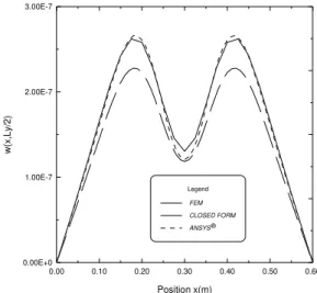
The static displacement distribution is calculated by using numerical techniques for two particular sections of the plate (y =
Ly/2 and x = Lx/2), as illustrated in Figs. 6 and 7, respectively.
0.00 0.10 0.20 0.30 0.40 0.50 0.60
Position x(m)
0.00E+0 1.00E-7 2.00E-7 3.00E-7
w(x
,Ly/
2
)
Legend
FEM CLOSED FORM ANSYS®
Figure 6. Comparison of the static displacement distribution (section y =
Ly/2) for the numerical techniques presented.
0.00 0.10 0.20 0.30 0.40
Position y (m)
-6.00E-7 -3.00E-7 0.00E+0 3.00E-7 6.00E-7
w
(L
x
/2
,y
) (m
)
Legend
FEM CLOSED FORM ANSYS®
Figure 7. Comparison of the static displacement distribution (section x =
Lx/2) for the numerical techniques presented.
The electric potentials generated by the piezoelectric sensors are then computed by using Eq. (69) where ηkl is given by:
( )
∑∑ ∑
∞= ∞
= =
Φ Γ =
1 1 1
0 2
1 4
k l
n
j
a a a
j
n p
p y x kl
a
j j j j
kl
t h
d C h
L
L ρ ω
η . (76)
The obtained results for each technique used can be seen in Table 3.
Table 3. Electric potentials generated by the piezoelectric sensors.
Electric Potential (Volts) Sensor FEM CLOSED FORM ANSYS®
1 +0.0162178 +0.0139268 +0.0116576
2 -0.0162150 -0.0139280 -0.0115743
3 -0.0162150 -0.0139280 -0.0115743
As can be observed the results presented again satisfactory agreement.
Dynamic Displacement Distribution
Now the closed form solution for thin rectangular plates for two-dimensional piezoelectric elements with simply supported boundary conditions, the present finite element technique, and the software ANSYS® are used to calculate the total displacement distribution in
z direction for the structure for various excitation frequencies, using the piezoelectric actuators/sensors configuration as shown in Fig. 4. The analysis of the dynamic response of the plate due to the excitation caused by a sinusoidal voltage applied to the actuator layer with no mechanical loading at different time instants is shown.
The value of the applied voltage amplitude (Φ) was 1.0 Volt and the excitation frequency (ω) was 185 rad/s for the actuator 1, 310 rad/s for the actuator 2, and 440 rad/s for the actuator 3. The excitation frequencies are chosen between two natural frequencies of modes (k,l) (see Eq. 73): (1, 1) and (2, 1) for the first excitation frequency, (2,1) and (1,2) for the second, and (1,2) and (3,1) for the third excitation frequency.
The results for the displacement distribution in z direction, by using the closed form solution (see Eq. 63, where ηkl is obtained by Eq. 71), are compared with those obtained from the present finite element model (Eq. 56) and software ANSYS® (time increment: 0.1
ms).
Figures 8, 9, and 10 show the transversal displacement distribution w(x,y,t) for three different time instants: 0.005, 0.01, and 0.02 seconds, respectively.
-4E-07 -2E-07 0 2E-07 4E-07
w
(x,
y)
(m
)
0
0.2
0.4
0.6
X (m)
0 0.1 0.2 0.3 0.4
Y (m)
(a)
-4E-07 -2E-07 0 2E-07 4E-07
w
(x,
y)
(m
)
0
0.2 0.4
0.6
X (m)
0 0.1 0.2 0.3 0.4
Y (m)
(b)
-4E-07 -2E-07 0 2E-07 4E-07
w(
x
,y
)
(m
)
0
0.25
0.5
X (m)
0 0.1 0.2 0.3 0.4
Y (m)
(c)
Figure 9. Dynamic displacement distribution (at 0.01 s) obtained by using closed form solution (a), the present finite element technique (b), and software ANSYS® (c).
-6E-07 -4E-07 -2E-07 0 2E-07 4E-07
w
(x,
y)
(m
)
0
0.2
0.4
0.6
X (m)
0 0.1 0.2 0.3 0.4
Y (m)
(a)
Figure 10. Dynamic displacement distribution (at 0.02 s) obtained by using closed form solution (a), the present finite element technique (b), and software ANSYS® (c).
-6E-07 -4E-07 -2E-07 0 2E-07 4E-07
w(
x
,y
)
(m
)
0
0.2 0.4
0.6
X (m)
0 0.1 0.2 0.3 0.4
Y (m)
(b)
-6E-07 -4E-07 -2E-07 0 2E-07 4E-07
w(
x
,y
)
(m
)
0
0.25
0.5
X (m)
0 0.1 0.2 0.3 0.4
Y (m)
(c)
Figure 10. (Continued).
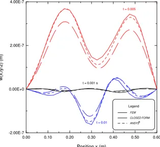
The dynamic displacement distributions in two particular sections of the plate (y = Ly/2 and x = Lx/2) are illustrated in Figs. 11 and 12, respectively.
0.00 0.10 0.20 0.30 0.40 0.50 0.60
Position x (m) -2.00E-7
0.00E+0 2.00E-7 4.00E-7
w(x,ly
/2) (m)
® t = 0.001 s
t = 0.005
t = 0.01
Legend
FEM CLOSED FORM ANSYS
Figure 11. Comparison of the dynamic displacement distribution (section
0.00 0.10 0.20 0.30 0.40
Position y (m) -1.20E-6
-8.00E-7 -4.00E-7 0.00E+0 4.00E-7 8.00E-7
w(lx/2
,y) (m)
Legend
FEM CLOSED FORM ANSYS®
t = 0.005 s
t = 0.001 s
t = 0.01 s
Figure 12. Comparison of the dynamic displacement distribution (section
x = Lx/2) at time instants: 0.005 s, 0.01 s, and 0.02 s.
Finally, the electric potentials generated by the sensors in the time interval from 0 to 0.01 seconds are illustrated in Fig. 13.
0.00E+0 2.00E-3 4.00E-3 6.00E-3 8.00E-3 1.00E-2
Time (s)
-0.02 -0.01 0.00 0.01 0.02
Vo
lt
ag
e (
V
o
lts
)
Legend FEM CLOSED FORM ANSYS®
Sensor 1
Sensor 2
Sensor 3
Figure 13. Comparison of the electric potential responses of each sensor.
The results above show that the present modeling technique is also effective for the dynamic response of the plate due to an excitation caused by the actuator layer in comparison with the results from the closed form solutions and the software ANSYS®. Small differences found for the transversal displacement values are due to the consideration of the 3D solid elements used in the ANSYS® model formulation.
It is important to mention that, as closed form solutions do not include mass and stiffness effects from the piezoelectric, significant differences with respect to the other techniques are found, according to Figs. 6, 7, 11 and 12.
Conclusions
A finite element formulation based on Kirchhoff’s plate model has been developed for the analysis of smart composite structures with piezoelectric materials.
All important steps were presented in detail, in such a way that the modeling technique used can be easily understood. Besides, various computational tests were performed (static and dynamic ones) demonstrating the efficiency of the methodology used.
Results were presented for a simply supported rectangular thin plate excited and sensed by various rectangular actuators and sensors bonded symmetrically to both sides of the plate. The results for the static and dynamic analysis obtained by the present finite element technique show good agreement with those from the exact solutions and software ANSYS®. The present solutions are useful for understanding the electromechanical coupling in intelligent structures under dynamic conditions. Besides, the present methodology is useful for the design of vibration control devices.
Acknowledgement
The first author is thankful to Capes Foundation (Brazil) for his doctorate scholarship. The third author is thankful to CNPq (Proc. Nº 470082/03-8).
References
Bathe, K-J., 1982, “Finite Element Procedures in Engineering Analysis”, Prentice-Hall.
Charette, F.; Berry, A. and Guigou, C., “Dynamic Effects of Piezoelectric Actuators on the Vibrational Response of a Plate”, Journal of Intelligent Material Systems and Structures, Vol. 8, pp. 513-524.
Chen, Chang-qing; Wang, Xiao-ming and Shen, Ya-peng, 1996, “Finite Element Approach of Vibration Control Using Self-Sensing Piezoelectric Actuators”, Computers & Structures, Vol. 60, No. 3, pp. 505-512.
Chou, Jyh-Horng; Chen, Shinn-Horng; Chang, Min-Yung and Pan, An-Jia, 1997, “Active Robust Vibration Control of Flexible Composite Beams with Parameter Perturbations”, International Journal of Mechanical Science, Vol. 39, No. 7, pp. 751-760.
Crawley, E. F. and de Luis, J., 1987, “Use of Piezoelectric Actuators as Elements of Intelligent Structures”, AIAA Journal, Vol. 25, No. 10, pp. 1373-1385.
Dimitriadis, E. K.; Fuller, C. R. and Rogers, C. A., 1991, “Piezoelectric Actuators for Distributed Vibration Excitation of Thin Plates”, Transactions of the ASME, Vol. 113, pp. 100-107.
Fuller, C. R., Elliott, S. J. and Nelson, P. A., 1996, “Active Control of Vibration”, Academic Press Ltd, San Diego, CA, p332.
Hagood, N. W. and von Flotow, A., 1991, “Damping of Structural Vibrations with Piezoelectric Materials and Passive Electrical Networks”, Journal of Sound and Vibration, Vol. 146, No. 2, pp. 243-268.
Hansen, S, 1998, “Analysis of a Plate with a Localized Piezoelectric Patch”, Conference on Decision & Control, Tampa, Flórida, pp. 2952-2957.
Lam, K. Y. and Ng, T. Y., “Active Control of Composite Plates with Integrated Piezoelectric Sensors and Actuators under Various Dynamic Loading Conditions”, Journal of Smart Materials and Structures, Vol. 8, pp. 223-237.
Ledda, A; Hornsby, J. H.; Riggs, J.; Blanas, P.; Shuford, R. J. and Das-Gupta, D. K., 1999, “Finite Element Modeling of Embedded Piezoelectric Sensors”, 10th International Symposium on Electrets, pp. 651-654.
Lima Jr, J. J., 1999, ''Modelagem de Sensores e Atuadores Piezelétricos com Aplicações em Controle Ativo de Estruturas'', Tese de Doutorado, Universidade Estadual de Campinas, Campinas-SP, p209.
Lin, Chien-Chang and Huang, Huang-Nan, 1999, “Vibration Control of Beam-Plates with Bonded Piezoelectric Sensors and Actuators”, Computers & Structures, No. 73, pp. 239-248.
Lopes, V. Jr.; Pereira, J. A. and Inman, D. J., 2000, “Structural FRF Acquisition Via Electric Impedance Measurement Applied to Damage Location”, XVII IMAC, San Antonio, EUA.
Reddy J. N., 1999, “Theory and Analysis of Elastic Plates”, Taylor and Francis.
Reddy, J. N., 1999, “On Laminated Composite Plates with Integrated Sensors and Actuators”, Engineering Structures, Vol. 21, pp. 568-593.
Soutas-Little, R. W. and Inmam, D. J., 1999, “Engineering Mechanics”, Statics, Prentice-Hall.
Tzou, H. S. and Tseng, C. I., 1990, “Distributed Piezoelectric Sensor/Actuator Design for Dynamic Measurement/Control of Distributed Parameter Systems: A Piezoelectric Finite Element Approach”, Journal of Sound and Vibration, Vol. 1, No. 138, pp. 1734.
Yang, S. M. and Lee, G. S., 1997, “Vibration Control of Smart Structures by Using Neural Networks”, Trans. of the ASME, Journal of Dynamic Systems, Measurement, and Control, Vol. 119, pp. 3439.
Appendix
In the software ANSYS®, the elastic (CE), piezoelectric (e), and dielectric (ξ) matrices for the actuator (a) and sensor (s) materials are defined below (see Table 1).
Actuator
[ ]
CEa=Ea,[ ]
⎥ ⎥ ⎥ ⎥ ⎥ ⎥ ⎥ ⎥
⎦ ⎤
⎢ ⎢ ⎢ ⎢ ⎢ ⎢ ⎢ ⎢
⎣ ⎡
− −
=
0 0 0
0 0 0
0 0 0
0 0 0
351 . 12 0 0
351 . 12 0 0
a
e ,
[ ]
⎥ ⎥ ⎥ ⎥
⎦ ⎤
⎢ ⎢ ⎢ ⎢
⎣ ⎡
× ×
× =
− −
−
8 8
8
10 6 . 1 0 0
0 10
6 . 1 0
0 0
10 6 . 1 a
ξ .
Sensor
[ ]
CEs=Es,[ ]
⎥ ⎥ ⎥ ⎥ ⎥ ⎥ ⎥ ⎥
⎦ ⎤
⎢ ⎢ ⎢ ⎢ ⎢ ⎢ ⎢ ⎢
⎣ ⎡
=
0 0 0
0 0 0
0 0 0
0 0 0
046 . 0 0 0
046 . 0 0 0
s
e ,
[ ]
⎥ ⎥ ⎥ ⎥
⎦ ⎤
⎢ ⎢ ⎢ ⎢
⎣ ⎡
× ×
× =
− −
−
10 10
10
10 06 . 1 0 0
0 10
06 . 1 0
0 0
10 06 . 1 s
ξ