Abs tract
Static analysis of skew composite shells is presented by develop-ing a C0 finite element (FE) model based on higher order shear
deformation theory (HSDT). In this theory the transverse shear stresses are taken as zero at the shell top and bottom. A realistic parabolic variation of transverse shear strains through the shell thickness is assumed and the use of shear correction factor is avoided. Sander’s approximations are considered to include the effect of three curvature terms in the strain components of com-posite shells. The C0 finite element formulation has been done
quite efficiently to overcome the problem of C1 continuity
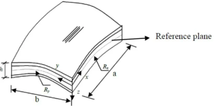
associ-ated with the HSDT. The isoparametric FE used in the present model consists of nine nodes with seven nodal unknowns per node. Since there is no result available in the literature on the problem of skew composite shell based on HSDT, present results are validated with few results available on composite plates/shells. Many new results are presented on the static re-sponse of laminated composite skew shells considering different geometry, boundary conditions, ply orientation, loadings and skew angles. Shell forms considered in this study include spheri-cal, conispheri-cal, cylindrical and hypar shells.
Key words
skew shell, composite, higher order shear deformation theory, cylindrical, hypar, finite element method
Analysis of laminated composite skew shells using
higher order shear deformation theory
1 INTRODUCTION
Laminated composite shell structures are widely used in civil, mechanical, aerospace and other en-gineering applications. Laminated composites materials are becoming popular because of their high strength to weight and strength to stiffness ratios. The most important feature for the analysis of composite structures is that the material (composite) is weak in shear compared to extensional ri-gidity. Due to this reason transverse shear deformation of the composite shell has to be modeled very efficiently.
A j ay Ku mar*, A n up am
C ha krab arti an d Mru na l Ke tkar
Department of Civil Engineering, Indian Insti-tute of Technology, Roorkee-247 667, India Phone: +91(1332)285844,
Fax.: +91(1332)275568
Received 14Jun 2012 In revised form 09 Oct 2012
N om enclature
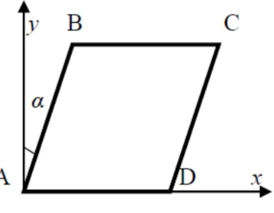
a = Length of the mappedshell panel parallel to x-axis in plan
α = Angle between skewed edge of mapped shell panel with respect to y-axis measured in plan
b = Width of the mapped shell panel parallel to y-axis in plan
h = Total height of the shell panel
N x N = FE mesh divison denoted as (Number of divisions in X-direction) x (Number of divisions
in Y-direction).
L = Total number of layers in a lamination scheme
Classical theories originally developed for thin elastic shells are based on the Love- Kirchhoff as-sumptions. These theories neglect the effect of transverse shear deformations. However, application of such theories to laminated composite shells where shear deformation is very significant, may lead to errors in calculating deflections, stresses and frequencies.
In subsequent development of shell theories transverse shear deformation was included in a manner where the shear strain is uniform throughout the thickness of the shell. These theories are known as first order shear deformation theory (FSDT). In this theory a shear correction factors are required for the analysis and these factors should be calculated based on the orientations of different layers in different directions.
The effects of transverse shear and normal stresses in shells were considered by Hildebrand, Reissner and Thomas [18], Lure [25], and Reissner [35]. The effect of transverse shear deformation and transverse isotropy, as well as thermal expansion through the thickness of cylindrical shells were considered by Gulati and Essenberg [16], Zukas and Vinson [43], Dong et al. [12, 13], Hsu and Wang [19], and Whitney and Sun [37, 38]. The higher-order shell theories presented in [37, 38] are based on a displacement field in which the displacements in the surface of the shell are expanded as linear functions of the thickness coordinate and the transverse displacement is expanded as a quad-ratic function of the thickness coordinate. These higher-order shell theories are cumbersome and computationally more demanding, because, with each additional power of the thickness co-ordinates, an additional dependent unknown is introduced into the theory.
Reddy and Liu [33] presented a simple higher-order shear deformation theory (HSDT) for the analysis of laminated shells. It contains the same dependent unknowns as in the first-order shear deformation theory (FSDT) in which the displacements of the middle surface are expanded as linear functions of the thickness coordinate and the transverse deflection is assumed to be constant through the thickness. The theory is based on a displacement field in which the displacements of the middle surface are expanded as cubic functions of the thickness coordinate and the transverse displacement is assumed to be constant through the thickness. The additional dependent unknowns introduced with the quadratic and cubic powers of the thickness coordinate are evaluated in terms of the derivatives of the transverse displacement and the rotations of the normals at the middle surface. This displacement field leads to the parabolic distribution of the transverse shear stresses (and zero transverse normal strain) and therefore no shear correction factors are used. Huang [20] presented modified Reddy’s theory and further improved the accuracy. Xiao-ping [39] presented a shell theory based on Love’s first-order geometric approximation and Donnell’s simplification for shallow shells. The theory improves the in-plane displacement (u, v) distribution through thickness by ensuring the continuity of interlaminar transverse shear stresses and zero transverse shear strains on the surface. The theory contains then same dependent unknown and the same order of governing equations as in the first-order shear deformation theory. Without the need for shear correction fac-tors, the theory predicts more accurate responses than first-order theory and some higher-order theories, and the solutions are very close to the elasticity solutions. However, these theories [33, 39] demand C1 continuity of transverse displacements during finite element implementations.
developed an improved higher-order theory for laminated composite plates. This theory satisfies the stress continuity across each layer interface and also includes the influence of different materials and ply-up patterns on the displacement field. Liew and Lim [24] proposed a higher-order theory by considering the Lame´ parameter (1+z/Rx) and (1+z/Ry) for the transverse strains, which were neglected by Reddy and Liu [33]. This theory accounts for cubic distribution (non-even terms) of the transverse shear strains through the shell thickness in contrast with the parabolic shear distri-bution (even-terms) of Reddy and Liu [33]. Kant and Khare [21] presented a higher-order facet quadrilateral composite shell element. Bhimaraddi [4], Mallikarjuna and Kant [26], Cho et al. [8] are among the others to develop higher-order shear deformable shell theory. It is observed that except for the theory of Yang [41], remaining higher-order theories do not account for twist curvature (1/Rxy), which is essential while analyzing shell forms like hypar and conoid shells.
Analyses of composite shell panels were carried out by many researchers [1, 4, 6, 7, 9, 14, 15, 22, 24, 27, 29, 30, 33 and 36] in the past few decades mainly based on FSDT.
However, application of higher-order theory for studying the behavior of laminated composite shells with the combination of all three radii of curvature is very limited in literature. Pradyumna and Bandyopadhyay [31] studied the behavior of laminated composite shells based on a higher-order shear deformation theory (HSDT) developed by Kant and Khare [21]. They also [21] also extended the theory to the shells to include all three radii of curvature. However, this theory [21] contains some nodal unknowns which are not having any physical significance and therefore, incorporation of appropriate boundary conditions becomes a problem.
It is also observed that there is no literature available on the analysis of composite skew shell us-ing HSDT while very few publications are available on the problem usus-ing FSDT [17] for isotropic materials only.
In view of the above, a new finite element model has been developed in the present study for static analysis of composite skew shell panels using a simple higher order shear deformation theory [33]. The problem of C1 continuity associated with theory has been overcome in this model and an existing C0 isoparametric finite element has been utilized for this purpose. The element contains nine nodes with seven nodal unknowns at each node. The analysis has been performed considering shallow shell assumptions. The effect of all the three radii of curvature is also included in the for-mulation. The present finite element model based on HSDT is applied to solve many problems of composite skew shells considering different shell geometries, boundary conditions, loadings and oth-er parametoth-ers. The present results are also validated with some published results.
2 THEORY AND FORMULATION
Figure 1 Laminated composite doubly curved shell element
In the present formulation the in-plane displacement components u (x, y, z) and v (x, y, z) at any point in the shell space are expanded in Taylor’s series in terms of the thickness co- ordinates while the transverse displacement, w(x, y) is taken as constant throughout the shell thickness. As the transverse shear stresses actually vary parabolically through the shell thickness the in-plane displacement fields are expanded as cubic functions of the thickness co-ordinate. The displace-ment fields are assumed in the form as given by Reddy [32] which satisfy the abovecriteria and may be expressed as below:
u(x, y, z) = u (x, y) + zθ (x, y) + z 2ξ (x, y) + z3ζ (x, y) v(x, y, z) = v (x, y) + zθ (x, y) + z 2ξ (x, y) + z3ζ (x, y)
w(x, y) = w0 (x, y)
(1)
where u, v and w are the displacements of a general point (x, y, z) in an element of the laminate along x, y and z directions, respectively. The parameters u0, v0, and w0 denote the displacements of a point (x ,y) on the mid plane, and and are the rotations of normals with respect to the mid plane about the y and x axes, respectively. The functions ξx ,ζx , ξy and ζy can be determined using the conditions that the transverse shear strains, γxz and γyz vanish at the top and bottom surfaces of the shell. We have
γ
xz=
∂u
∂z
+
∂w
∂x
=
θx
+
2z
ξx
+
3z
2ζ
x+
∂w
∂x
γ
yz=
∂
∂
v
z
+
∂
w
∂
y
=
θ
y+
2
z
ξ
y+
3
z
2ζ
y+
∂
∂
w
y
(2)
Setting
γ
xz(x,
y,
±
h
2
)
and γyz(
x
,
y
,
±
h
ξ
x=
0
,
ξ
y=
0
ζ
x=
−
4
3
h
2(θ
x+
∂w
∂x
)
, ζ
y=
−
4
3h
2(θ
y+
∂
w
∂
y
)
(3)
The displacement field in equation (1) becomes
u
=
u
0
+
zθ
x(1
−
4
z
23
h
2)
−
4
z
33
h
2(
∂w
∂x
)
=
u
0+
zθ
x(1
−
4
z
23
h
2)
−
4
z
33
h
2ψ
x*
v
=
v
0+
zθ
y(1
−
4
z
23h
2)
−
4z
33h
2(
∂
w
∂
y
)
=
v
0+
z
θ
y(1
−
4z
23h
2)
−
4
z
33h
2ψ
y*
w
=
w
0(4)
The linear strain-displacement relations according to Sanders’ approximation are:
ε
x=
∂
u
∂
x
+
w
R
x,
ε
y=
∂
v
∂
y
+
w
R
y,
γ
xy=
∂
v
∂
x
+
∂
u
∂
y
+
2
w
R
xyγ
xz=
∂
∂
u
z
+
∂
w
∂
x
−
A
1u
R
x−
A
1v
R
xyγ
yz=
∂
v
∂
z
+
∂
w
∂
y
−
A
1v
R
y−
A
1u
R
xy (5)Substituting equation (4) in equation (5):
ε
x
=
ε
x0+
zK
x(1
−
4
z
23
h
2)
−
4
z
33
h
2K
x *ε
y
=
ε
y0+
zK
y(1
−
4
z
23
h
2)
−
4
z
33
h
2K
y*
γ
xy=
γ
xy0+
zK
xy(1
−
4z
23h
2)
−
4
z
33h
2K
xy*
γ
xz=
φ
x+
zK
xz(1
−
4
z
23
h
2)
−
4
z
33
h
2K
xz *−
4
z
33
h
2K
xz **
γ
yz=
φ
y+
zK
yz(1
−
4
z
23h
2)
−
4z
33h
2K
yz*
−
4z
3
3h
2K
yz **
where,
ε
x0,
ε
y0,
γ
xy0{
}
=
∂
u
0∂
x
+
w
0R
x,
∂
v
0∂
y
+
w
0R
y,
∂
u
0∂
y
+
∂
v
0∂
x
+
2
w
0R
xy⎧
⎨
⎪
⎩
⎪
⎫
⎬
⎪
⎭
⎪
φ
x,
φ
y{
}
=
∂
w
∂
x
+
θ
x−
A
1u
0R
x−
A
1v
0R
xy,
∂
w
∂
y
+
θ
y−
A
1v
0R
y−
A
1u
0R
xy⎧
⎨
⎪
⎩
⎪
⎫
⎬
⎪
⎭
⎪
K
x,
K
y,
K
xy,
K
x*,
K
y*,
K
xy*{
}
=
∂
θ
x∂
x
,
∂
θ
y
∂
y
,
∂
θ
x∂
y
+
∂
θ
y∂
x
,
∂
ψ
x *∂
x
,
∂
ψ
y *
∂
y
,
∂
ψ
x *
∂
y
+
∂
ψ
y *∂
x
⎧
⎨
⎪
⎩⎪
⎫
⎬
⎪
⎭⎪
K
xz,
K
yz,
K
xz*,
K
yz*{
}
=
−
A
1θ
xR
x−
A
1θ
yR
xy,
−
A
1θ
yR
y−
A
1θ
xR
xy,
−
A
1ψ
x*R
x−
A
1ψ
y*R
xy,
−
A
1ψ
*yR
y−
A
1ψ
x*R
xy⎧
⎨
⎪
⎩⎪
⎫
⎬
⎪
⎭⎪
K
xz**,
K
yz**{
}
=
θ
x+
ψ
x*,
θ
y+
ψ
y*{
}
(7)
A1 is a tracer by which the analysis can be reduced to that of shear deformable Love’s first ap-proximation. A1 is important factor as it helps to incorporate the shear part which plays a critical role in failure analysis of composite laminates. Hence, A1 must be chosen cautiously accordingly to shear deformation theory used to analyze the composites.
The constitutive relations for a typical lamina (k-th) with reference to the material axis may be written as:
σ
1σ
2τ12
τ13
τ
23⎧
⎨
⎪
⎪⎪
⎩
⎪
⎪
⎪
⎫
⎬
⎪
⎪⎪
⎭
⎪
⎪
⎪
k=
Q
11Q
120
0
0
Q
12Q
220
0
0
0
0
Q
66
0
0
0
0
0
Q
440
0
0
0
0
Q
55
⎡
⎣
⎢
⎢
⎢
⎢
⎢
⎢
⎢
⎤
⎦
⎥
⎥
⎥
⎥
⎥
⎥
⎥
kε1
ε2
γ
12γ
13γ
23⎧
⎨
⎪
⎪⎪
⎩
⎪
⎪
⎪
⎫
⎬
⎪
⎪⎪
⎭
⎪
⎪
⎪
k (8)or, in matrix form:
σ
{ }
k=
[ ]
Q
k{ }
ε
k
where, Q11 = E1 / 1-ν12 ν21, Q12 = ν12 E2 / 1-ν12 ν21 , Q22 = E2 / 1-ν12 ν21, Q66 = G12, Q44 = G13, Q55 = G23 and
ν !" !!
=
ν !" !!are computed. Hence, the transformed stiffness matrix
Q
ij can be calculated. The stress-strainrelations for a lamina about the structure axis system (x, y, z) may be written as below after doing the necessary transformation,
σ
xσ
yτ
xyτ
xzτ
yz⎧
⎨
⎪
⎪
⎪
⎩
⎪
⎪
⎪
⎫
⎬
⎪
⎪
⎪
⎭
⎪
⎪
⎪
k=
Q
11Q
120
0
0
Q12
Q22
0
0
0
0
0
Q66
0
0
0
0
0
Q44
0
0
0
0
0
Q55
⎡
⎣
⎢
⎢
⎢
⎢
⎢
⎢
⎢
⎤
⎦
⎥
⎥
⎥
⎥
⎥
⎥
⎥
kε
1ε
2ε
12ε
13ε
23⎧
⎨
⎪
⎪⎪
⎩
⎪
⎪
⎪
⎫
⎬
⎪
⎪⎪
⎭
⎪
⎪
⎪
k (9)Integrating the stresses through the laminate thickness, the resultant forces and moments act-ing on the laminate may be obtained as below,
N
[ ]
=
N
xN
yN
xy⎡
⎣
⎢
⎢
⎢
⎤
⎦
⎥
⎥
⎥
=
σ
xσ
yτ
xy⎡
⎣
⎢
⎢
⎢
⎤
⎦
⎥
⎥
⎥
ZkZk+1
∫
k=1
NL
∑
dz
M
[
]
=
M
xM
x *M
yM
y*M
xyM
xy*⎡
⎣
⎢
⎢
⎢
⎢
⎤
⎦
⎥
⎥
⎥
⎥
=
σ
xσ
yτ
xy⎡
⎣
⎢
⎢
⎢
⎤
⎦
⎥
⎥
⎥
Zk Zk+1∫
k=1 NL∑
⎡⎣
z
,
z
3⎤⎦
dz
Q
,
S
,
S
*,
S
**⎡⎣
⎤⎦
=
Q
xS
xS
x *Q
yS
yS
y *⎡
⎣
⎢
⎢
⎤
⎦
⎥
⎥
Q
xS
xS
x *S
x **Q
yS
yS
y *S
y **⎡
⎣
⎢
⎢
⎤
⎦
⎥
⎥
=
τ
xzτ
yz⎡
⎣
⎢
⎤
⎦
⎥
Zk Zk+1∫
k=1 NL∑
⎡⎣
1,
z
,
z
2,
z
3⎤⎦
dz
(10)
or
{ }
σ
=
⎡⎣ ⎤⎦ ε
D
{ }
, whereand
�
is the rigidity matrix of size 17x17.{ }
* * * * * ** **,
,
,
,
,
,
,
,
,
,
,
,
,
,
,
,
Tx y xy x y xy x y xy x y x y x y x y
N N N
M M M
M M M
S S S S S
S
σ
=
⎡
⎣
θ θ
⎤
⎦
{ }
* * * * * ** **0
,
0,
0,
,
,
,
,
,
,
,
,
,
,
,
,
,
T x y xy
K K K
x y xyK K K
x y xy x yK
xzK
yzK
xzK
yzK
xzK
yz
2.1 Finite element formulation
A nine-noded isoparametric C0 element with seven unknowns per node developed by Singh et. al [34] is used in the present finite element model. The nodal unknown vector {d} on the mid-surface of a typical element is given by:
(11)
where {di} is the nodal unknown vector corresponding to node i and Ni is the interpolating shape function associated with the node i. The problem of a skew shell as shown in Figure [2] is studied by using the proposed finite element model.
Figure 2 Mappedskewshell panel
As the sides AB and DC are inclined to global axis by an angle, α, necessary transformation is made to express the degrees of freedom of the nodes on these two sides.
After getting the generalized nodal unknown vector {d} within an element, the generalized mid-surface strains at any point of the shell (Eq.: 6), can be expressed in terms of global displacements as shown below,
(12)
where [Bi] is the differential operator matrix of interpolation functions which may be obtained
fromEquation (6).
The element stiffness matrix for an element (say, e-th), which includes membrane, flexure,
thetransversesheareffects and theircouplings may be expressedbythefollowing equation:
(13)
{ }
{ }
9
1
( , )
i i
i
d
N x y d
=
=
∑
{ }
[ ]
{ }
9
1
i i
i
B
d
ε
=
=
∑
[
]
[ ] [ ][ ]
1 1
1 1 T e
K
B
D B jdrds
A 3 × 3 Gaussian Quadrature scheme has been used in all numerical integrations. The element matrices are then assembled to obtain the global stiffness matrix, [K] by following the standard procedure of finite element method [10].
3 RESULTS AND DISCUSSION
In this section many problems of laminated composite shells are solved for normal as well as skew configurations using the present finite element model based on HSDT. A computer code is deve l-oped based on the above formulation for the implementation of the above model. As there is no result available in the literature in the present problem of laminated composite skew shell, the results obtained by the proposed model are validated by some published results on laminated composite shells of normal geometry. A mapped skew shell is shown in Figure 2. To validate the results for skew geometry, the present finite element results are first compared with some results of isotropic and composite skew plates. Then the results obtained by the present model are co m-pared with some limited published results of skew shells using isotropic material. Many new r e-sults are generated for the benefit of the future researchers. The shell forms mainly considered for validation are spherical, conical, cylindrical and hypar shells while the problems of skew shells are restricted to cylindrical and hypar geometry.
The elastic properties of the lamina with respective to the material axes has been taken as E1/E2 = 25, G12 = G13= 0.5E2, G23= 0.2E2 and ν12 = 0.25, unless mentioned otherwise.
The following boundary conditions are used in the present analysis: 1. Simply supported (SSSS):
2. Clamped (CCCC):
3. Simply supported-Clamped (SCSC):
at and at
at and at
3.1 Validation of the Present Formulation
In order to validate the present formulation, some problems are solved which are already reported in the literature.
3.1.1 Convergence Study
Convergence study is carried out in order to determine the required mesh size N × N at which the displacement values converge. Table 1 shows the convergence of the results of a simply sup-ported cross-ply spherical shell subjected to uniform loading with a/b=1 and Rx=Ry=R with the
0, at = 0, a
y y
v
=
w
=
θ
=
ψ
=
x
0 at = 0, b
x x
u
=
w
=
θ
=
ψ
=
y
0, at = 0, a and = 0, b
x y x y
u
= =
v
w
=
θ
=
θ
=
ψ
=
ψ
=
x
y
0,
y y
v
=
w
=
θ
=
ψ
=
x
=
0
u
=
w
=
θ
x=
ψ
x=
0
y
=
0
0,
x y x y
orthotropic elastic properties as mentioned earlier. Three different lamination schemes (00/900, 00/900/900and 00/900/900/00) are considered.
Table 1 Non-dimensional central deflections
( )
w
of a simply supportedcross-ply laminatedsphericalshellunderuniform loadR/a Theory Lamination scheme
00/900 00/900/00 00/900/900/00 a/h=100 a/h=10 a/h=100 a/h=10 a/h=100 a/h=10
5
Present (4 × 4) 1.7884 17.6364 1.5295 10.4708 1.5531 10.5789 Present (6 ×6) 1.7668 17.6685 1.5168 10.4189 1.5426 10.5578
Present (8 × 8) 1.7594 17.6797 1.5141 10.4165 1.5389 10.5590
Present (12 × 12) 1.7527 17.6845 1.5116 10.4153 1.5355 10.5592
Present (16 × 16) 1.7527 17.6845 1.5116 10.4153 1.5355 10.5592
Reddy and Liu[33] 1.7519 17.566 1.5092 10.332 1.5332 10.476
3 Present (12 × 12) 0.6441 15.5328 0.6223 9.6498 0.6245 9.7766
4 Present (12 × 12) 1.1410 16.9436 1.0441 10.1608 1.0559 10.2989
10 Reddy and Liu[33] 5.5388 18.744 3.6426 10.752 3.7195 10.904
Present (12 × 12) 5.5255 18.7762 3.6438 10.7743 3.7164 10.9266
20 Reddy and Liu[33] 11.268 19.064 5.5503 10.862 5.666 11.017
Present (12 × 12) 11.1806 19.0699 5.5321 10.8678 5.6425 11.0223
50 Reddy and Liu[33] 15.711 19.155 6.4895 10.893 6.6234 11.049
Present (12 × 12) 15.4844 19.1537 6.4394 10.8942 6.5726 11.0493
100 Reddy and Liu[33] 16.642 19.168 6.6496 10.898 6.7866 11.053
Present (12 × 12) 16.3754 19.1658 6.6083 10.8980 6.7455 11.0532
Themesh divison parameter N is varied from 4 to 16. Itmay be observed in Table 1, thatthe
values of non-dimensional central deflections,
w
=
−
wh
3E2
/
qa
4(
)
converge for N=12. Allsubse-quentanalysis iscarried outusing the uniformmesh divison 12 X 12. Itisfound thatthe present results are in goodagreementwith HSDT results of Reddy and Liu [33].
3.1.2 Comparison of Results
3.1.2.1 Cross-ply laminated spherical shell
A cross-ply laminated spherical shell with a/b=1 and Rx=Ry=R with simply supported bound
a-ries subjected to sinusoidal loading q=q0sin
π
xa
sin
π
yb
⎛
⎝⎜
⎞
⎠⎟
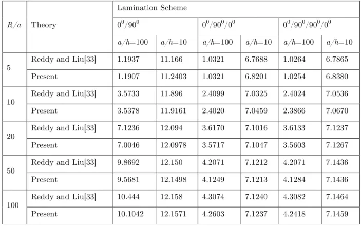
is considered for the analysis. This problem is earlier solved by Reddy and Liu [33]. The lamination schemes are taken as in the pr e-vious example. It is found that the present results are in close agreement with the results of Reddy and Liu [33] based on HSDT. The non-dimensional central displacements are obtained as,w
=
−
wh
3e2
qa
4⎛
⎝⎜
⎞
⎠⎟
10
Table 2 Non-dimensional central deflections of simply supported cross-ply laminated spherical shells under sinusoidally distributed load (a/b=1, Rx=Ry=R)
R/a Theory
Lamination Scheme
00/900 00/900/00 00/900/900/00
a/h=100 a/h=10 a/h=100 a/h=10 a/h=100 a/h=10
5
Reddy and Liu[33] 1.1937 11.166 1.0321 6.7688 1.0264 6.7865
Present 1.1907 11.2403 1.0321 6.8201 1.0254 6.8380
10
Reddy and Liu[33] 3.5733 11.896 2.4099 7.0325 2.4024 7.0536
Present 3.5378 11.9161 2.4020 7.0459 2.3866 7.0670
20
Reddy and Liu[33] 7.1236 12.094 3.6170 7.1016 3.6133 7.1237
Present 7.0046 12.0978 3.5717 7.1047 3.5603 7.1267
50
Reddy and Liu[33] 9.8692 12.150 4.2071 7.1212 4.2071 7.1436
Present 9.5681 12.1498 4.1249 7.1213 4.1284 7.1436
100
Reddy and Liu[33] 10.444 12.158 4.3074 7.1240 4.3082 7.1464
Present 10.1042 12.1571 4.2603 7.1237 4.2418 7.1459
3.1.2.2 Conical shell with different boundary conditions
A laminated (00/900/00) conical shell panel is considered in this example with a slant edge L, radii at top and bottom Rtand Rb, respectively. The shell is subjected to uniform lateral pressure p. 12 X 12mesh is used to discretise the shell. The material properties considered are as follows: EL = 2.0 X 10¹¹ Pa, EL/ET = 2, 10, 20 and 30, G12= G13=0.5 X ET, G23= 0.2 X ET, ν12= ν13 = ν23 = 0.25.
The central deflections (Table 3) based on the present theory were found to be in good agre e-ment with those obtained by Bhaskar and Varadan [3] based on HSDT for clamped boundary conditions. New results for boundary conditions like SSSS, SSCC and SCSC are also presented in Table 3. It can be observed that as the ratio EL/ET increases the deflection values decrease. On
the other hand as the ratio Rb/h is increased from 10 to 100 there is considerable decrease in
Figure 3 Conical Shell panels
Table 3 Non-dimensionalized central deflection w=100 E
Th
3 w/pL4
(
)
of a (00/900/00) conical shell panel (Rt= 0.8Rb, L = Rb, Rb/h=10 )Boundary condition Rb/h Theory
EL/ET
2 10 20 30
CCCC 10
Bhaskar and Varadan [3] 0.3646 0.1270 0.0751 0.0538
Present 0.3612 0.1318 0.0774 0.0551
100 Present 0.0043 0.0015 0.0008 0.0005
SSSS 10 Present 0.8517 0.4946 0.3910 0.3476
100 Present 0.0095 0.0083 0.0077 0.0075
SSCC 10 Present 0.4494 0.1765 0.1131 0.8546
100 Present 0.0062 0.0026 0.0015 0.0011
SCSC 10 Present 0.5718 0.3036 0.2441 0.2206
100 Present 0.0073 0.0053 0.0046 0.0043
3.1.2.3 Cylindrical shell
3.1.2.3.1 Cross-ply cylindrical shell
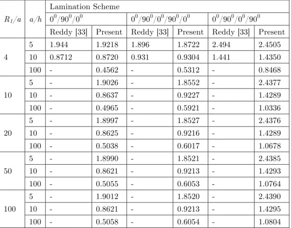
Simply supported three-ply (00/900/00), four-ply (00/900/00/900) and five-ply (00/900/00/900/00) laminated cylindrical shells with R1/a = 4 and b/a = 3 is considered in this example. Taking
sinusoidal variation of loading q=q0sin
π
xa
sin
π
yb
⎛
Table 4 Non-dimensional central deflection w=100 ETw/qhS4
(
)
of simply supportedlaminatedcylindricalshell panel (R1/a = 4, a/h = 10)R1/a a/h
Lamination Scheme
00/900/00 00/900/00/900/00 00/900/00/900
Reddy [33] Present Reddy [33] Present Reddy [33] Present
4
5 1.944 1.9218 1.896 1.8722 2.494 2.4505
10 0.8712 0.8720 0.931 0.9304 1.441 1.4350
100 - 0.4562 - 0.5312 - 0.8468
10
5 - 1.9026 - 1.8552 - 2.4377
10 - 0.8637 - 0.9227 - 1.4289
100 - 0.4965 - 0.5921 - 1.0336
20
5 - 1.8997 - 1.8527 - 2.4376
10 - 0.8625 - 0.9216 - 1.4289
100 - 0.5038 - 0.6017 - 1.0678
50
5 - 1.8990 - 1.8521 - 2.4385
10 - 0.8621 - 0.9213 - 1.4293
100 - 0.5055 - 0.6053 - 1.0764
100
5 - 1.9012 - 1.8520 - 2.4390
10 - 0.8621 - 0.9213 - 1.4295
100 - 0.5058 - 0.6054 - 1.0804
Note: Reddy [33] -Reddy’s higher-order theory [multiplied by a factor (1 + h/2R1) (1 + h/2R2,)].
It is observed in Table 4 that for lower values of thickness ratio (a/h) present results slightly differ from the results presented by Reddy and Liu [33]. This difference may be due to the fact that the deflection results of Reddy and Liu [33] shown in Table 4 are multiplied by a factor (1 + h/2R1) (1 + h/2R2,). Moreover, Reddy and Liu [33] have not included the effect of twist curv a-ture (1/Rxy) in their formulation. The geometry of cylindrical shell is as shown in Figure [4]. It can also be observed that with increasing values of R1/a and a/h the deflections decrease.
The lamination scheme (00/900/00) was found to give lesser deflection compared to other schemes for a/h =10, 100 while for a/h=5, lamination scheme (00/900/00/900/00) is found give
lesser values for the deflections. It is also observed that the anti-symmetric lamination scheme
(00/900/00/900) gives higher results in all the cases.
3.1.2.3.2 Angle-ply cylindrical shell
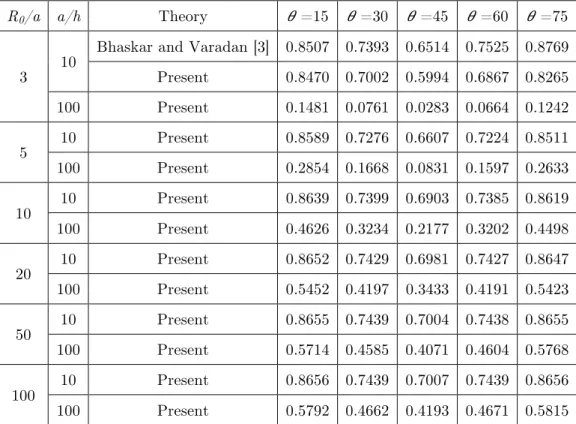
In this example, an angle-ply (�/- � / � /- � / �) cylindrical shell panel of square plan form, simply supported at all edges and subjected to uniform transverse pressure p is considered. Non -dimensional central deflections obtained by using the present model are compared with the corr e-sponding results of Bhaskar and Varadan [3]. It may be observed in Table 5 that there are diffe r-ences between the two results for higher values of ply angles (�). This may be due to the reasons
that the loading considered in the two models are slightly different; and also Bhaskar and Var a-dan [3] have not considered the twist curvature (1/Rxy) in their formulation which may be signifi-cant for angle ply lamination schemes. Some new results are also presented in Table 5. It is o b-served minimum deflection values corresponds to�=45 for all the cases.
Table 5 Non-dimensionalized central deflection w=100 ETh3
/
pa4(
)
of simply supported angle-ply (� /-�/ � /-� /�) cylindricalshell panel.R0/a a/h Theory � =15 �=30 �=45 � =60 �=75
3 10
Bhaskar and Varadan [3] 0.8507 0.7393 0.6514 0.7525 0.8769 Present 0.8470 0.7002 0.5994 0.6867 0.8265
100 Present 0.1481 0.0761 0.0283 0.0664 0.1242
5
10 Present 0.8589 0.7276 0.6607 0.7224 0.8511
100 Present 0.2854 0.1668 0.0831 0.1597 0.2633
10
10 Present 0.8639 0.7399 0.6903 0.7385 0.8619
100 Present 0.4626 0.3234 0.2177 0.3202 0.4498
20
10 Present 0.8652 0.7429 0.6981 0.7427 0.8647
100 Present 0.5452 0.4197 0.3433 0.4191 0.5423
50
10 Present 0.8655 0.7439 0.7004 0.7438 0.8655
100 Present 0.5714 0.4585 0.4071 0.4604 0.5768
100
10 Present 0.8656 0.7439 0.7007 0.7439 0.8656
100 Present 0.5792 0.4662 0.4193 0.4671 0.5815
3.1.2.4 Hypar shell
In this example cross-ply laminated hypar shells having four lamination schemes of (00/900), (00/900/900/00), (00/900/00/900) and (00/900/00/900/00)with simply supported as well as clamped
twist curvature of the hypar shell. The results are compared with those obtained by Pradyumna and Bandyopadhyay [31] and found to match very well with each other. Some new results are
also presented. Lamination scheme 00/900/900/00 is found to give lesser deflections in all cases especially in case of clamped boundary (CCCC) conditions. The geometry of hypar shell is as
shown in Figure [5].
Figure 5 Perspective view of hypar shell panel
Table 6 Non-dimensional central deflection ofcross-ply laminatedhypar shell panel
c/a Theory
Lamination scheme
00/900 00/900/900/00 00/900/00/900 00/900/00/900/00 a/h =
100
a/h =
10
a/h =
100
a/h =
10
a/h =
100
a/h =
10
a/h =
100
a/h =
10 SSSS-uniform
0
Pradyumna and Bandyopadhyay
[31]
16.9763 - 6.8436 - 8.1137 - - -
Present 16.4961 19.1698 6.8008 11.0546 8.0119 10.6923 6.8579 9.8175
0.05
Pradyumna and Bandyopadhyay
[31]
2.3744 - 1.9629 - 2.0922 - - -
Present 2.3696 17.9858 1.9556 10.6522 2.0861 10.3190 1.9841 9.5001
0.1
Pradyumna and Bandyopadhyay
[31]
0.6193 - 0.5972 - 0.6252 - - -
Present 0.6188 15.1714 0.5966 9.6030 0.6247 9.3402 0.6101 8.6616
0.15
Pradyumna and Bandyopadhyay
[31]
0.2610 - 0.2638 - 0.2767 - - -
Present 0.2608 12.0271 0.2637 8.2471 0.2765 8.0642 0.2714 7.5492
0.2
Pradyumna and Bandyopadhyay
[31]
0.1388 - 0.1434 - 0.1504 - - -
Table 6 (continued)
SSSS-sinusoidal
0
Pradyumna and Bandyopadhyay
[31]
10.6524 - 4.3441 - 5.0857 - - -
Present 10.3521 12.1582 4.3160 7.1463 5.0214 6.8644 4.3216 6.3447
0.05
Pradyumna and Bandyopadhyay
[31]
1.6785 - 1.3511 - 1.3866 - - -
Present 1.6714 11.4372 1.3453 6.9039 1.3819 6.6391 1.3310 6.1540
0.1
Pradyumna and Bandyopadhyay
[31]
0.5672 - 0.4966 - 0.4781 - - -
Present 0.5654 9.7232 0.4956 6.2718 0.4771 6.0483 0.4781 5.6491
0.15
Pradyumna and Bandyopadhyay
[31]
0.3167 - 0.2716 - 0.2545 - - -
Present 0.3158 7.8083 0.2712 5.4550 0.2539 5.2783 0.2575 4.9799
0.2
Pradyumna and Bandyopadhyay
[31]
0.2180 - 0.1800 - 0.1680 - - -
Present 0.2173 6.1563 0.1797 4.6336 0.1675 4.4964 0.1698 4.2870 CCCC-uniform
0
Pradyumna and Bandyopadhyay
[31]
3.9672 - 1.4859 - 1.7894 - - -
Present 3.9276 5.8701 1.4767 4.8050 1.7738 4.0677 1.4785 4.0236
0.05
Pradyumna and Bandyopadhyay
[31]
1.3371 - 0.8459 - 0.9640 - - -
Present 1.3349 5.7104 0.8432 4.6902 0.9606 3.9857 0.8585 3.9424
0.1
Pradyumna and Bandyopadhyay
[31]
0.3901 - 0.3451 - 0.3791 - - -
Present 0.3923 5.2770 0.3455 4.3748 0.3797 3.7574 0.3588 3.7162
0.15
Pradyumna and Bandyopadhyay
[31]
0.1576 - 0.1613 - 0.1732 - - -
Present 0.1589 4.6781 0.1619 3.9289 0.1741 3.4269 0.1693 3.3887
0.2
Pradyumna and Bandyopadhyay
[31]
0.0805 - 0.0879 - 0.0917 - - -
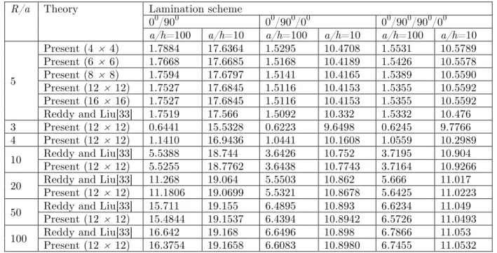
Table 6 (continued)
CCCC-sinusoidal
0
Pradyumna and Ba
n-dyopadhyay [31] 2.8703 - 1.0967 - 1.2944 - - -
Present 2.8445 4.2399 1.0909 3.4731 1.2847 2.9326 1.0819 2.9112
0.05
Pradyumna and Ba
n-dyopadhyay [31] 1.0168 - 0.6440 - 0.7138 - - -
Present 1.0140 4.1300 0.6418 3.3949 0.7115 2.8770 0.6430 2.8561
0.1
Pradyumna and Ba
n-dyopadhyay [31] 0.3335 - 0.2826 - 0.2988 - - -
Present 0.3337 3.8316 0.2424 3.1800 0.2989 2.7220 0.2853 2.7024
0.15
Pradyumna and Ba
n-dyopadhyay [31] 0.1524 - 0.1433 - 0.1484 - - -
Present 0.1526 3.4189 0.1433 2.8757 0.1485 2.4973 0.1451 2.4797
0.2
Pradyumna and Ba
n-dyopadhyay [31] 0.0852 - 0.0837 - 0.0836 - - -
Present 0.0853 2.9694 0.0837 2.5350 0.0856 2.2380 0.0847 2.2225
3.2 Analysis of laminated composite skew shell
In this section some examples of laminated composite skew hypar and cylindrical shells are stu d-ied using the present FE model based on HSDT.
3.2.1 Skew Hypar shell
Skew hypar shells (b/a =1) having different boundary conditions are considered in this example taking three different lamination schemes (00/900, 00/900/00, 00/900/00/900) and varying c/a ratio (0.0, 0.1, 0.2) as well as a/h ratio (10, 100). Skew angles are varied from 00 to 450. Non
-dimensional central deflections ( ) and stresses obtained by using the present FE
model are shown in Table 7 and Table 8 respectively. The present results for c/a = 0, represen t-ing plate geometry are compared with the correspondt-ing results obtained by Chakrabartiet. al [5] for simply supported skew composite plates. It may be observed from Table 7 and 8 that the pr e-sent results are matching quite well with those obtained by Chakrabarti et al.. [5]. The pree-sent model is therefore used to generate other new results. It is observed that the deflection values tend to decrease with increase in c/a ratio as well as a/h ratio. In this case of skew hypar shell,
lamination scheme (00/900/00/900) was found to give minimum central deflections. Thin shells (a/h = 100) with clamped boundary condition (CCCC) are found to give minimum deflections in all the cases listed in Table 7. Non-dimensional stresses for the same problem of hypar shell are
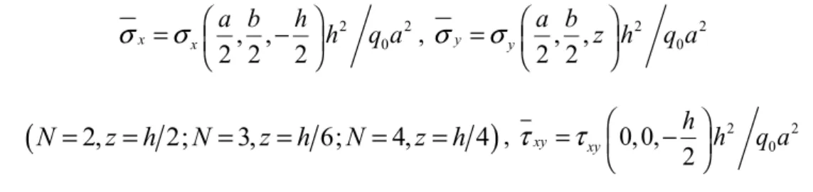
also presented in Table 8 (a/h = 100). In-plane normal stresses and transverse shear stress are non-dimensionalized using following factors:
3 3 2 4 0
10
wh E
w
q a
⎛
⎞
=
⎜
⎟
,
,
Table 7 Non-dimensional central deflections of a laminated composite hypar shell panel subjected to uniform loading (b/a =1)
Boundary co
n-dition c/a
Skew angle
Laminationscheme
00/900 00/900/00 00/900/00/900 a/h
=10 a/h=100 a/h=10 a/h=100 a/h=10 a/h=100
SSSS
0.0
00 19.2188 16.9637 10.9812 6.7064 10.6967 8.1081
- - 10.91171 6.7168 - -
150 16.5631 14.2388 10.4300 6.4294 9.4613 6.8517
- - 10.36691 6.4392 - -
300 10.7202 8.6394 8.6613 5.4608 6.4902 4.1722
- - 8.62171 5.4708 - -
450 5.2223 3.7667 5.7181 3.6190 3.4184 1.8098
- - 5.71051 3.6333 - -
0.1
00 15.1721 0.6188 9.4652 0.5680 9.3404 0.6247 150 13.9406 0.5797 8.9882 0.5505 8.4446 0.5890
300 9.8189 0.5580 7.6182 0.5364 6.0453 0.5487
450 5.0687 0.5756 5.2683 0.5430 3.3177 0.5016
0.2
00 9.3148 0.1384 6.7769 0.1358 6.7681 0.1502 150 8.9257 0.1237 6.4289 0.1326 6.2558 0.1387
300 7.1747 0.1203 5.6522 0.1296 4.8556 0.1325
450 4.3850 0.1364 4.3095 0.1399 2.9727 0.1416
CCCC
0.0
00 6.2088 3.9552 5.2198 1.4184 4.3159 1.7830
150 5.6912 3.5419 4.9871 1.3899 4.0084 1.6007 300 4.2922 2.4602 4.2252 1.2692 3.1558 1.1183 450 2.5206 1.1936 2.8971 0.9582 2.0114 0.5458
0.1
00 5.3198 0.3923 4.4877 0.3269 3.8027 0.3797
150 4.9039 0.3916 4.3088 0.3268 3.5443 0.3712 300 3.7603 0.3832 3.7114 0.3263 2.8215 0.3388 450 2.2386 0.3395 2.6144 0.3135 1.8189 0.2582
0.2
00 4.0479 0.0810 3.4924 0.0882 3.0735 0.0924
150 3.7987 0.0828 3.3809 0.0879 2.8991 0.0933 300 3.0725 0.0879 3.0008 0.0879 2.3943 0.0951
450 1.9781 0.0945 2.2423 0.0909 1.6315 0.0927
2 2
0
,
,
2 2
2
x x
a b
h
h
q a
σ
=
σ
⎛
⎜
−
⎞
⎟
⎝
⎠
2 2
0
,
,
2 2
y y
a b
z h
q a
σ
=
σ
⎛
⎜
⎞
⎟
⎝
⎠
(
N
=
2,
z
=
h
2;
N
=
3,
z
=
h
6;
N
=
4,
z
=
h
4
)
2 2 00, 0,
2
xy xyh
h
q a
τ
=
τ
⎛
⎜
−
⎞
⎟
Table 7 (continued)
SCSC
0.0
00 9.9870 7.2803 7.2947 2.7499 6.3726 3.3415
150 8.9476 6.3348 6.9529 2.6690 5.8152 2.9199
300 6.4114 4.2032 5.8512 2.3629 4.3639 1.9459 450 3.5369 1.9953 3.9673 1.6895 2.5920 0.9269
0.1
00 8.2657 0.4209 6.2159 0.3801 5.5637 0.4322
150 7.5967 0.4223 5.9545 0.3798 5.1347 0.4255 300 5.7087 0.4322 5.1217 0.3889 3.9584 0.4085 450 3.2650 0.4374 3.6102 0.4034 2.4162 0.3546
0.2
00 5.6746 0.0827 4.5737 0.0928 4.2349 0.0968
150 5.3960 0.0856 4.4209 0.0923 3.9914 0.0984
300 4.4532 0.0935 3.9627 0.0946 3.2720 0.1035
450 2.8774 0.1103 3.0405 0.1068 2.1736 0.1122 1
Results of these rows corresponds to Chakrabarti et al. [5].
Table 8 Non-dimensional stresses of a laminated composite hypar shell panel subjected to uniform loading (b/a =1, a/h = 100)
c/a Skew angle
Laminationscheme
00/900 00/900/00 00/900/00/900
σ
xσ
y
τ
xyσ
xσ
yτ
xyσ
xσ
yτ
xySimplysupported (SSSS)
0.0
00 1.0762 -1.0762 -0.0940 0.8094 0.1937 -0.0432 0.7374 0.7005 -0.0447 150 0.9496 -0.9598 -0.0473 0.7757 0.2196 -0.0270 0.6464 0.6262 -0.0169 300 0.6435 -0.7258 -0.0053 0.6597 0.2807 -0.0136 0.4344 0.4696 -0.0014 450 0.3200 -0.4969 0.0027 0.4482 0.3193 -0.0033 0.2158 0.3190 0.0007
0.1
00 0.0244 -0.0244 -0.0237 0.0614 0.0051 -0.0234 0.0448 0.0425 -0.0229 150 0.0047 -0.0248 -0.0058 0.0472 0.0037 -0.0047 0.0288 0.0424 -0.0034 300 -0.0209 -0.0334 -0.0029 0.0284 0.0094 -0.0029 0.0094 0.0505 -0.0014 450 -0.0390 -0.0681 -0.0014 0.0123 0.0330 -0.0031 -0.0019 0.0810 -0.0014
0.2
00 0.0019 -0.0019 -0.0109 0.0123 -0.0012 -0.0112 0.0060 0.0057 -0.0110 150 -0.0079 -0.0016 -0.0028 0.0051 -0.0009 -0.0021 -0.0029 0.0065 -0.0016 300 -0.0211 -0.0024 -0.0017 -0.0054 -0.0005 -0.0015 -0.0152 0.0089 -0.0008 450 -0.0379 -0.0112 -0.0009 -0.0161 0.0046 -0.0018 -0.0273 0.0201 -0.0009
Clamped (CCCC)
0.0
00 0.4036 -0.4036 0 0.2788 0.0406 0 0.2592 0.2448 0 150 0.3647 -0.3897 0 0.2728 0.0529 0 0.2337 0.2367 0 300 0.2651 -0.3410 0 0.2479 0.0880 0 0.1688 0.2077 0 450 0.1471 -0.2508 0 0.1879 0.1282 0 0.0932 0.1529 0
0.1
00 0.0134 -0.0134 0 0.0530 -0.0045 0 0.0369 0.0348 0 150 0.0126 -0.0179 0 0.0510 -0.0055 0 0.0347 0.0383 0 300 0.0148 -0.0329 0 0.0486 0.0018 0 0.0328 0.0500 0 450 0.0202 -0.0604 0 0.0450 0.0244 0 0.0310 0.0658 0
0.2
Table 8 (continued)
Simply supported-Clamped (SCSC)
0.0
00 0.5591 -0.5591 -0.0609 0.4056 0.0840 -0.0273 0.3686 0.3532 -0.0282
150 0.4948 -0.5262 -0.0331 0.3929 0.1036 -0.0176 0.3221 0.3364 -0.0116
300 0.3534 -0.4368 -0.0048 0.3466 0.1493 -0.0095 0.2261 0.2834 -0.0013 450 0.1856 -0.3123 0.0013 0.2495 0.1916 -0.0026 0.1181 0.2076 0.0004
0.1
00 0.0047 -0.0125 -0.0191 0.0453 -0.0148 -0.0182 0.0248 0.0231 -0.0158
150 -0.0079 -0.0193 -0.0078 0.0356 -0.0180 -0.0066 0.0132 0.0255 -0.0042 300 -0.0250 -0.0359 -0.0028 0.0223 -0.0092 -0.0035 0.0001 0.0395 -0.0011
450 -0.0375 -0.0642 -0.0002 0.0089 0.0214 -0.0019 -0.0069 0.0677 -0.0323
0.2
00 -0.0052 0.0044 -0.0106 0.0051 -0.0057 -0.0099 -0.0028 -0.0029 -0.0089
150 -0.0109 0.0037 -0.0044 0.0005 -0.0083 -0.0037 -0.0087 -0.0024 -0.0025
300 -0.0210 -0.0003 -0.0018 -0.0071 -0.0097 -0.0020 -0.0175 0.0013 -0.0008 450 -0.0357 -0.0110 -0.0003 -0.0177 -0.0042 -0.0012 -0.0267 0.0142 -0.0003
3.2.2 Skew Cylindrical shell
In this example, Cross-ply laminated skew cylindrical shells (b/a=3) having symmetric lamination scheme as (00/900/00) and anti-symmetric lamination schemes as (00/900), (00/900/00/900) with simply supported and clamped boundary conditions are considered. The skew angle is varied from 00 to 450. These shells are subjected to uniform loading with varying R/a (3, 10, 100) as well as
a/h (10, 100) ratios.
In Table 9 the values of non-dimensional central deflections
( )
w
of three different laminationschemes are presented for different skew angles. It can be observed that the deflection values d e-crease with ine-crease in skew angle. Also there is not much effect of R/a ratio on the deflection values. The clamped boundary condition is more effective in reduction of deflection values as compared to the simply supported boundary condition. The reduction in deflection with increase ina/h ratio from 10 to 100 makes thin shells more effective. The superiority of (00/900/00) lam i-nation scheme is observed in all the cases mentioned in Table 9.
Table 9 Non-dimensional central deflections of a laminated composite cylindrical shell panel subjected to uniform loading (b/a =3)
Boundary cond
i-tion R/a
Skew
angle
Lamination scheme
00/900 00/900/00 00/900/00/900
a/h=10 a/h=100 a/h=10 a/h=100 a/h=10 a/h=100
SSSS
3
00 38.6423 17.5678 11.2634 6.2711 20.1208 11.0884
150 35.7127 8.7441 11.0503 4.3794 18.8462 6.4675
300 26.3440 2.4594 10.0582 1.7653 14.4127 2.0799
450 13.2141 0.4843 7.2277 0.4157 7.6007 0.4280
10
00 38.4591 32.2695 10.9839 6.5265 19.8321 14.8302
150 35.6285 27.1971 10.8545 6.2772 18.7313 13.2245
300 25.9215 15.8484 10.2259 5.1350 14.6473 8.4976
450 12.2178 6.1815 8.2528 2.6949 7.9607 3.3300
100
00 38.5372 34.3715 10.9568 6.48221 19.8325 15.0855
150 35.4921 31.8843 10.8352 6.4357 18.7187 14.3902
300 25.1606 22.6344 10.2421 6.2211 14.5660 11.1852 450 11.2650 9.9188 8.3683 5.3999 7.7924 5.5613
CCCC
3
00 5.4914 0.1277 3.2664 0.0923 4.3743 0.1242
150 5.3737 0.1271 3.2430 0.0921 4.2795 0.1239
300 4.7629 0.1251 3.1225 0.0913 3.7558 0.1224 450 3.1886 0.1205 2.6770 0.0891 2.5287 0.1154
10
00 9.3282 1.1821 4.8846 0.6000 6.6049 0.9538
150 8.9780 1.1732 4.8322 0.5977 6.3762 0.9484
300 7.3744 1.1221 4.5641 0.5872 5.2632 0.8985
450 4.1901 0.9215 3.6614 0.5508 3.1421 0.6729
100
00 10.0241 6.3319 5.1342 1.3081 6.9555 2.8344
150 9.6189 6.1223 5.0764 1.2977 6.7008 2.7854
300 7.7994 5.0049 4.7805 1.2528 5.4809 2.3783
450 4.3241 2.5959 3.7980 1.1056 3.2191 1.2628
SCSC
3
00 17.6312 6.2102 7.3655 2.3365 10.9063 4.0331
150 16.6497 4.0103 7.2339 1.9001 10.3625 2.8937 300 12.9507 1.2835 6.5332 0.9088 8.1242 1.0771
450 6.8585 0.2697 4.5251 0.2394 4.4016 0.2403
10
00 17.7013 12.6187 7.2659 2.6306 10.8758 5.7734
150 16.8148 11.2045 7.1814 2.5585 10.4146 5.3678
300 13.1846 7.0018 6.7511 2.1823 8.4134 3.7366
450 6.9278 2.7386 5.3537 1.2625 4.8174 1.5215
100
00 17.7372 13.5193 7.2558 2.6230 10.8830 5.8865
150 16.8055 12.8839 7.1757 2.6014 10.4203 5.7363
300 12.9510 9.9939 6.7728 2.5095 8.3959 4.7387
Table 10 Non-dimensional stresses of laminated cylindrical shell subjected to sinusoidal loading (b/a=3, R/a=4)
a/h Skew angle
Lamination scheme
00/900 00/900/00 00/900/00/900
σ
xσ
y
τ
xyσ
xσ
yτ
xyσ
xσ
yτ
xySimply Supported (SSSS)
10
00 1.6878 0.2719 0.0521 0.6930 0.0608 0.0141 1.1007 0.1842 0.0257
- - - 0.69852 0.0603 0.0140 1.100 0.1846 0.02573 150 0.5902 0.1366 0.0133 0.2686 0.0395 0.0054 0.3921 0.0096 0.0034
300 0.6109 0.3359 0.0009 0.3642 0.1074 0.0019 0.4122 0.2199 0.0035
450 0.4967 0.4957 0.0015 0.4403 0.2503 0.0097 0.3339 0.3451 0.0012
100
00 0.9797 0.3860 0.0708 0.5553 0.1283 0.0202 0.8029 0.2496 0.0404
150 0.1857 0.0875 0.0096 0.1763 0.0425 0.0047 0.1956 0.0728 0.0051
300 0.1215 0.0738 0.0025 0.1495 0.0496 0.0025 0.1170 0.0754 0.0011 450 0.0318 0.0507 0.0009 0.1349 0.0469 0.0016 0.0443 0.0680 0.0003
Clamped (CCCC)
10
00 0.2937 0.0547 0 0.3510 0.0161 0.0054 0.2022 0.0529 0 150 0.0991 0.0330 0 0.1344 0.0125 0.0014 0.0688 0.0309 0
300 0.1613 0.1197 0 0.2040 0.0416 0 0.1124 0.0959 0
450 0.1719 0.2246 0 0.2727 0.1256 0 0.1237 0.1672 0
100
00 0.0070 0.0042 0 0.0810 0.0014 0 0.0099 0.0038 0
150 0.0215 0.0034 0 0.0305 0.0001 0 0.0116 0.0008 0
300 0.0128 0.0028 0 0.0509 0.0021 0 0.0023 0.0054 0
450 0.0052 0.0111 0 0.0819 0.0045 0 0.0043 0.0224 0
Simply Supported-Clamped (SCSC)
10
00 0.9357 0.1408 0.0333 0.4399 0.0379 0.0122 0.6434 0.1115 0.0189 150 0.3967 0.1098 0.0099 0.1968 0.0359 0.0041 0.2733 0.0804 0.0026
300 0.3541 0.1589 0.0010 0.2231 0.0297 0.0021 0.2389 0.1084 0.0007
450 0.3238 0.3402 0.0003 0.3240 0.1523 0.0013 0.2161 0.2310 0.0005
100
00 0.44612 0.1327 0.0482 0.2829 0.0423 0.0145 0.3849 0.0895 0.0280 150 0.0891 0.0652 0.0075 0.1163 0.0306 0.0031 0.1139 0.0545 0.0038
300 0.0839 0.0264 0.0028 0.0898 0.0268 0.0021 0.0721 0.0139 0.0016
450 0.0002 0.0034 0.0017 0.0989 0.0027 0.0019 0.0093 0.0196 0.0013 2Results of this row corresponds to Xiao-ping [39]
3.2.2.2 Angle-ply laminated skew cylindrical shell
Angle-ply laminated (450/-450/450/-450) skew cylindrical shell (b/a =3) is considered in this e
x-ample. The shell is subjected to uniform loading with different boundary conditions such as sim p-ly supported and clamped. The skew angle is varied from 00to 450. The R/a (3, 10, 100) as well as a/h (10, 100) ratios are also varied.
Variation of non-dimensional central deflection (Figures 6a-6e) and in-plane normal stress (Fi
g-ures 7a-7e) with skew angle is presented [Figures (a, b): Simply supported, Figures (c, d):
clamped boundary condition, the in-plane shear stress was found to be zero for all the cases; var
i-ation of in-plane shear stress with skew angle is shown (Figures 8a-8d) only for two boundary
conditions [Figure 8(a, b): Simply supported, 8(c, d): Simply supported-clamped boundary cond i-tions]. From the figures it can be observed that the deflection and stresses follow the expected general trend. With increase in R/a ratio, central deflection values differ significantly in case of
thin shells (a/h = 100) as compared to those for thick shells (a/h = 10). Deflection and stresses tend to decrease as the skew angle increases. In Figures 8 it can be observed that in-plane shear
stresses tend to attain minimum value approximately at skew angle of 300.
6(a) 6(b)
6(c) 6(d)
6(e) 6(f)
Figure 6 Variation of non-dimensional central deflections
( )
w
of laminated angle ply skew composite cylindrical shell
7(a) 7(b)
7(c) 7(d)
7(e) 7(f)
Figure 7 Variation of non-dimensional in-plane normal stress (
σ
x) of laminated angle ply skew composite cylindrical shell8(a) 8(b)
8(c) 8(d)
Figure 8Variation of non-dimensional in-plane shear stress
τ
xy of laminated angle ply skew composite cylindrical shell with skewangles
4 CONCLUSIONS
In this paper, a new finite element model has been developed for the analysis of skew composite shells based on higher order shear deformation theory (HSDT) using a C0 formulation. In this
model there is no need to include any shear correction factor. Three radii of curvatures including
the cross curvature effects are also considered in the FE formulation which accounts for twisting effect of the geometry. Different shell forms considered in this study include spherical, conical, cylindrical and hypar shells. It is observed there is no result available in the literature on the present problem of skew composite shell. Therefore, many new results are generated on the static
response of laminated composite skew shells considering different geometry, boundary conditions,
ply orientation, loadings and skew angles which should be useful for future research.


![Table 6 (continued) CCCC - sinusoidal 0 Pradyumna and Ba n-dyopadhyay [31] 2.8703 - 1.0967 - 1.2944 - - - Present 2.8445 4.2399 1.0909 3.4731 1.2847 2.9326 1.0819 2.9112 0.05 Pradyumna and Ba n-dyopadhyay [31] 1.0168 - 0.6440 -](https://thumb-eu.123doks.com/thumbv2/123dok_br/18884733.423550/18.892.115.817.124.418/table-continued-sinusoidal-pradyumna-dyopadhyay-present-pradyumna-dyopadhyay.webp)