P. R. M. Lyra
R. de C. F. de Lima
and C. S. C. Guimarães
Departamento de Engenharia Mecânica – UFPE Av. Acadêmico Hélio Ramos, S/N 50740-530 Recife, PE. Brazil [email protected] [email protected] [email protected]
D. K. E. de Carvalho
Departamento de Engenharia Civil – UFPE Av. Acadêmico Hélio Ramos, S/N 50740-530 Recife, PE. Brazil [email protected]
An Edge-Based Unstructured Finite
Volume Procedure for the Numerical
Analysis of Heat Conduction
Applica-tions
In recent years, there has been a significant level of research on the application of un-structured mesh methods to the simulation of a variety of engineering and scientific prob-lems. Great progress has been achieved in such area and one of the most successful meth-odologies consists on the use of the Finite Volume Method (FVM). The unstructured FV formulation is very flexible to deal with any kind of control volume and therefore any kind of unstructured meshes, which are particularly important when complex geometries or automatic mesh adaptation are required. In this article, an unstructured finite volume ver-tex centered formulation, which was implemented using an edge-based data structure, is deduced and detailed for the solution of heat conduction problems. The numerical formu-lation is initially described considering a tri-dimensional model and latter particularized for bi-dimensional applications using triangular meshes. The presented procedure is very flexible and efficient to solve potential problems. It can also be extended to deal with a broader class of applications, such as models involving convection-diffusion-reaction terms, after considering the appropriate discretization of the convection-type term. In or-der to demonstrate the potentiality of the method, some model problems are investigated and the results are validated using analytical or other well-established numerical solu-tions.
Keywords: Finite volume method, unstructured mesh, edge based data structure, heat
transfer
Introduction
Whenever analyzing numerical applications that involve com-plex geometries the adoption of methods capable to deal with un-structured meshes is very attractive and highly recommended (AGARD Report 787, 1992). Within such class of methods the most frequently used are the finite element method (FEM), (Zienkiewicz and Morgan, 1983) and the finite volume method (FVM), (Barth, 1992). The FVM is very flexible to deal with any kind of control volumes and, consequently, any kind of unstructured meshes includ-ing dual meshes. Finite volume methods are usually either a node/vertex centered, where the unknowns are defined at the nodes of the mesh, or element/cell centered where the unknowns are de-fined within the element, usually at the element’s centroid. Both options have advantages and disadvantages, but in two-dimensional applications all of them have basically the same computational cost, which is proportional to the number of edges of the mesh. However, the node-centered formulation has a strong connection with an edge-based finite element formulation, when linear triangular (tetrahedral) elements are used, and requires less memory and computations when extended for three-dimensional tetrahedral meshes, (Barth, 1992, Peraire et al., 1993 and Sorensen et al., 2001). The adoption of unstructured grids implies the storage of mesh topology informa-tion (connectivities), increasing the use of computer memory and indirect addressing to retrieve local information required by the solver. In order to reduce indirect addressing, CPU time and mem-ory requirements (Barth, 1992, Peraire et al., 1993 and Lyra, 1994), an edge-based data structure is adopted. This data structure also enables a straightforward implementation of different types of finite difference discretization, such as upwind-biased schemes in the context of unstructured algorithms, when dealing with CFD (Com-putational Fluid Dynamics) problems, (Peraire et al., 1993 and Lyra et al., 1994).1
Paper accepted January, 2004. Technical Editor: Atila P. Silva Freire.
In this paper, the vertex centered finite volume formulation us-ing median dual control volumes is implemented usus-ing an edge-based data structure, (Barth, 1992, Sorensen et al., 1999 and Lyra et al., 2002). The complete formulation is deduced and detailed for the solution of heat conduction problems. In two dimensional (2-D) models, triangular, quadrilateral or mixed meshes can be directly used, and the same happens when dealing with three dimensional (3-D) models, where tetrahedral, hexahedral, pyramids, prisms and mixed meshes can be adopted. We derive the FV discretization of a transient potential problem subject to different types of boundary conditions (Dirichlet, Neumann, and Cauchy) and to some non-conventional loads, considering also systems with multi-materials.
This paper is organized as follows: after these initial considera-tions, the physical-mathematical model considered is described. Then, the discrete spatial formulation adopted is fully presented. Some important implementation aspects are discussed and several simple model problems are analyzed to validate and to study the performance of the whole procedure. Finally, some concluding comments are presented and the potentiality of the described ap-proach is highlighted.
Mathematical Model
Using the energy conservation law we can derive the partial dif-ferential equation that governs transient heat transfer in a stationary continuous medium,
in x Τ ρ ∂ = − +∂ ∂∂ j Ω
j
q T
c S
t x . (1)
varying from one to the number of spatial dimensions, and
] t , t
[ i f
=
Τ represents the time interval of integration.
The constitutive relation between the conductive heat flux and the temperature gradient is given by Fourier’s law,
j j j x T k q ∂∂ −
= , (2)
in which kj is the thermal conductivity in xj direction. For simplicity, the medium is considered either orthotropic or isotropic with , cρ and k constants. j
Equation (1) represents a boundary-initial value problem and must be subjected to boundary and initial conditions. The boundary conditions of interest can be of three different types:
a) A prescribed temperature T over a portion of the boundary ΓD, i.e., Dirichlet boundary condition:
Τ
x in ΓD
T
T= , (3)
b) A prescribed normal heat flux qn over ΓN, also known as Neumann boundary condition:
N in x Τ
j j n
q n q
− = Γ , (4)
in which nj are the outward normal direction cosines.
c) A mixed type boundary condition over ΓC, called Cauchy or Robin boundary condition:
R ( ) in x Τ
j j n a
q n q αΓ T T
− = + − Γ , (5)
with αΓ representing the film coefficient and Ta being the bulk fluid temperature.
Finally, an initial distribution of the temperature Ti must be known at an initial time stage ti, and the initial condition is ex-pressed by: t t and n
Ω = i
=T i
T i . (6)
Equations (1) to (6) fully describe our mathematical model, which governs heat conduction in a stationary medium.
Finite Volume Formulation
In this section, the majority of the numerical formulation adopted is presented without reference to a particular type of mesh or spatial dimension. The formulation is completed by assuming a two dimensional computational domain discretized into an unstruc-tured assembly of triangular elements. The time discretization adopted is the simple first-order accurate Euler-forward procedure. Such scheme is just first order accurate in time and the ∆t must be chosen according to a stability condition (Zienckiewicz and Morgan, 1983). Other alternatives, such as the generalized trapezoidal method (Zienckiewicz and Morgan, 1983 and Lyra, 1994), multi-stage Runge-Kutta scheme (Lyra, 1994) or schemes involving more than two time intervals (Sorensen, 2001) can be implemented if higher-order time accuracy is required.
The mathematical model presented in previous section repre-sents an example of potential problem and therefore a broad variety of applications governed by similar models can be solved using the numerical procedure to be described in this section.
Spatial Discretization
The integral form of the potential problem given by Eq. (1) is written as,
Ω Ω Ω
ρ ∂∂ Ω= − ∂∂ Ω+ Ω
∫
∫
j∫
j
q T
c d d Sd
t x , (7)
or alternatively by the use of the divergence theorem,
Ω Γ Ω
ρ ∂∂ Ω= − Γ+ Ω
∫
∫
j j∫
T
c d q n d Sd
t , (8)
where Ωdenotes an arbitrary control volume, with closed boundary Γ .
The computational domain is discretized into an unstructured assembly of elements. Then Eq. (8) is applied over each control volume in the mesh. So the volume integrals of (8) can be computed over the control volume surrounding node I as
I I I I V t T c V t T c d t T c I ∂ ∂ ≅ ∂ ∂ ≅ ∂ ∂ ∧
∫
Ω ρ ρρ
Ω
, (9)
and I IV S Sd I ≅
∫
ΩΩ , (10)
where VI is the volume of the control volume, TˆI and SI represent the numerically calculated temperature and source term at node I, respectively. The assumption of ρ andcbeing constants was used in previous approximations.
The boundary integral presented in Eq. (8) is computed over the boundary of the control volume that surrounds node I using an edge-based representation of the mesh, i.e.,
( ) ( ) L L L L I
j j
j j
j j IJ IJ IJ IJ
L L
ˆ ˆ
q n d C q Ω D q Γ
Γ
Γ ≅
∑
+∑
∫
, (11)for a general flux qj. In Equation (11) j IJL
C denotes the coefficient
that must be applied to the approximate edge value of the flux ( )
L
j IJ
ˆq Ω
in the xj direction to obtain the contribution made by the edge L to node I. JL represents the node connected to node I through edge L. In addition, IJj
L
D represents the boundary edge coefficient that must
be applied to the boundary edge flux ( )
L
j IJ
ˆq Γ when the edge L lies on the boundary. These coefficients can be readily computed and this will be detailed afterwards. The first summation in Eq. (11) extends over all edges L in the mesh which are connected to node I, and the second summation is non-zero only when node I is on the boundary and extends over all boundary edges that are connected to node I.
Considering the approximations given by Eqs. (9), (10) and (11), the semi-discrete formulation of Eq. (8) can be conveniently expressed as:
( ) ( )
ˆ
ˆ ˆ
L L L L
j j
j j
I
I IJ IJ IJ IJ I I
L L
dT
c V C q D q S V
dt
Ω Γ
ρ = −⎛⎜⎜ + ⎞⎟⎟+
The approximation of the value of the edge flux ( )
L
j IJ
ˆq Ω is com-puted using the midpoint rule, or simple arithmetic average:
( ) L L j j I J j IJ ˆ ˆ q q ˆq 2
Ω = + . (13)
To compute the boundary edge flux ( )
L
j IJ
ˆq Γ we have considered a linear variation of the flux over edge IJL:
( )
(
L)
L j j I J j IJ ˆ ˆ 3q q ˆ q 4Γ = + . (14)
Alternatively, a finite volume fashion approximation could be used, which would consider the value of the flux constant inside the
control volume and compute ( )
L
j IJ
ˆq Γ as the nodal value ˆqIj. Both options gave good results for the test cases studied and further in-vestigation is required to favor one of them.
In order to compute the edge fluxes described by Eqs. (13) and (14) we need to know the nodal values of the fluxes and so the nodal values of the temperature gradients. By adopting the divergence theorem and the approximation used to compute volume integrals over a control volume surrounding node I (e.g. Eq. (10)), we have:
∫
∫
∂∂ = I I d Tn d x T j j Γ Ω ΓΩ and ˆ
I I I j j T T d V x x Ω
∂ Ω ≅∂
∂ ∂
∫
. (15)From previous expressions and using the same approximation adopted to compute the boundary integral in Eq. (11), we get the approximate nodal gradients through:
( ) ( )
ˆ
ˆ ˆ ˆ
L L L L I
j j
I
I j IJ IJ IJ IJ
j L L
T
V Tn d C T D T
x
Ω Γ
Γ
∂ ≅ Γ ≅ +
∂
∫
∑
∑
. (16)Similarly to the computation of the edge fluxes described in
Eqs. (13) and (14), the edge values of the temperature, ˆ( )
L
IJ
T Ω and
( )
ˆ
L
IJ
TΓ , are calculated by:
( ) ( )
(
)
ˆ ˆ ˆ 2 ˆ ˆ 3 ˆ 4 L L L L I J IJ I J IJ T T T T T T Ω Γ + = + = . (17)The use of Eq. (16) to compute the gradients implies that the discretization of the diffusion term in Eq. (12) involves information from two layers of points surrounding the point I under considera-tion. Furthermore, if uniform structured quadrilateral (or hexahe-dral) meshes are adopted, the values computed at a given node are uncoupled from the values of those nodes directly connected to it. This fact may cause “checker-boarding” or “odd-even” oscillations (Lyra, 1994 and Sorensen, 2001). When computing the diffusive term in non-uniform unstructured meshes, the adoption of an ex-tended stencil and a weak coupling with the directly connected nodes may lead to some loss of robustness and reduction of conver-gence rate of the resulting scheme. In order to overcome such
weak-nesses, the gradients must be computed in an alternative way. Fol-lowing the procedure suggested in the literature(Crumpton et al., 1997 and Sorensen, 2001) a better approach can be developed as follows.
The edges values of the temperature gradient can be approxi-mately computed by:
⎟ ⎟ ⎠ ⎞ ⎜ ⎜ ⎝ ⎛ ∂ ∂ + ∂ ∂ = ∂ ∂ ≅ ∂ ∂ j J j I j IJ j IJ x Tˆ x Tˆ 2 1 x Tˆ x T L L
L . (18)
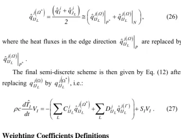
Using a local frame of reference, in which one axis is along the edge direction (P) and another axis (N) is in the plane orthogonal to direction (P), (see Fig. 1), the edge gradient can be alternatively computed as: j N IJ j P IJ j IJ x Tˆ x Tˆ x Tˆ L L L ∂ ∂ + ∂ ∂ = ∂ ∂ . (19)
Figure 1. Local frame of reference.
Once the nodal gradients are known the corresponding fluxes can be directly obtained by the use of the Fourier Constitutive Law given in Eq. (2), and, similarly to the edge values of the temperature gradients, the edge fluxes are given by:
( )
(
L)
( ) ( )L L L
j j I J
j j j
IJ IJ IJ
P N
ˆ ˆ
q q
ˆ ˆ ˆ
q q q
2
Ω = + =⎛ Ω + Ω ⎞
⎜ ⎟
⎝ ⎠ . (20)
Using a second-order central finite difference approximation, the temperature derivative over the edge in direction (P) can be calculated by: L L L * L IJ IJ I J P IJ X Tˆ Tˆ x Tˆ L ∆ − = ∂ ∂ . (21) Where L IJ
∆X is the size of the edge IJL, i.e.:
I J
IJL X L X
X = −
∆ with XI =
(
xI1,xI2,xI3)
, (22)L L L
IJ I J IJ
X
∆ X X L
L= = − and
L L
IJ j I j J j
X x x L
∆ −
= , (23)
where L represents the unitary vector defined in the edge direction from I to JL, and Lj are the director cosines.
The Cartesian components of the derivative on the edge direc-tion are given by,
* L *
L
p IJ j j P IJ
x Tˆ L x Tˆ
∂ ∂ = ∂ ∂
, (24)
and the Cartesian components of the portion of the gradient or-thogonal (or normal) to the edge direction is then,
L L L
N P
IJ IJ IJ
j j j
ˆ ˆ ˆ
T T T
x x x
∂ ∂ ∂
= −
∂ ∂ ∂ , (25)
where ∂TˆIJL ∂xK is calculated in a finite volume fashion given by
Eq. (18).
In short, the edge temperature gradient given by Eq. (19) is computed using the edge direction quantity calculated by Eq. (24) and the normal one using Eq. (25). Similarly, the edge fluxes com-ponents given by Eq. (20) are now replaced by Eq. (26), which is computed using the gradients as described previously and the Fou-rier Constitutive Law Eq. (2), i.e.,
( )
*(
)
( ) ( )L
L L * L
j j
j I J j j
IJ IJ IJ
P N
ˆ ˆ
q q
ˆ ˆ ˆ
q q q
2
Ω + ⎛ Ω Ω ⎞
= ≅⎜ + ⎟
⎝ ⎠, (26)
where the heat fluxes in the edge direction ( )
L
j IJ
P
ˆq Ω are replaced by
( ) L *
j IJ
P
ˆq Ω .
The final semi-discrete scheme is then given by Eq. (12) after
replacing IJj( )Ω
L
q by IJj
( )
Ω*L
q , i.e.:
( )
* ( )ˆ
ˆ ˆ
L L L L
j j
j j
I
I IJ IJ IJ IJ I I
L L
dT
c V C q D q S V
dt
Ω Γ
ρ = −⎛⎜⎜ + ⎞⎟⎟+
⎝
∑
∑
⎠ . (27)Weighting Coefficients Definitions
The definition of the weighting coefficients is presented here just for the two-dimensional model, which will be adopted for vali-dating the formulation and computational system developed. How-ever, similar definitions apply for the 3-D spatial model(Sorensen, 2001).
For two-dimensional problems, we have the mesh on a flat mid-dle plane defined by coordinates x1and x2.Then,Eq. (8) must first be integrated over x3 and then over a 2-D space. In such model, we have the nodal volume computed as VI =AIEI, where EI refers to the thickness of the domain at point I, and AI is the area of the con-trol volume surrounding node I. The 2-D weighting coefficients
j IJL
C and IJj
L
D are defined by
L
L
j j
K K IJ
K
j j
L L IJ
C A n
D A n
=
=
∑
, (28)where AK =LKEK with EK =
(
EI+EJL)
2 and LK is the length of each interface K associated to edge IJL. Each interface connects the element centroid (C) to the middle point (MP) of one of the edges that belongs to such element and AL=LLEL, where LL is half the size of the boundary edge under consideration and ELis defined similarly to EK.nKj and nLjare the outward normal direction co-sines to the interface K and L,respectively. The geometric parame-ters required for computing the weighting coefficients are detailed in Figs. 2 and 3.Figure 2. 2-D control volume and its geometric parameters.
Figure 3. 2-D boundary control volume and its geometric parameters.
Thermal Loads, Boundary Conditions and
Multi-Materials Domain
Thermal Loads
For the 2-D model, the thermal load S over the domain is repre-sented here as:
(
)
[
T T]
EQ
S= + αΩ a − , (29)
with
P C R
Q=Q +Q +Q , (30)
where the superscripts P, C, R accounts for thermal sources (or “sinks”) acting on a point, a curve or a region, respectively. On the right hand side of Eq. (29) the first term represents the thermal sources (or sinks) described in Eq. (30). The second term accounts for convection over each face of the two dimensional domain, αΩ
is the film coefficient where the subscript Ω is used to emphasize that it acts over the domain, while in Eq. (5), αΓ acts over the boundary with mixed boundary condition and E refers to the thick-ness of the domain. It should be observed that the second term does not exist in a three-dimensional model and the convection on the surface is accounted in the boundary conditions.
The integral of the thermal loads Q described by Eq. (30) is given by:
C R
P C R
Q d Q Q d Q d
Ω Γ Ω
Ω = + Γ + Ω
∫
∫
∫
. (31)In Equation (31), the term P P
Q Q d
Ω
=
∫
Ω considers the totalvalue of heat source for a unity volume and therefore QIP is just a point heat source computed at a given node I. If the point source is not applied at a nodal point its value is distributed to the nodes of the triangle that contains it, using a linear approximation (Lyra et al., 2000). The ADT (Alternate Digital Tree), (Bonet and Peraire, 1990), data structure and corresponding searching algorithm is used to determine the element that contains the position of the point load.
The flexibility of our two-dimensional mesh generator (Lyra and Carvalho, 2000) is exploited using the possibility to build a fictitious boundary along the curve where we want to apply a heat source. The term containing QC considers the heat source value for a strip of unity width over the plane and along the surface ΓC,
which represents the transversal section along the line heat source. Then, the boundary integral in (31) is easily approximated by each portion of the fictitious boundary associated to node I
( )
I
C
Γ as:
∑
∫
≅L L C I C
A Q d
Q
I C
Γ
Γ . (32)
The summation extends over the two edges connected to node I
that belong to the fictitious boundary and AL is an area computed as previously defined.
If the heat source per unit of volume QR is distributed over a re-gion ΩR, the third integral in Eq. (31) is then approximated in the
same fashion as the transient term given in Eq. (9), i.e. for each control volume surrounding node I,
I
R
I Ω ∈
∀ , we have:
I R I R
V Q d Q
I R
≅
∫
Ω
Ω . (33)
Finally, the convective type source term is computed for each node I,
I
R
I Ω ∈
∀ , by:
(
)
[
Ta T]
Ed R(
Ta TˆI)
VI EII R
R − ≅ −
∫
ΩΩ
Ω Ω α
α . (34)
For the previous loads given in Eqs. (33) and (34) a specific re-gion covering ΩR is built with the help of our mesh generator,
which allows for the generation of consistent multi-regions meshes. In Equation (34), for the explicit time integration adopted here, we can use the value of TˆI known from the previous time level.
Boundary Conditions
To compute the Dirichlet boundary condition, Eq. (3), it is enough to substitute TI by TI whenever required, i.e. ∀ I ∈ ΓD.
To impose the Neumann boundary condition, Eq. (4), the total boundary edge flux that appears in the boundary loop in Eq. (27) must be projected on the directions parallel and normal to the edge under consideration. The normal portion must then be replaced by the prescribed flux qn.
For Cauchy (or Robin) mixed boundary condition, Eq. (5), the value
(
− +qn αΓTa)
is known and computed in the same fashion as implemented to compute the Neumann boundary condition. The remaining term is computed for eachI
R
Γ according to:
RI
I L L
ˆ
Td T A
Γ Γ
Γ
α Γ ≅
∑
α∫
, (35)with
I
R
Γ being the portion of the ΓR boundary associated to node I
and the summation extends over the two boundary edges connected to node I. Following the procedure adopted in Eq (34), TˆIof Eq. (35) is taken as the temperature of node I obtained at the previous time level.
Multi-Materials Domain
Whenever addressing heat transfer problems which involve dif-ferent material properties on difdif-ferent portions of the domain we need to build proper meshes for each sub-region and to perform consistently the discretization of the governing equation in order to guarantee the correct solution through the interface of the sub-regions. As already mentioned, our mesh generator has the flexibil-ity to generate consistent meshes over multi-region domains.
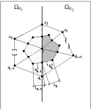
For each boundary and interior edges apart from the value of the weighting coefficients we identify and keep in memory the region that the edge belongs to, during the pre-processing stage. This is necessary to recovery the material properties used in the computa-tions during the processing stage. For each edge at the interface of two regions, the edge coefficient is computed independently for each region with the identification of the region also kept in mem-ory. Referring to Fig. 4, the edge IJL would have two coefficients defined by:
( ) and ( ) j k k R j IJ j
1 k 1 k R j
IJ A n C A n
C 2
L 1
Figure 4. Control volumes at an interface between two regions and their geometric parameters.
For the gradients and associated fluxes computations the proce-dure basically consists on three steps: first a loop over all edges of the mesh except the interface edges; second, a loop over the bound-ary edges and third, a double loop over the interface edges. In each of these loops we use the corresponding edge coefficients and asso-ciated material properties. In the computation of the “final” discrete equation, we can proceed similarly, with the corresponding proper-ties and thermal loads. The semi-discrete Eq. (27) is now replaced by:
( )
* ( ) 2 ( )( )
*1 ˆ
k
L L L L L L
j j j R j
j j
I IJ IJ IJ IJ IJ IJ I I
L L k L
dT
c V C q D q C q S V
dt
Ω Γ Γ
ρ
=
⎞ ⎛
⎟ ⎜
= −⎜ + + ⎟+
⎝
∑
∑
∑∑
⎠,
(37)
with the third term on the right hand side of Eq. (37) being non-zero only when node I is on the interface between two or more regions
( )
ΓI with different material properties. The external loop isneces-sary to consider twice each interface edges that are connected to
node I, i.e. once for each region. The interface edges fluxes
( )
* j IJ L
q Γ
are computed similarly to
( )
*L
j IJ
q Ω , see Eq. (26).
It should be observed that the proposed procedure is general, so that node I can belong to the interface of several regions, not just two and also that the interface does not need to be a straight line.
If the properties of the material, loads or boundary conditions vary in space, the middle point rule is adopted. For instance, the heat conductivity k of edge IJL is computed by:
2 k k
kIJL I J
+
= . (38)
If the material has non-linear behavior
[
e.g. k=f( )
T]
it is im-portant to use an iterative procedure, such as the Newton-Raphson method, but such feature has not yet been attempted in the present formulation.Some Important Numerical and Implementation Issues
In this section, several aspects referring to the generation and use of unstructured meshes, the adoption of an edge-based data structure and other related issues are addressed.
Unstructured Mesh Generation
In order to discretize arbitrary two-dimensional domains, we have developed a computational system(Lyra and Carvalho, 2000 and Carvalho, 2001) which can generate triangular, quadrilateral and mixed consistent meshes. The computational system deals with several connected domains and both isotropic and anisotropic meshes (i.e. directionally stretched meshes). In this work, only isotropic triangular meshes were considered and generated through the advancing front technique(Peraire et al., 1987), with the con-cepts of using a background grid to define the spacing, gradation and directionality of the mesh and of generating simultaneously points and triangles during the triangulation. As any conventional unstructured mesh generator the mesh data delivered consists of the physical coordinates simply listed by node numbers and a list of the connectivity of each element (topological information). Our mesh generator gives also a list of boundary edges connectivities, which are very helpful for the implementation of certain boundary condi-tions.
Edge-Based Data Structure and Its Implementation
A significant reduction in gather/scatter costs and memory re-quirements in the solver can be obtained by going from an element-based to an edge-element-based data structure (Lyra et al., 1998). This reduc-tionis more pronounced in three-dimensional simulations (Peraire et al., 1993). The adopted mesh generator, as any conventional un-structured mesh generator, provides the mesh data in an element-based data structure and the implementation of the finite volume solver described requires a pre-processing stage to convert the ele-ment-based data structure into edge-based. After the pre-processor stage is finished, the element-based data structure can be discarded.
The pre-processing stage consists basically on the following steps (Lyra, 1994):
1. Build the arrays with the mesh and boundary topology, which are lists of edges and boundary edges with their re-spective connectivities;
2. Compute and store the edge and boundary weighting coeffi-cients;
3. Transfer loads, material properties, boundary and initial conditions, which are associated to the geometry, to the mesh topological entities.
To extract the edges from the original data structure in an effi-cient way, a hash table searching technique is used (Lyra et al., 1998). The weighting coefficients are computed as described previ-ously. In our mesh generator all mesh topological entities (nodes, edges and elements) are associated to their correspondent geometric entity (point, curve or sub-domain). In this way, loads, material properties, boundary and initial conditions are initially associated to the geometry and then transferred to the topological data to get the finite volume model for the analysis. This is of particular impor-tance in an adaptive procedure as the mesh changes dynamically during the analysis and a new finite volume model has to be built for each new mesh.
contribu-tions to the nodes (or vertices) being accumulated during the proc-ess. The operations performed inside these loops, which take place in the edge-based solver algorithm are:
1. Gather Information the nodes of each edge; 2. Operate on this information;
3. Scatter the results back to the nodes of the edges and add them to the nodal quantities.
Numerical Results
In this section, some simple, though representative academic, examples are presented in order to validate and show some of the capabilities of the numerical scheme previously discussed. All steady-state solutions were obtained using the transient algorithm, which is stopped when the time derivative of the temperature is not changing, i.e. the residual is below a pre-assigned tolerance, with the adopted value of 10-7. For all steady-state solution we adopted the density ρ = 1.0 kg/m3 and the specific heat c = 1.0 J/kg K. These values guarantee that the equation is non-stiff and were not chosen taking into account any aspects related to computational efficiency. The results are post-processed using the scientific visualization tool “Mtool” (Tecgraf-PUC-Rio).
Steady-State Heat Conduction Problem
The first application refers to a steady state solution of a two-dimensional heat transfer problem in a rectangular plate of 0.6 m by 1.0 m and uniform unity thickness. The left face of the plate is insulated (zero heat flux), while the bottom edge is at a fixed tem-perature of 100 °C and the right and top edges are under convection to ambient temperature of 0 °C. The thermal conductivity of the plate is k = 52.0 W/m°C and the convective heat transfer coefficient is αΓ = 750.0 W/m2°C.
(a) (b)
Figure 5. 2-D heat conduction problem: (a) domain representation; (b) coarse mesh with 32 nodes.
The initial condition is an uniform temperature of Ti = 0.0 °C.
This example was extracted from the NAFEMS selected FE bench-marks in structural and thermal analysis (Barlow and Davies, 1987). Figure 5a shows the domain representation for this problem and Fig. 5b shows the triangular coarse mesh utilized. The target value to be achieved is a temperature of 18.3 °C in point E (see Fig. 5a).
In Table 1 we show the obtained results with two different uni-form meshes. The first one is a coarse mesh with 32 nodes, and the second one is a finer mesh with 793 nodes. It can be observed that the final results are in good agreement with the expected target value.
Table 1. Temperatures at node (E) obtained with two different mesh densi-ties.
TEMPERATURE AT NODE E (0C)
NAFEMS Coarser Mesh Finer Mesh
18.30 18.14 18.29
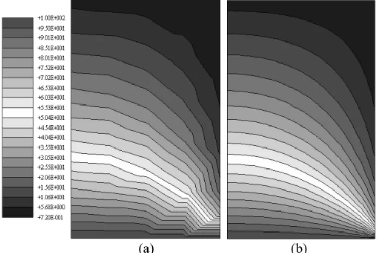
Figure 6 shows the contours of temperature for both meshes. It is important to note that even the coarse mesh provided a good result if compared with the NAFEMS results. As expected, for the finer mesh, the contours of temperature are much smoother than those obtained with the coarser one. Only uniform meshes have been used up to now, but the results can certainly be much better, even for meshes with the size of the coarse mesh, if the knowledge of the expected solution is used to build the mesh or an automatic error analysis and adaptive procedure is incorporated (Lyra et al., 2000).
(a) (b)
Figure 6. 2-D heat conduction problem. Temperature contours: (a) For the coarser mesh (32 nodes); (b) For the finer mesh (793 nodes).
Multi-Material Steady-State Heat Conduction Problem
In the second example, we present a steady state problem of a rectangular plate of unity thickness compounded by two materials with different conductivities. The 2-D domain representing the plate was subdivided into two sub-domains where the triangular mesh was built independently for each sub-domain (representing each material), keeping the consistency of the mesh between them. First we analyze the plate with an interface between the materials which is placed in the middle of the plate and it is perpendicular to its base as shown in Fig. 7. Then we analyze a plate in which the interface between the two materials is semicircular as shown in Fig. 8.
Figure 8. Domain for multi-material heat conduction problem with a semi-circular interface between both materials.
In both cases, with perpendicular and curvilinear interfaces, the plate is subjected to a prescribed temperature (T = 100 °C) on its left side and, the top and the bottom sides of the plate are insulated. On the right side, the plate is under convection, with the convection heat transfer coefficient αΓ = 100.0 W/m2°C and the ambient temperature of Ta = 30 0C. The thermal conductivity of the left and right parts of the plate are, respectively, kL = 50.0 W/m°C, kR = 15.0 W/m°C. The initial condition considered is a uniform temperature of Ti = 30 °C.
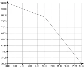
For the first case (with a perpendicular interface between the two materials), a uniform triangulation with 216 nodes and 410 elements was adopted. Figures 9 and 10 show, respectively, the contours of temperature for this problem, and the temperature distri-bution for y = 0.0 and 0.0 ≤x≤ 20.0. In Figure 10, we can note the abrupt change in the slope of the temperature distribution due to the change in the conductivity coefficient of the two adjacent materials. In Table 2 we can see the good agreement achieved when we com-pare the nodal temperatures at the right side and at the interface between the two different materials, with the 1-D analytical solu-tion.
Figure 9. Temperature contours for multi-material heat conduction prob-lem.
Figure 10. Temperature distribution over the y = 0.0 axes for 0.0 ≤ x ≤ 20.0, for the multi-material heat conduction problem with a perpendicular interface.
Table 2. Nodal temperatures at the right side and at the perpendicular interface between the two different materials.
x (m) Analytical Solut. (0C) Numerical Solut. (0C)
10 84.03 84.04
20 30.79 30.79
Figure 11 shows the heat flux vectors and the isolines of tem-perature for the case with a semicircular interface between the two materials. In this figure we can readily verify the small value of the
y component of the fluxes at the interface and the essentially 1-D behavior of the heat transfer when the distance from the interface increases. For this analysis a uniform triangular mesh with 303 nodes and 534 elements was used.
Figure 11. Triangular mesh and heat flux vectors for the multi-material heat conduction problem with a semi-circular interface.
In this latter case, the energy conservation (integral of the fluxes) was checked. For this purpose we computed the integral of the fluxes at the inflow (left) and outflow (right) faces of the plate, and the relative difference obtained was of 0.53% between the two faces.
Transient Heat Transfer Through an Infinite Slab
In the final example, we show a transient one dimensional heat transfer problem in which the domain is represented by an infinite slab of unit thickness with length L in the x direction and of “infi-nite” length in the y direction. The slab is initially at a temperature of i
W/m3 is applied over the entire domain. The thermal conductivity of the medium is k = 34.61 W/m°C, its density is ρ = 8009.25 kg/m3, and its specific heat is c = 8373.34 J/kg°C. The surfaces in x= 0 e x = L are kept at a temperature TS = 0 °C. Figure 12 shows a sketch of the domain for this problem.
Figure 12. Slab of length x = L and “infinite” length in the y direction subjected to a uniform distributed heat source Q.
In order to represent the infinite slab and after some numerical experimentation we use a computational domain with 2L length in the y direction. Due to the symmetry of the problem we simulate only a quarter of the slab. On the two symmetry axis (right vertical and lower horizontal faces of the computational domain) an adia-batic flux condition (qn = 0.0 W/m2) is prescribed. On the left verti-cal face the prescribed temperature is TS = 0 °C. Finally, on the upper horizontal face, which represents the surface of the domain truncated for numerical purposes, we also set a prescribed flux qn = 0.0 W/m2. The triangular mesh used in the simulation has 72 nodes and 112 elements. Figure 13 shows the mesh and the contours of temperature at instant t = 720 sec.
(a) (b)
Figure 13. Infinite slab problem at t = 720 sec.: (a) Contours of temperature; (b) Triangular mesh.
In order to verify the accuracy of our results, we compared them to the solution obtained with the commercial software “ANSYS”, with a similar mesh density, and we also compared our results with the analytical solution obtained using up to three terms of the infi-nite series solution given in ANSYS verification manual (see AN-SYS Internet address).
Tables 3 and 4 show, respectively, the temperatures and the tem-peratures ratios, obtained dividing ANSYS and finite volume solu-tions by the analytic one, i.e. (ANSYS/Analytic.) and (FVM/Analytic.). The results were obtained at time t = 720 sec, for the collinear nodes 3, 4, 5, 6 and 2 localized at the left bottom side of Fig. 13b. As it can be observed, the results obtained with the FVM show very good agreement with the analytical solution and a comparable performance to that obtained with the finite element method (FEM) attained using the ANSYS software.
Table 3. Temperatures at five collinear nodes, obtained through different methods: Analytic, FEM (ANSYS), Finite Volume (FVM).
Temperature (0C) at time t =720 s
Nodes Analytic. ANSYS FVM
3 24.31 24.10 23.76
4 40.00 39.60 39.36
5 49.33 48.77 49.06
6 54.14 53.48 53.86
2 55.61 54.92 54.95
Table 4. Temperature ratios at five collinear nodes between AN-SYS/Analytical and FVM/Analytical solutions.
Temperature ratios at time t =720 s
Nodes ANSYS/Analytic. FVM/Analytic.
3 0.991 0.977 4 0.990 0.984 5 0.988 0.994 6 0.988 0.995 2 0.988 0.988
Concluding Remarks
Acknowledgements
The authors would like to acknowledge the Brazilian Research Council CNPq and the National Petroleum Agency (ANP) for the financial support provided during the development of this research.
References
AGARD Report 787, 1992, “Special Course on Unstructured Grid Methods for Advection Dominated Flows”, France.
ANSYS Verification Manual. Internet Adress: http www1.ansys.com/customer/content/documentation/60/Hlp_V_VMTOC.html
Barlow, J. and Davies, G.A.O., 1987, “Selected FE Benchmarks in Structural and Thermal Analysis”, NAFEMS (National Agency for Finite Element Methods & Standards), National Engineering Laboratory, Glasgow, U. K.
Barth, T.J., 1992, “Aspects of Unstructured Grids and Finite-Volume Solvers for the Euler and Navier-Stokes Equations”, AGARD Report 787, pp. 6.1-6.61.
Bonet, J. and Peraire, J., 1990, “An Alternating Digital Tree (ADT) Al-gorithm for 3-D Geometric Searching and Intersection Problems”, Interna-tional Journal for Numerical Methods in Engineering, Vol. 31, pp.1-17.
Carvalho, D.K.E., 2001, “A Computational System for the Generation and Adaptation of Bidimensional Unstructured Meshes”. Master Disserta-tion, Department of Mechanical Engineering, Federal University of Pernam-buco, Brazil, DEMEC-UFPE, (In Portuguese).
Crumpton, P.I., Moinier, P. and Giles, M.B.T.J., 1997, “An Unstruc-tured Algorithm for High Reynolds Number Flows on Highly Stretched Grids”. In: C. Taylor and J. T. Cross, (editors), Numerical Methods In: Laminar and Turbulent Flow, Pineridge Press, pp.561-572.
Guimarães, C.S.C., 2003, “Computational Modeling of the Bioheat Transfer During the Hyperthermic Treatment of Duodenum Tumors Using an Unstructured Mesh Finite Volume Method”. Master Dissertation, Me-chanical Engineering, DEMEC-UFPE, (In Portuguese).
Lima, R. de C.F. de, Lyra, P.R.M. and Guimarães, C.S.C., 2002, “A Technique to Compute Temperatures in Abdominals Tumors by the Solution of the Bioheat Transfer Equation Through the Use of The Finite Volume Method on Unstructured Meshes”, LATCYM2002 – Nono Congreso Latino Americano de Transferencia de Calor y Materia, Porto Rico, november, pp. 1-13, in CD-ROM (In Portuguese).
Lyra, P.R.M., 1994, “Unstructured Grid Adaptive Algorithms for Fluid Dynamics and HeatConduction”, Ph.D. thesis C/PH/182/94, University of Wales - Swansea.
Lyra, P.R.M., Morgan, K., Peraire, J. and Peiró, J., 1994, “TVD Algo-rithms for the Solution of the Compressible Euler Equations on Unstructured Meshes”, International Journal for Numerical Methods in Fluids, Vol. 19, pp. 827-847.
Lyra, P.R.M., Willmersdorf, R.B., Martins, M.A.D. and Coutinho, A.L.G.A., 1998, “Parallel Implementation of Edge-Based Finite Element Schemes for Compressible Flows on Unstructured Grids”, VECPAR’98 – Third International Meeting on Vector and Parallel Processing, Porto, Portu-gal, pp. 99-111.
Lyra, P.R.M and Carvalho, D.K.E., 2000, “A Flexible Unstructured Mesh Generator for Transient Anisotropic Remeshing”, ECCOMAS 2000 – European Congress on Comp. Meth. in Applied Sciences and Eng., Barce-lona-Espanha, september, published in CD-ROM.
Lyra, P.R.M, Almeida, F.P.C., Willmersdorf, R. B., and Afonso, S.M.B., 2000, “An Adaptive FEM Integrated System for the Solution of Transient Thermal-Structural Problems”, CILAMCE 2000 - Iberian Latin American Congress on Computational Methods in Engineering, Rio de Janeiro-Brasil, december, pp. 1-18, published in CD-ROM.
Lyra, P.R.M., Lima, R.C.F., Guimarães, C.S.C. and De Carvalho, D.K.E., 2002, “An Edge-Based Unstructured Finite Volume Method for the Solution of Potential Problems”, MECOM'2002 - First South American Congress on Computacional Mechanics, Parana and Santa Fé, Argentina, November, 2002, pp. 1-19, published in CD-ROM;
Peraire, J., Vahdati, M., Morgan, K. and Zienkiewicz, O.C., 1987, “Adaptive Remeshing forCompressible Flow Computations”, Journal of Computational Physics,Vol. 72, pp. 449-66.
Peraire, J., Peiró, J. and Morgan, K., 1993, “Finite Element Multigrid Solution of Euler Flows Past Installed Aero-Engines”, V.11.433-451, J. Computational Mechanics.
Sorensen, K.A., Hassan, O., Morgan, K. and Weatherill, N. P., 1999, “An Aglomeration Unstructured Hybrid Mesh Method for 2D Turbulent Compressible Flows”, ISCFD’99,Bremen, published in CD-ROM.
Sorensen, K.A., 2001, “A Multigrid Procedure for the Solution of Com-pressible Fluid Flows on Unstructured Hybrid Meshes”, Ph.D. thesis C/PH/251/01, University of Wales - Swansea.
Sorensen, K.A., Hassan, O., Morgan, K. and Weatherill, N., 2001, “Ag-glomeration Multigrid on Hybrid Meshes for Compressible Viscous Flows”, ECCOMAS European Computational Fluid Dynamics Conference, pub-lished in CD-ROM.