Generating Time Optimal Trajectory
from Predefined 4D waypoint Networks
Kawser Ahmed, Kouamana Bousson
Abstract
– The main purpose of this paper is to develop a trajectory optimization method to generate optimal trajectories that minimize aircraft total trip time between the initial and final waypoint in predefined 4D waypoint networks. In this paper, the 4D waypoint networks only consist of waypoints for climb, cruise and descent approach without the take-off and landing approach phases. The time optimal trajectory is generated for three different lengths of flights (short, medium, and long-haul flight) for two different commercial aircraft and considering zero wind condition. The Results about the presented applications show that by flying a time optimal trajectory, which was found by applying a single source shortest path algorithm (Dijkstra’s algorithm), can lead to the reduction of average travel time by 2.6% with respect to the total trip time. Copyright © 2017 Praise Worthy Prize S.r.l. - All rights reserved.Keywords:
Time Conservation, Cost Index, 4D Waypoint Navigation, Trajectory Optimization, Dijkstra’s Algorithm, Base of Aircraft Data (BADA)Nomenclature
a Acceleration
a Earth semi major axis
L
C Lift coefficient
d Travel time between waypoints
e Eccentricity
G,w,s Graph, weight, and source vertex
P Waypoint
e
R Earth radius
S Wing area
V Flight velocity
V,E Vertices and edge of the graph TAS
V True air speed
W Aircraft Nominal weight X ,Y ,Z Geocentric Coordinates
, ,h
Longitude, Latitude, and altitude
Arrival time tolerance interval
Flight path angle
Air density
Arrival time at waypoint
Heading
d
Distance between waypoints
I.
Introduction
The air traffic load on the European air traffic network grows year upon year, the volume of air traffic is expected to double over the next 20 years.
Hence developing optimal trajectory that minimizes travel time on flight mission for commercial aircraft becomes an important factor nowadays not only because it helps the airlines to reduce their time related operating
costs but also as it enhances air traffic flow in this rapidly growing aviation industry.
A practical solution that reduces the cost associated with time and fuel consumption during flight is the Cost Index (CI). The value of the CI reflects the relative effects of fuel cost on overall trip cost as compared to time-related direct operating cost. For all the aircraft models, the minimum value of cost index equal to zero results in maximum range airspeed and minimum trip fuel, but this configuration ignores the time cost. If the cost index is maximum, the flight time is minimum, the velocity and the Mach number are maximum, but ignores the fuel cost [1]. In this paper, the Cost Index assumes to be maximum as only time cost is taken into consideration. The cost index is shown in equation (1):
€/hour €/kg TimeCost ~ CI FuelCost ~ (1)Trajectory optimization is a vital area in aeronautic industry. This technique enables generating optimal trajectories for vehicles with consideration of fuel consumption, travel time and many other requirements. The trajectory optimization problem can be solved by optimal control methods. The optimal control problem can be solved by various kind of methods, however, these methods can be separated into two basic approaches: the indirect approach and the direct approach [2], [3].
The optimal control is solved by the Pontryagin maximum principle [4] in indirect approach, where the original optimal control problem is converted into Euler-Lagrange system (boundary value problem) by formulating the first order necessary condition which
derived from Pontryagin maximum principle. Generally, the indirect approach leads to more accurate results than the direct approach. However, in indirect approach a good initial approximation of the co-state equation is needed in order to convergence, the physical meaning of co-state equation is not well established which make it difficult to guess [5]. Solving the optimal control problem by indirect approach also leads to two-point boundary value problem (TPBVPs), it demands computationally intensive iterative numerical procedures. The direct approach is based on the transformation of optimal control problem into parameter optimization problem [6]. Which is done by discretizing the infinite dimensional problem into a finite dimensional problem and later on solving it by the nonlinear programming. Direct methods tend to have better convergence properties over indirect methods. Another great advantage of direct methods is that they do not have to deal with co-state equation. The most known direct approaches are based on Runge-Kutta scheme [7] and collocation methods [8]. Recently, some works have been presented for higher nonlinear dynamic system called a Chebyshev pseudo-spectral method [9], [10], [11].
Some research activities have been done for optimal trajectory generation in pre-defined network. Recently Boukraa, Bestaoui and Azouz [12] propose 3D optimal trim trajectories planner algorithm to generate trajectories for a set of predefined waypoints in space. However, the arrival time of each of these waypoints is not specified in their trajectory model. Bousson and Gameiro [13] present a quintic spline approach for 4D trajectory generation for UAVs. Devika and Thomas [14] present a path planning algorithm based on linear programming is adopted to ensure conflict free path in minimum time.
In this present paper, we suggest a new approach to generate 4D optimal trajectory defined by waypoints. In 4D trajectory the waypoints are consist of tri-dimensional coordinates as well as the arrival time in each waypoint. In this approach, the optimal trajectory is generated by applying greedy shortest path algorithms in graph theory, where the 4D waypoint networks are already pre-specified. The shortest path algorithm approximates an optimal trajectory by the path that minimizes the total link cost connecting the origin and destination in a pre-defined network. This approach often require large computation time and memory space as the network grows bigger but the global optimal solutions is guaranteed to be found. In this paper, the single source shortest path algorithm (Dijkstra’s algorithm) is used to generate the time optimal trajectory.
This study is restricted to the climb, cruise and descent phases of the flight and ignores the take-off and landing approach, and assuming the initial and final waypoints are at altitude of 3000 feet, where in the initial waypoint the aircraft begins the climb phase and in the final waypoint the aircraft begins the landing approach.
This paper primarily attempts to quantify benefits of time optimal trajectory which was generated by implying
the Dijkstra’s shortest path algorithm, here a benefit is meant to imply a reduction in total travel time due to using the Dijkstra’s shortest path algorithm to the actual unimproved flight. The key aspect of this paper is a detailed comparison between actual flight trajectories and corresponding more efficient trajectory, thus giving the most realistic estimate of improvement potential.
II.
Problem Statement
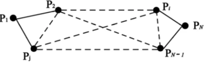
The main goal of this paper is to find a time optimal path from predefined 4D waypoint networks. A representation of waypoint networks is shown in Fig. 1, where P is the initial waypoint and 1 P is the final N waypoint of the networks.
Fig. 1. Representation of 4D waypoint networks
Most of the approaches consider the waypoints defined by tri-dimensional coordinates positions as:
Tk k k k
P , ,h , where k1 2, ,...,i, j,..., N and do not take into account the arrival time k at that waypoint. By adding the arrival time restriction, it is possible to define the 4D waypoints as: Pk
k, k,h ,kk
T. Where:k, k,h ,k k
is respectively longitude, latitude, altitude, and arrival time at waypoint P . k
The problem to be solved is to estimate associated travel time dk between the waypoints in 4D waypoint networks, then to use the value of associated travel time
k
d between pair of waypoints as edges E and the waypoints as vertices V in Dijkstra’s single source shortest path algorithm to generate the time optimal trajectory between the initial and final waypoints from the networks.
The following section propose a method that will generate the time optimal path along specified waypoints from predefined 4D waypoint networks by implying the Dijkstra’s single source shortest path algorithm.
III. Proposed Method
To generate an optimal trajectory which minimizes travel time between the initial and final waypoints from a set of waypoints in 4D waypoint networks requires finding the associated travel time dk by the aircraft to go from one waypoint to the other, defined as:
1
k k k
where, dk [min] is the travel time needed to go from waypoints Pk1 toP , k k[min] is the travel time required to get to waypoint P from initial waypoint and k k1
[min] is the travel time required to get to waypoint
1 k
P from initial waypoint.
In practice, the aircraft may not pass through the waypoint P exactly at the specified time k k due to disturbances that may give rise to navigation inaccuracies. Therefore, an appropriate way is rather imposing a time tolerance interval
at each waypoint:1
k k d k
(3)
where, is the time tolerance interval for arrival at a determined waypoint
11 4.
. In the case when both waypoints Pk1 and P are at same altitude, the time k tolerance interval can be assumed as 1.III.1. Dijkstra’s Algorithm
Dijkstra's algorithm, was first proposed by Dutch computer scientist Edsger Dijkstra in 1956 and published in 1959, is the most well-known shortest path algorithm. This is a graph search algorithm that solves the single-source shortest path problem for a graph with non-negative edge path costs, producing a shortest path tree. The most common variant of the algorithm fixes one vertex as the source and another as the destination vertex and find the shortest path between them.
Dijkstra’s algorithm solves the single-source shortest-paths problem on a weighted, directed graph G (V, E) where V is a set of vertices and E is a set of edges on the graph. This algorithm requires 3 variables as input in order to finds the path with lowest cost between the source and destination vertices, they are respectively the graph, the source vertex, and the destination vertex, and at the end it returns a reduced graph as output.
This algorithm will determine the global optimal (best route to take), given a number of vertices and edges as long as it has the graph as an input, no matter how large the graph is.
In addition to the basic formulation of the Dijkstra’s algorithm, the following aspects must be defined specifically for the flight trajectory optimization problem. The number of vertices V, the edges E between the vertices and the source and destination vertices. In this paper, the waypoints of the 4D waypoint networks are the vertices V, the initial waypoint is the source vertex s, the final waypoint is the destination vertex and the associated travel time dk by the aircraft between the pairs of waypoints are the edges E between these vertices (waypoints).
In Figs. 2 a full execution of the Dijkstra’s shortest path algorithm operation is shown. The circles represent the vertices or nodes and the lines with arrows are the edges.
Figs. 2. The execution of Dijkstra's algorithm
Each edge has a non-negative cost associated with it. The problem is to find the most cost-efficient route from the source vertex to any other vertex.
In this example, the source vertex s is the leftmost vertex. The value with low cost estimates appear within the vertices, and shaded edges indicate predecessor values. Black vertices are already examined thus they have the value of lowest cost associated with them to go from the source vertex, and the white vertices are going to be examined. First step (a) shows the situation just before the first iteration of the while loop. Form step (b) to step (f) shows the situation after each successive iteration of the while loop. The value of lowest cost and predecessors shown in last step (f), and these are the final values of the lowest cost to go to that vertex from the source vertex [15], [16], [17].
III.2. Modelling of 4D Waypoint Network Assuming the 4D waypoint networks consists of N sets of waypoints, where P is the initial waypoint and 1
N
P is the final waypoint in the waypoint networks. Each waypointP , where k k1 2, ,...,i, j,..., N is defined by the geodetic coordinates k, k,hk, by considering the arrival time in each waypoint, the waypoint P can be k described as a four-dimensional state vector:
Tk k k k k
P , ,h , (4)
where, k is the longitude, k is the latitude, h is the k altitude (with respect to sea level) and k is the scheduled arrival time at waypoint P . The following k subsections represent the navigation model and constraints of 4D waypoint networks.
III.2.1. Navigation Model
The following differential equations model the dynamics of the navigation process:
e
V cos sin R h cos (5)
e
V cos cos R h (6) hV sin (7) 1 Vu (8) 2 u (9) 3 u (10)where, V is the flight velocity, is the flight path angle,
is the heading (with respect to the geographical north), is the longitude, is the latitude, h is the altitude (with respect to sea level) and R is the Earth e radius.
The variables u , 1 u and 2 u are respectively the 3 acceleration, the flight path angle rate, and the heading rate. The state vector x and control vector u of the above model are described respectively as:
Tx , ,h,V , , (11)
1 2 3
Tu u u ,u, (12)
III.2.2. Navigation Constraints
The real-world flight operates under several constraints, due to aircraft performance, aerodynamic, structural limits, safety reasons, the mission and other factor, which is described as:
min max a a a (13) min max (14) min max V V V (15)
These bound constraints are imposed on the state and control vectors.
III.3. Arrival Time at Each Waypoint
The 4D navigation consists of traveling through a sequence of predefined waypoints in a given time of flight, which in turn define the trajectory of the flight. Assuming that the waypoint P is already defined by the k geodetic coordinates longitude k, latitude k, and altitude h , where the scheduled time of arrival k k at this waypoint is unknown. To compute this unknown arrival time of each waypoint, the distance between this waypoint and its previous waypoint from where the
aircraft is arriving and the average velocity of the aircraft between these two waypoints are required.
The trajectory generation requires a geocentric coordinates system. To calculate the distance between two waypoints, the tri-dimensional waypoints need to be transformed from usual geodetic coordinates system to geocentric coordinates system. The 3D waypoint P is k defined by the following way:
Tk k k k
P , ,h (16)
Now to transform these geodetic coordinates to geocentric coordinates, the following equations are required [18]:
k k k k k X N h cos cos (17)
k k k k k Y N h cos sin (18)
2
1 k k k k Z N e h sin (19)Being a is the Earth semi major axis and e its eccentricity, N can be calculated as follows: k
2 2 a 1 k k N e sin (20)
After transforming the 3D waypoints from geodetic coordinates to geocentric coordinates system, now it is possible to calculate dk (the distance between two waypoints Pk1 and P ) by using the following equation: k
1
2
1
2
1
2k k k k k k k
d X X Y Y Z Z
(21)
To estimate the appropriate velocity of the aircraft V k at any waypoint P , the following equation can be used: k
2 k k L W V C S (22)
where, W is the aircraft nominal weight, C is the lift L coefficient, S is the wing area of the aircraft and k is the air density (varies with altitude) at waypoint P . It is k possible to get the appropriate velocity at any waypoint
k
P from Base of Aircraft Data (BADA), where true air speed, VTAS [kt] is specified for different aircraft for different flight level and phases of the flights [19].
By using the distance between two waypoints and the velocity of the aircraft in both waypoints the travel time between these two waypoints can be computed as follow:
1 2 k k k k d d V V (23)
where, dkis the time needed to go from waypoint Pk1 to P . k
IV. Simulation and Result
In this section, the simulation and result of the time optimal trajectory is shown for three different length (short, medium, and long-haul) of flight considering zero wind conditions. All the analysis of the simulation has been done using Matlab 2013a. The coordinates of the trajectory were chosen using sky vector website [20].
IV.1. Short-Haul Flight
In order to analyze the short-haul flight, the flight from Lisbon to Geneva was considered. The 4D waypoint networks of this short-haul flight consists of two different trajectories, and has total 22 waypoints including the initial and final waypoints, and each trajectory has 12 waypoints including the initial and final waypoints. Airplane A1 (which is a short to medium range narrow body twinjet airliner) was used to analyze the flight trajectories. Tables I and II show the waypoints lists for both of the trajectories. Each waypoint is defined in geodetic coordinates
, , h
, and their associated distance travel time dk between the waypoints are also shown.The trajectories were chosen such a way that the climb and descent phases of the first trajectory are smaller than the second trajectory but the cruise phase of the first trajectory is bigger than the second trajectory, therefore the total distance from the initial to final waypoint for both of the trajectories are more or less same. The time optimal trajectory was generated from the 4D waypoint networks by using the Dijkstra’s single source shortest path algorithm.
TABLEI
LIST OF WAYPOINTS IN 1ST TRAJECTORY FOR SHORT-HAUL FLIGHT
waypoint [deg] [deg] h [feet] k d [min] Initial (P1) -9.0405 38.9955 3000 0 P2 -8.9083 39.1087 10000 2.371751 P3 -8.624 39.33417 20000 3.437191 P4 -7.7987 39.8783 33000 7.295251 P5 -6.9993 40.2513 39000 5.748997 P6 -3.3707 43.227 39000 32.48854 P7 0.1303 44.729 39000 23.71969 waypoint [deg] [deg] h [feet] k d [min] P8 3.5963 44.9543 39000 19.97808 P9 3.87217 45.1205 33000 2.058735 P10 4.6985 45.41983 20000 5.71202 P11 5.336 45.606 10000 5.275779 Final (P22) 5.7553 45.884 3000 5.618537 Total 113.7046 TABLEII
LIST OF WAYPOINTS IN 2ND TRAJECTORY FOR SHORT-HAUL FLIGHT
waypoint [deg] [deg] h [feet] k d [min] Initial (P1) -9.0405 38.9955 3000 0 P12 -8.835 39.0883 10000 2.862798 P13 -8.49983 39.30183 20000 3.66612 P14 -7.59217 39.7763 33000 7.374258 P15 -6.715 40.11317 39000 6.036433 P16 -1.765 41.631 39000 32.6647 P17 0.5565 43.9993 39000 23.55432 P18 3.6277 44.85317 39000 19.04446 P19 3.9993 44.9983 33000 2.415762 P20 4.8617 45.261 20000 5.787862 P21 5.4975 45.5203 10000 5.625951 Final (P22) 5.7553 45.884 3000 5.642634 Total 114.6753
The time optimal trajectory contains 10 waypoints [initial waypoint (P1) → P2→ P3→ P4→ P5→ P8→ P9→ P10→ P11→ final waypoint (P22)], the distance between the initial and final waypoints in the time optimal trajectory is 777.8 nm. The comparison of travel time in different phases of flight for those two trajectories and time optimal trajectory is shown in (Table III).
TABLEIII
TOTAL TIME NEEDED IN DIFFERENT TRAJECTORIES
FOR SHORT-HAUL FLIGHT
Trajectory Time [min] Total
[min] Climb Cruise Descent
1 18.9 76.2 18.7 113.7
2 19.9 75.3 19.5 114.7
Time optimal 18.9 73.49 18.7 111.01
As it is seen from Table III that by using the time optimal trajectory in short-haul flight (Lisbon – Geneva), the aircraft reaches the final waypoint 2.7 minutes faster than the first trajectory, which is equivalent to 2.4% of total travel time of the first trajectory and 3.7 minutes faster than the second trajectory equivalent to 3.2% of total travel time of the second trajectory. The time optimal trajectory of short-haul flight is shown in Fig. 3.
In Fig. 3 the blue curve line represents the real trajectory path through different waypoints, starting on the right. The red circles around the blue line denote the position of the waypoints associated with the trajectory.
Fig. 3. 3D time optimal trajectory in geocentric coordinates for short-haul flight
IV.2. Medium-Haul Flight
To analyze the medium-haul flight, the flight from Lisbon to Stockholm was considered.
There are also two trajectories between the initial and final waypoints in the 4D waypoint networks, each trajectory has total 13 waypoints including the initial and final waypoints, and total 24 waypoints are there in the 4D networks including the initial and final waypoint. Airplane A2 (which is a long range wide body twinjet airliner) was used to analyze the flight trajectories.
Tables IV and V show the waypoints lists for both trajectories.
TABLEIV
LIST OF WAYPOINTS IN 1ST TRAJECTORY
FOR THE MEDIUM-HAUL FLIGHT
waypoint [deg] [deg] h [feet] k d [min] Initial (P1) -9.0405 38.9955 3000 0 P2 -8.9373 39.1525 10000 2.665515 P3 -8.643 39.6385 24000 5.529098 P4 -8.0007 40.5407 37000 8.291856 P5 -7.7847 40.942 41000 3.243938 P6 -4.752 46.1707 41000 42.43539 P7 1.07817 49.6497 41000 39.21055 P8 9.07617 53.515 41000 47.18143 P9 14.4575 57.839 41000 39.59531 P10 14.75417 58.0005 37000 1.695762 P11 15.78983 58.624 24000 6.807662 P12 17.0113 59.2063 10000 9.043191 Final (P24) 17.73983 59.3445 3000 5.538229 Total 211.2379 TABLEV
LIST OF WAYPOINTS IN 2ND TRAJECTORY
FOR THE MEDIUM-HAUL FLIGHT
waypoint [deg] [deg] h [feet] k d [min] Initial (P1) -9.0405 38.9955 3000 0 P13 -8.8405 39.1047 10000 2.874146 P14 -8.455 39.576 24000 5.748028 P15 -7.808 40.4545 37000 8.141368 P16 -7.413 40.8377 41000 3.642769 P17 -0.2773 44.76 41000 49.00066 waypoint [deg] [deg] h [feet] k d [min] P18 4.6187 50.023 41000 46.56667 P19 10.92483 54.85883 41000 46.27695 P20 15.0405 57.2845 41000 25.06379 P21 15.39 57.4757 37000 2.016462 P22 16.496 58.17 24000 7.488843 P23 17.504 58.94117 10000 9.827318 Final (P24) 17.73983 59.3445 3000 5.864875 Total 212.5119
The time optimal trajectory for the flight between Lisbon and Stockholm (medium-haul flight) contains 9 waypoints [initial waypoint (P1) → P2→ P3→ P4→ P5→ P9→ P10→ P12→ final waypoint (P24)], the distance between the initial and final waypoints in time optimal trajectory is 1589.6 nm.
The comparison of travel time in different phases of the flight for those two trajectories and the time optimal trajectory is shown in Table VI.
It can be seen from Table VI that by flying the time optimal trajectory in medium-haul flight (Lisbon – Stockholm) 4.2 minutes can be saved than the first trajectory, which is equivalent to 1.9% of total travel time of the first trajectory and 5.5 minutes can be saved
than the second trajectory, which is equivalent to 2.6% of total travel time of the second trajectory. The time optimal trajectory is shown in Fig. 4.
In Fig. 4 the blue curved line is the time optimal trajectory path and the red circles around it are the associated waypoints of the time optimal trajectory.
TABLEVI
TOTAL TIME NEEDED IN DIFFERENT TRAJECTORIES
FOR MEDIUM-HAUL FLIGHT
Trajectory Time [min] [min] Total Climb Cruise Descent
1 19.7 168.4 23.1 211.2
2 20.4 166.9 25.2 212.5
Time optimal 19.7 164.3 23.04 207.04
Fig. 4. 3D time optimal trajectory in geocentric coordinates for medium-haul flight
IV.3. Long-Haul Flight
The flight from Lisbon to Montreal was considered in order to analyze the long-haul flight.
The 4D waypoint networks of the long-haul flight also consists of two trajectories between the initial and final waypoints, each trajectory has 14 waypoints including the initial and final waypoints, and total 26 waypoints are in the whole 4D waypoint networks including initial and final waypoints.
Airplane A2 (which is a long range wide body twinjet airliner) was used to analyze the flight trajectories. The waypoints list of both trajectories is shown in Table VII and VIII.
TABLEVII
LIST OF WAYPOINTS IN 1ST TRAJECTORY
FOR THE LONG-HAUL FLIGHT
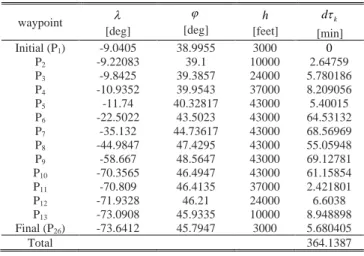
waypoint [deg] [deg] h [feet] k d [min] Initial (P1) -9.0405 38.9955 3000 0 P2 -9.22083 39.1 10000 2.64759 P3 -9.8425 39.3857 24000 5.780186 P4 -10.9352 39.9543 37000 8.209056 P5 -11.74 40.32817 43000 5.40015 P6 -22.5022 43.5023 43000 64.53132 P7 -35.132 44.73617 43000 68.56969 P8 -44.9847 47.4295 43000 55.05948 P9 -58.667 48.5647 43000 69.12781 P10 -70.3565 46.4947 43000 61.15854 P11 -70.809 46.4135 37000 2.421801 P12 -71.9328 46.21 24000 6.6038 P13 -73.0908 45.9335 10000 8.948898 Final (P26) -73.6412 45.7947 3000 5.680405 Total 364.1387
TABLEVIII
LIST OF WAYPOINTS IN 2ND TRAJECTORY
FOR THE LONG-HAUL FLIGHT
waypoint [deg] [deg] h [feet] k d [min] Initial (P1) -9.0405 38.9955 3000 0 P14 -9.2387 39.05683 10000 2.514717 P15 -9.94583 39.2603 24000 6.040968 P16 -11.2588 39.4515 37000 8.362034 P17 -11.9673 39.9493 43000 5.533107 P18 -24.8818 42.095 43000 74.7246 P19 -34.374 43.996 43000 53.92886 P20 -44.3497 46.44083 43000 55.77103 P21 -61.77 47.44 43000 89.28184 P22 -70.163 46.2543 43000 43.99628 P23 -70.557 46.102 37000 2.317716 P24 -71.739 45.9043 24000 6.98395 P25 -72.9952 45.81 10000 9.270174 waypoint [deg] [deg] h [feet] k d [min] Final (P26) -73.6412 45.7947 3000 6.280807 Total 365.0061
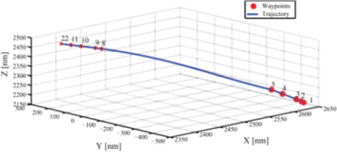
The time optimal trajectory of flight between Lisbon to Montreal (long-haul flight) contains 9 waypoints [initial waypoint (P1) → P14→ P3→ P4→ P5→ P10→ P11→ P13→ final waypoint (P26)], the distance between the initial and final waypoints in time optimal trajectory of this flight is 2772 nm. The comparison of travel time in different phases of flight for different trajectories and time optimal trajectory is shown in Table IX.
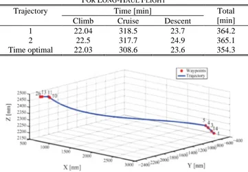
Table IX suggest that by using the time optimal trajectory in long-haul flight (Lisbon – Montreal) the aircraft reaches to the final waypoint from the initial waypoint 9.9 minutes faster than the first trajectory which saves 2.7% of the total travel time and 10.8 minutes faster than the second trajectory which save 2.9% of total travel time. The time optimal trajectory of long-haul flight in 3D is shown in Fig. 5.
TABLEIX
TOTAL TIME NEEDED IN DIFFERENT TRAJECTORIES
FOR LONG-HAUL FLIGHT
Trajectory Time [min] Total
[min] Climb Cruise Descent
1 22.04 318.5 23.7 364.2
2 22.5 317.7 24.9 365.1
Time optimal 22.03 308.6 23.6 354.3
Fig. 5. 3D time optimal trajectory in geocentric coordinates for long-haul flight
In Fig. 5 the blue curve is the time optimal trajectory and the red circles around it are the waypoints of the
trajectory. In this long-haul flight, the cruise phase is large compare to its climb and descent phases, thus in the fig. of time optimal trajectory for this flight the waypoints in the climb and descent phases are seems too close to each other.
V.
Conclusion
This paper is based on finding the time optimal trajectory of climb, cruise, and descent phases of the flight, but ignores the take-off and landing phases of the flight. In this study, several steps were made in order to achieve a complete trajectory from predefined 4D waypoint networks that optimize the total travel time.
This study uses Dijkstra’s single source shortest path algorithm in order to find the time optimal trajectory. Later on, this time optimal trajectory was used to compare with the existing 2 trajectories of different length (short, medium and long-haul) of flights.
The analysis results show promising potential for reduction of travel time in different flights via using the Dijkstra’s single source shortest path algorithm, across a range of common aircrafts and routes. The results suggest that by flying time optimal trajectory for short-haul flight, it is possible to save 2.7 − 3.7 minutes of travel time which is equivalent to 2.4 − 3.2 % of total travel time. In medium-haul flight by flying the time optimal trajectory the travel time was reduced by 4.2 − 5.5 minutes or 1.9 – 2.6% of total travel time. For long-haul flight, it is possible to save 9.9 − 10.8 minutes or 2.7 − 2.9% of total travel time by flying the time optimal trajectory. In general, the savings of the travel time are proportional to the trip lengths, and depends on the aircraft types. Despite of the fact that the algorithm has proven reliable to find the time optimal trajectory from pre-defined 4D waypoint networks, there is still room for improvement. By using more trajectories with different cruise altitude in the networks more travel time can be saved, as there will be more waypoints to choose from. However, this approach is not well suited for online trajectory optimization as the waypoint networks need to be pre-defined which requires some amount of time. But this can be solved by generating the waypoint networks by direct optimal control methods.
In addition, a realistic wind model and Air traffic control (ATC) restrictions can be imposed on the 4D waypoint networks to model more realistic flight.
Acknowledgements
This research work was conducted in the Aeronautics and Astronautics Research Group (AeroG) of the Associated Laboratory for Energy, Transports and Aeronautics (LAETA).
References
[1] Roberson B, "Fuel Conservation Strategies: Cost Index Explained," Boeing, 2007, pp. 26-28.
[2] Bryson A. E and Ho Y. C, "Applied Optimal Control: Optimization, Estimation and, Control", Taylor & Francis, New York, 1975.
[3] Betts, J.T., “Survey of numerical methods for trajectory optimization” Journal of Guidance, Control and Dynamics, 1998, pp. 193-207.
[4] Pontryagin, L.S., V.G. Boltyanskii, R.V. Gamkrelidze, E.F. Mishchenko. The Mathematical Theory of Optimal Processes, Wiley-Interscience, New-York, 1962.
[5] Von Stryk, O. and R. Bulirsch. “Direct and indirect methods for trajectory optimization”, Annals of Operations Research, 37, 1992, pp. 357-373.
[6] Hull, D.G., “Conversion of Optimal Control Problems into Parameter Optimization Problems”, Journal of Guidance, Control, and Dynamics, 1997, pp. 57-60.
[7] Schwartz, A. and E. Polak, “Consistent approximations for Optimal Control Problems Based on Runge-Kutta Integration”, SIAM Journal on Control and optimization, vol.34, No.4, 1996, pp. 1235-1269.
[8] Hargraves, C.R. and S.W. Paris, “Direct Trajectory Optimization Using Nonlinear Programming and Collocation”, Journal of Guidance, Control and Dynamics, vol. 10, No.4, 1987, pp. 338-342.
[9] Bousson, K. “Chebyshev pseudospectral trajectory optimization of differential inclusion models”, SAE World Aviation Congress, Montreal, Canada, paper no. 2003-01-3044, 2003.
[10] Fahroo, F. and I.M. Ross, “Direct trajectory optimization by a Chebyshev pseudospectral method”, Journal of Guidance, Control and Dynamics, 2002, pp. 160-166.
[11] Bousson K. and Machado P, "4D Flight Trajectory Generation and Tracking for Waypoint-Based Aerial Navigation," WSEAS transactions on system and control, Vol 8, No 3, july 2013, pp 105-119.
[12] Boukraa, D., Bestaoui, Y., Azouz, N., Three Dimensional Trajectory Generation for an Autonomous Plane, (2014) International Journal on Numerical and Analytical Methods in Engineering (IRENA), 2 (4), pp. 144-154.
[13] Bousson, K., Gameiro, T., A Quintic Spline Approach to 4D Trajectory Generation for Unmanned Aerial Vehicles, (2015) International Review of Aerospace Engineering (IREASE), 8 (1), pp. 1-9.
[14] Devika, K., Thomas, S., Path Planning for Conflict Resolution in Free Flight System: Optimization Based on Linear Programming, (2016) International Review of Aerospace Engineering (IREASE), 9 (1), pp. 1-6.
[15] Cormen T. H, Leiserson C. E, Rivest R. L and Stein C, "Introduction to algorithms", London, England: The MIT press, 2009, pp. 658-659.
[16] Hart C, "Graph Theory Topics in Computer Networking," (2013, pp 13-20).
[17] Dasgupta S, Papadimitriou C. H and Vazirani U. V, "Algorithms", McGraw-Hill, New York, July 18, 2006, pp. 112-118.
[18] Seemkooei A. A, "Comparison of different algorithm to transform geocentric to geodetic coordinates," Survey Review 36, October 2002, pp 627-632.
[19] EUROCONTROL "Aircraft Performance Summary Tables for the Base of Aircraft Data (BADA)," Eurocontrol Experimental Centre, Revision 3.4, June 2002.
[20] "SkyVector," Website Available: https://skyvector.com/. [Accessed October 2015].
Authors’ information
Avionics & Control Laboratory, Department of Aerospace sciences,
University of Beira Interior, 6201-001, Covilhã, Portugal. E-mails: kawser.ah91@gmail.com
bousson@ubi.pt
Kawser Ahmed received an Integrated Master's degrees in aeronautical engineering from University of Beira interior, Covilhã, Portugal in 2016. Currently is a PhD student in Department of Aerospace sciences at the University of Beira interior, Covilhã, Portugal, since September 2016. His current research includes optimal control, and trajectory optimization applied to fuel saving and environmental impact reduction. Eng. Ahmed is also a research member at the LAETA - Associated Laboratory for Energy, Transports, and Aeronautics.
K. Bousson received a MEng degree in aeronautical engineering from the Ecole Nationale de l’Aviation Civile (ENAC) in 1988, a MSc degree in computer science (with emphasis on artificial intelligence) from Paul Sabatier University in 1989, and a PhD degree in control & computer engineering from the Institut National des Sciences Appliquées (INSA) in 1993, all in Toulouse, France. He was a researcher at the LAAS Laboratory of the French National Council for Scientific Research (CNRS) in Toulouse, from 1993 to 1995, and has been a professor in the Department of Aerospace Sciences at the University of Beira Interior, Covilhã, Portugal, since 1995, and member of LAETA (Associated Laboratory for Energy, Transports, and Aeronautics). His current research activities include trajectory optimization & control of aerospace vehicles, nonlinear filtering and control of uncertain and chaotic systems, and machine learning. Dr. Bousson is a Member of the Portuguese Association for Automatic Control (APCA) and a Senior Member of the American Institute of Aeronautics and Astronautics (AIAA).