Deterministic Imputation in Multienvironment Trials

(1)

Volume 2013, Article ID 978780,17pages http://dx.doi.org/10.1155/2013/978780

Research Article

Deterministic Imputation in Multienvironment Trials

Sergio Arciniegas-Alarcón,

1

Marisol García-Peña,

1

Wojtek Janusz Krzanowski,

2

and Carlos Tadeu dos Santos Dias

1

1_{Departamento de Ciˆencias Exatas, Universidade de S˜ao Paulo/ESALQ, Cx.P.09, CEP. 13418-900, Piracicaba, SP, Brazil}

2_{College of Engineering, Mathematics and Physical Sciences Harrison Building, University of Exeter, North Park Road,}

Exeter, EX4 4QF, UK

Correspondence should be addressed to Sergio Arciniegas-Alarc´on; sergio.arciniegas@gmail.com

Received 26 June 2013; Accepted 16 August 2013

Academic Editors: A. Escobar-Gutierrez and W. P. Williams

Copyright © 2013 Sergio Arciniegas-Alarc´on et al. This is an open access article distributed under the Creative Commons Attribution License, which permits unrestricted use, distribution, and reproduction in any medium, provided the original work is properly cited.

This paper proposes five new imputation methods for unbalanced experiments with genotype by-environment interaction (𝐺 × 𝐸). The methods use cross-validation by eigenvector, based on an iterative scheme with the singular value decomposition (SVD) of a matrix. To test the methods, we performed a simulation study using three complete matrices of real data, obtained from𝐺 × 𝐸 interaction trials of peas, cotton, and beans, and introducing lack of balance by randomly deleting in turn 10%, 20%, and 40% of the values in each matrix. The quality of the imputations was evaluated with the additive main effects and multiplicative interaction model (AMMI), using the root mean squared predictive difference (RMSPD) between the genotypes and environmental parameters of the original data set and the set completed by imputation. The proposed methodology does not make any distributional or structural assumptions and does not have any restrictions regarding the pattern or mechanism of missing values.

1. Introduction

In plant breeding, multienvironment trials are important for testing the general and specific adaptations of cultivars. A cultivar developed in different environments will show significant fluctuations of performance in production relative to other cultivars. These changes are influenced by different environmental conditions and are referred to as genotype-by-environment interactions, or𝐺×𝐸. Often,𝐺×𝐸experiments are unbalanced because several genotypes are not tested in some environments. A common way of analyzing this type of study is by imputing the missing values and then apply-ing established procedures on the completed data matrix (observed + imputed), for example, the additive main effects and multiplicative interaction model—AMMI—or factorial regression [1–5]. An alternative approximation is to work with the incomplete data using a mixed model with estimates based on maximum likelihood [6].

Several imputation methods have been suggested in the literature to solve the problem of missing values. One of the first was made by Freeman [7], who suggested imputing the

(2)

that combines the singular value decomposition (SVD) of a matrix with the EM algorithm, obtaining results very useful for experiments in which the alternating least squares have some problems, for instance, convergence failures [18]. Recently, Bergamo et al. [19] proposed a distribution-free multiple imputation method that was assessed by Arciniegas-Alarcón [20] and compared by Arciniegas-Alarcón and Dias [21] with algorithms that use fixed effects models in a simulation study with real data. Meanwhile, a determinis-tic imputation method without structural or distributional assumptions for multienvironment experiments was pro-posed by Arciniegas-Alarcón et al. [22]. The method uses a mixture of regression and lower-rank approximation. Finally, other studies to analyze multienvironment experiments with missing values can be found in the literature. For example, methodologies for stability analysis have been studied by Raju and Bhatia [23] and Raju et al. [24,25]. Recently, Pereira et al. [26], Rodrigues et al. [27], and Rodrigues [28] assessed the robustness of joint regression analysis and AMMI models without the use of data imputation.

Given the historical information about data imputation in experiments, and specifically in two-factor𝐺 × 𝐸 exper-iments, the objective of the present paper is to propose a deterministic imputation algorithm without distributional or structural assumptions, using an extension of the cross-validation by eigenvector method presented by Bro et al. [29].

2. Materials and Methods

2.1. Data Imputation Using the Cross-Validation by Eigenvector Method. The cross-validation method was presented by Bro et al. [29] to find the optimum number of principal compo-nents in any data set that can be arranged in a matrix form. In this approximation, principal component analysis (PCA) models are calculated with one or several samples left out and the model is used to predict these samples. The method used cross-validation “leave-one-out” and the same study showed it to be more efficient than other well-known methodologies used in multivariate statistics, such as those presented by Wold [30] and Eastment and Krzanowski [31]. Because of this finding, Arciniegas-Alarc´on et al. [32] used the method to determine the best AMMI models in(𝐺 × 𝐸)experiments. This methodology is now presented.

Step 1. Consider the𝑛 × 𝑝matrixXwith elements𝑥_𝑖𝑗,(𝑖 =

1, . . . , 𝑛; 𝑗 = 1, . . . , 𝑝). The matrix is divided into disjoint groups, each group is deleted in turn (leave-one-out), and a PCA model(T,P)is obtained from the remainder by solving

min󵄩󵄩󵄩󵄩󵄩X(−𝑖)−TP𝑇󵄩󵄩󵄩󵄩󵄩2_𝑚 (1)

with𝑚 ≤min(𝑛 − 1, 𝑝 − 1). HereX(−𝑖)represents the matrix after deleting the𝑖th group (leave-one-out),‖ ⋅ ‖2defines the squared Frobenius norm,P𝑇P = I, andT,Pare scores and loadings matrices with dimensions(𝑛 − 1) × 𝑚and𝑝 × 𝑚 respectively, where 𝑝is the number of columns and 𝑚 is the number of components. Note that, in this method the deleted group corresponds to the𝑖th row ofXand according

to Smilde et al. [33] the model (1) can be rewritten in terms of the singular value decomposition (SVD)

X(−𝑖)=UDV𝑇=

𝑚

∑

𝑘=1

u_(𝑘)𝑑_𝑘k₍_k₎𝑇, (2)

whereU = [u₁,u₂, . . . ,u_𝑚],V = [k₁,k₂, . . . ,k_𝑚],D =

diag[𝑑₁, 𝑑₂, . . . , 𝑑_𝑚],T=UD,andP=V.

Step 2. Estimate the score

t(−𝑗)𝑇=x(−𝑗)𝑇_𝑖 P(−𝑗)(P(−𝑗)𝑇P(−𝑗))−1, (3)

whereP(−𝑗)𝑇is the loading matrix found inStep 1with the𝑗th row excluded.x_𝑖(−𝑗)𝑇is a row vector containing the𝑖th row of

Xexcept for the𝑗th element.

Step 3. Estimate the element𝑥_𝑖𝑗by

̂𝑥(𝑚)

𝑖𝑗 =t(−𝑗)𝑇p𝑇𝑗, (4)

p_𝑗is the𝑗th row ofP.

Step 4. Find the prediction error of the(𝑖𝑗)th element,𝑒(𝑚)_𝑖𝑗 =

𝑥𝑖𝑗− ̂𝑥(𝑚)𝑖𝑗 .

Step 5. Obtain the criterion value

PRESS(𝑚) =

𝑛

∑

𝑖=1 𝑝

∑

𝑗=1(𝑒

(𝑚)

𝑖𝑗 )2. (5)

In order to make the imputation of missing values in the matrix from(𝐺×𝐸)experiments, a change is proposed in the method following the work of Krzanowski [34], Bergamo et al. [19], and Arciniegas-Alarc´on et al. [22] using the singular value decomposition of a matrix [35].

Initially, suppose that 𝑛 ≥ 𝑝 and the matrix X has several missing values; in the case𝑛 < 𝑝, the matrix should first be transposed. The missing values are replaced by their respective column means𝑥_𝑗, and after this has been done the matrix is standardized by columns, subtracting 𝑥_𝑗 and dividing by𝑠_𝑗(where𝑥_𝑗and𝑠_𝑗represent, resp., the mean and the standard deviation of thejth column). The eigenvector procedure using the SVD in expressions (2)–(4) is applied to the standardized matrix to find the imputation of the(𝑖, 𝑗) element, denoted by ̂𝑥(𝑚)_𝑖𝑗 . After the imputation, the matrix must be returned to its original scale,𝑥_𝑖𝑗= 𝑥_𝑗+ 𝑠_𝑗̂𝑥(𝑚)_𝑖𝑗 .

(3)

the process to run until convergence has been achieved. As regards to the computing effort, convergence can depend strongly on the size of matrix analyzed and also on the data structure (size of correlations, proportion of missing values, etc.), but in, for instance, the SVD method of Hastie et al. [36], convergence is achieved usually between 5 and 6 iterations, and in the Bergamo et al. [19] method it is achieved in between 20 and 50 iterations maximum.

On the other hand, the data imputation depends directly on (2) and (3). Equation (2) needs prior choice of the number of components(𝑚) to extract from the SVD. Krzanowski [34] and Bergamo et al. [19] took𝑚 = min{𝑛 − 1, 𝑝 − 1} with the objective of using the maximum amount of available information, but Hedderley and Wakeling [37] affirmed that if the estimation is based on the choice of a unique fixed number of dimensions, some of the lower dimensions may be essentially random. This can influence the imputation within an iterative scheme and can lead to the estimates becoming trapped in a cycle, hence preventing convergence. To solve this problem, they suggested including a test to check on the convergence rate, and in case a specific criterion is not being attained the number of dimensions should be reduced. Another option that has satisfactory results, suggested by Josse et al. [38] to choose an optimum𝑚, is through cross-validation based uniquely on the observed data. However, the computational cost of this option is likely to be high.

Taking into account all the above mentioned in the present study, for imputation of each missing value of the matrixX the value of𝑚in (2) is allowed to be different in each SVD calculated and is chosen according to the criterion used by Arciniegas-Alarc´on et al. [22]. Thus,𝑚is chosen such

that((∑𝑚_𝑘=1𝑑2_𝑘)/(∑_𝑘=1min{𝑛−1,𝑝−1}𝑑2_𝑘)) ≈ 0.75. Moreover, in (3),

the Moore-Penrose generalized inverse can be used instead of the classic inverse matrix as was studied in cross-validation by Dias and Krzanowski [39].

In this research, five imputation methods have been assessed. They are denoted Eigenvector0, Eigenvector1, Eigenvector2, Eigenvector3, and Eigenvector where the num-ber indicates the numnum-ber of iterations used while in the case of Eigenvector the process is iterated until convergence is achieved in the imputations.

These imputation methods are all deterministic impu-tations, and they have the advantage over other stochastic imputation methods (parametric multiple imputations) that the imputed values are uniquely determined and will always yield the same results when applied to a given data set. This is not necessarily true for the stochastic imputation methods [40].

2.2. The Data. To assess the imputation methods we used three data sets, published in Cali´nski et al. [41, page 227], Farias [42, page 115], and Flores et al. [43, page 274], respec-tively. In each case the data were obtained from a randomized complete block design with replication, and each reference offers an excellent description of the design if further details are required.

The first data set “Cali´nski” comprises an 18×9 matrix, for 18 pea varieties assessed in 9 different locations in Poland.

The experiment was conducted by the Research Center for Cultivar Testing, Slupia Wielka, and the studied variable was mean yield (dt/ha).

The second data set “Farias” was obtained from Upland cotton variety trials (Ensaio Estadual de Algodoeiro Herbáceo) in the agricultural year 2000/01, part of the cotton improvement program for the Cerrado conditions. The experiments assessed 15 cotton cultivars in 27 locations in the Brazilian states of Mato Grosso, Mato Grosso do Sul, Goiás, Minas Gerais, Rondônia, Maranhão, and Piau´ı. The studied variable was yield seed cotton (kg/ha).

The third data set “Flores” is in a 15 × 12 matrix, for 15 bean varieties assessed in 12 environments in Spain. The experiments were conducted by RAEA—Red Andaluza de Experimentaci´on Agraria—where the studied variable was mean yield (kg/ha).

The three data matrices contained just the mean yield for each genotype in each environment, but the proposed methods work for any data set arranged in matrix form. For example, if information about the replications is available, an approach suggested by Bello [44] is to write the experiment in terms of a classic linear regression model in order to obtain the response vector and the design matrix, and then to join them into a single matrix and apply the proposed methods in this paper.

2.3. Simulation Study. Each original data matrix (“Cali´nski”, “Farias”, and “Flores”) was submitted to random deletion of values at the three rates 10%, 20%, and 40%. The process was repeated in each data set 1000 times for each percentage of missing values, giving a total of 3000 different matrices with missing values. Altogether, therefore, 9000 incomplete data sets were available, and for each one the missing values were imputed with the 5 Eigenvector algorithms described above using computational code in R [45].

The random deletion process for a matrixX(𝑛 × 𝑝)was conducted as follows. Random numbers between 0 and 1 were generated in R with therunif_{function. For a fixed}𝑟_value

(0 < 𝑟 < 1), if the(𝑝𝑖 + 𝑗)th random number was lower than𝑟, then the element in the(𝑖+1, 𝑗)position of the matrix was deleted (𝑖 = 0, 1, . . . , 𝑛; 𝑗 = 1, . . . , 𝑝). The expected proportion of missing values in the matrix will be𝑟[34]. This technique was used with𝑟 = 0.1,0.2and0.4(i.e., 10%, 20%, and 40%).

2.4. Comparison Criteria. In general, the objective after imputation is to estimate model parameters from the com-plete table of information. One of the models frequently used in genotype-by-environmental trials is the AMMI model [46, 47], and for this reason the algorithms proposed in this paper will be compared through the genotypic and environmental parameters of the fitted AMMI models using the root mean squared predictive difference—RMSPD [39]. The AMMI model is first briefly presented.

The usual two-way ANOVA model to analyze data from genotype-by-environment trials is defined by

(4)

(𝑖 = 1, . . . , 𝑛; 𝑗 = 1, . . . , 𝑝) where 𝜇, 𝑎_𝑖, 𝑏_𝑗, (𝑎𝑏)_𝑖𝑗, and

𝑒𝑖𝑗 are respectively, the overall mean, the genotypic and

environmental main effects, the genotype-by-environment interaction, and an error term associated with the𝑖th geno-type and jth location. It is assumed that all effects except the error are fixed effects. The following reparametrization constraints are imposed: ∑_𝑖(𝑎𝑏)_𝑖𝑗 = ∑_𝑗(𝑎𝑏)_𝑖𝑗 = ∑_𝑖𝑎_𝑖 =

∑𝑗𝑏𝑗 = 0. The AMMI model implies that interactions can

be expressed by the sum of multiplicative terms. The model is given by

𝑦𝑖𝑗= 𝜇 + 𝑎𝑖+ 𝑏𝑗+ 𝜃1𝛼𝑖1𝛽𝑗1+ 𝜃2𝛼𝑖2𝛽𝑗2+ ⋅ ⋅ ⋅ + 𝑒𝑖𝑗, (7) where 𝜃_𝑙, 𝛼_𝑖𝑙, and𝛽_𝑗𝑙(𝑙 = 1, 2, . . . ,min(𝑛 − 1, 𝑝 − 1)) are estimated by the SVD of the matrix of residuals after fitting the additive part. 𝜃_𝑙 is estimated by the𝑙th singular value of the SVD,𝛼_𝑖𝑙 and𝛽_𝑗𝑙 are estimated by the genotypic and environmental eigenvector values corresponding to𝜃_𝑙.

Alternating regressions can be used in place of the SVD [48]; depending on the number of multiplicative terms, these models may be called AMMI0, AMMI1, and so forth.

An inherent requirement of the AMMI model is prior specification of the number of multiplicative components [49–51]. Rodrigues [28] made an exhaustive analysis of the related literature and concluded that usually two or three components can be used because, in general, one component is not enough to capture the entire pattern of response in the data, but with more than three components there are obvious visualization problems, and a huge quantity of noise is liable to be captured.

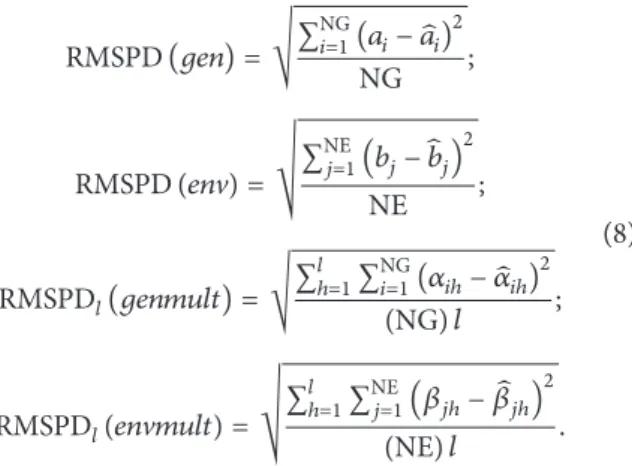
So, for the original matrices “Cali´nski”, “Farias”, and “Flores”, we fitted the AMMI2 and AMMI3 models. The same models were then fitted for each one of the 9000 sets of data that had been completed by imputation, and each set of parameters was compared with its corresponding set from the original data by using the RMSPD in the following way:

RMSPD(𝑔𝑒𝑛) = √∑ NG

𝑖=1(𝑎𝑖− ̂𝑎𝑖)2

NG ;

RMSPD(𝑒𝑛V) = √

∑NE

𝑗=1(𝑏𝑗− ̂𝑏𝑗)2

NE ;

RMSPD_𝑙(𝑔𝑒𝑛𝑚𝑢𝑙𝑡) = √∑

𝑙

ℎ=1∑NG𝑖=1(𝛼𝑖ℎ− ̂𝛼𝑖ℎ)2

(NG) 𝑙 ;

RMSPD_𝑙(𝑒𝑛V𝑚𝑢𝑙𝑡) = √

∑𝑙

ℎ=1∑NE𝑗=1(𝛽𝑗ℎ− ̂𝛽𝑗ℎ)2

(NE) 𝑙 . (8)

Here RMSPD(𝑔𝑒𝑛)represents the RMSPD among the esti-mated parameters for genotype main effects from the original data 𝑎_𝑖 and the corresponding parameters obtained from the completed data sets by imputation ̂𝑎_𝑖. RMSPD(𝑒𝑛V)

represents the RMSPD among the estimated parameters for environments main effects from the original data 𝑏_𝑗 and the corresponding parameters obtained from the com-pleted data sets by imputation̂𝑏_𝑗. RMSPD_𝑙(𝑔𝑒𝑛𝑚𝑢𝑙𝑡) rep-resents the equivalent RMSPD for the pairs of estimated

parameters of genotype multiplicative components𝛼_𝑖ℎ, ̂𝛼_𝑖ℎ. RMSPD_𝑙(𝑒𝑛V𝑚𝑢𝑙𝑡)represents the equivalent RMSPD for the

pairs of estimated parameters of environments multiplicative components 𝛽_𝑗ℎ, ̂𝛽_𝑗ℎ. In the statistics, NG represents the number of genotypes, NE the number of environments, and

𝑙 = 2or 3 depending on the considered model AMMI2 or AMMI3.

The best imputation method is the one with the lowest values of RMSPD in each case. Summarizing, in each simu-lated data set with missing values, we applied the methods Eigenvector, Eigenvector0, Eigenvector1, Eigenvector2, and Eigenvector3 and, then, in the completed data (observed + imputed) we fitted AMMI2, AMMI3 models for the calculation of the respectively RMSPD statistics. In order to visualize any differences more readily, the RMSPD values were standardized and the comparison was made directly. Note that because of the standardized scale, the values of the statistics can be either positive or negative.

3. Results

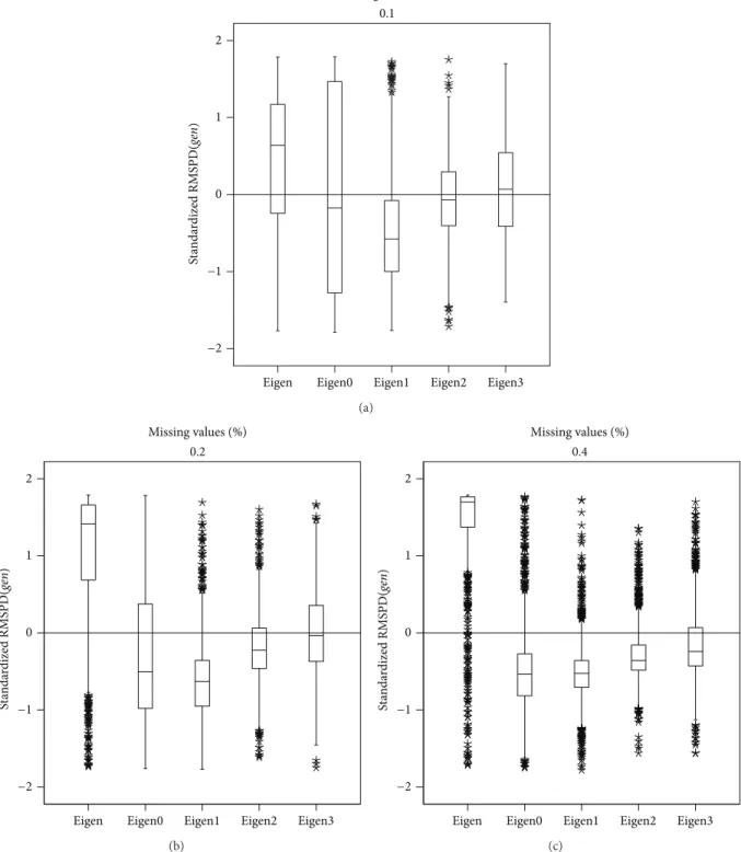
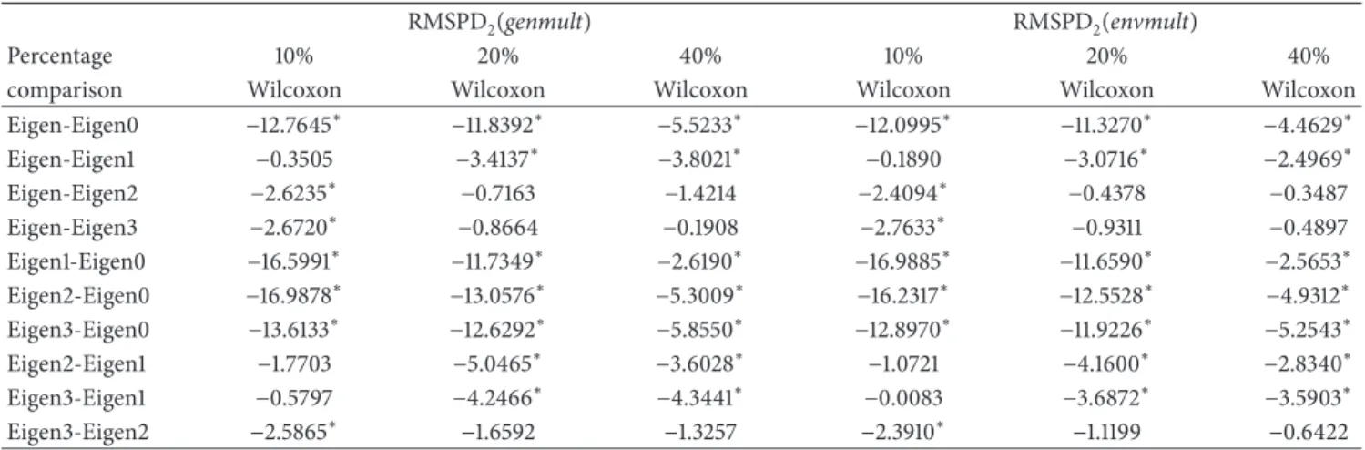
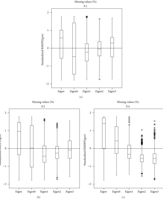
3.1. Polish Pea Data. Figure 1shows the RMSPD(𝑔𝑒𝑛)

dis-tribution on the standardized scale for the “Cali´nski” data set, showing each imputation method and each percentage. It can be seen that the Eigenvector distribution is left asym-metric and this asymmetry increases as the missing values percentage increases. In general, the Eigenvector distribution has values above zero and when the number of missing values increases, it is concentrated above one. This means that this method had the biggest differences among the additive genotypic parameters of the real and completed (by imputation) data.

The best method according to RMSPD(𝑔𝑒𝑛)is Eigenvec-tor1, the method with just one iteration. This method has the smallest median for the 10% and 20% percentages. In the 40% percentage the medians of Eigenvector0 and Eigenvector1 are practically the same in the figure, but Eigenvector1 continues be preferable because it has the smallest dispersion. So, Eigenvector1 gave the smallest differences between the additive genotypic parameters of the real and completed data.

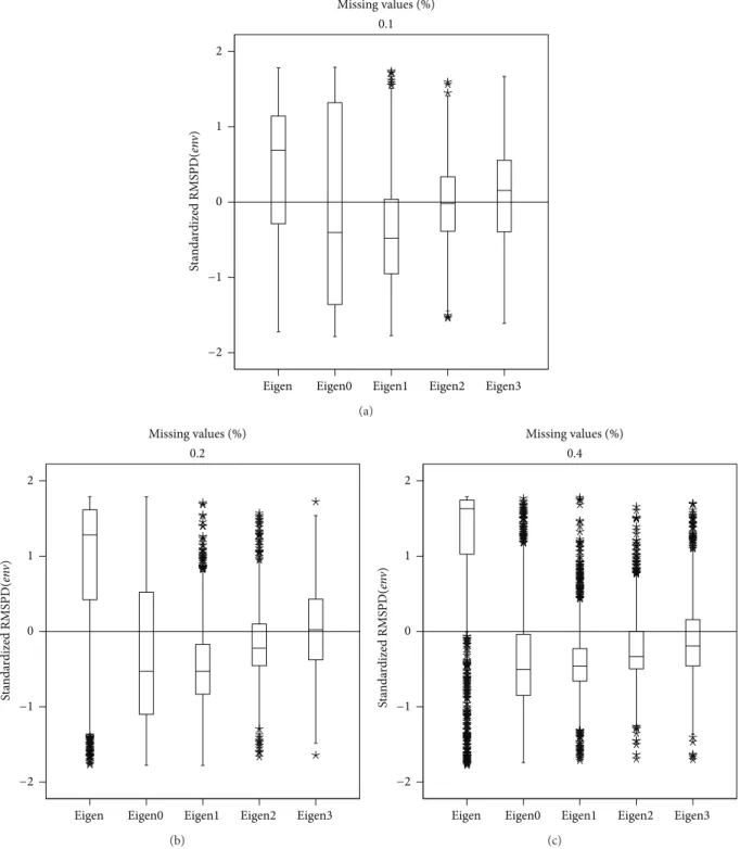
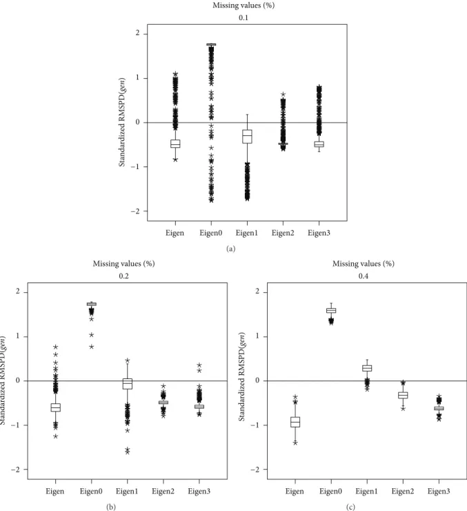
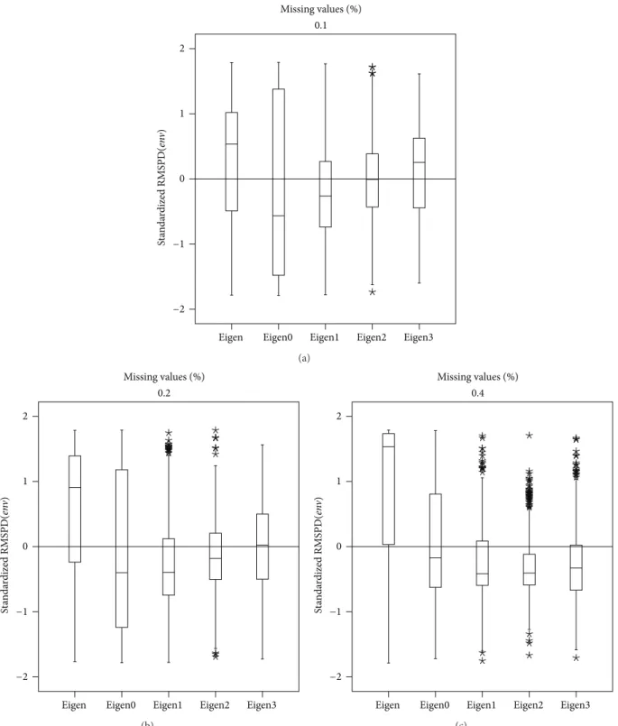
Figure 2 shows the RMSPD(𝑒𝑛V) on the standardized

scale for the “Cali´nski” data set. It shows very similar behaviour to that of RMSPD(𝑔𝑒𝑛). Again the Eigenvector method presents the biggest differences among the additive environment parameters of the real and completed data because of the algorithm that maximizes the RMSPD(𝑒𝑛V).

In this case, the RMSPD(𝑒𝑛V)is minimized with Eigenvector0

and Eigenvector1, and in all the percentages of missing values the two have nearly equal medians. However, Eigenvector1 has the smallest dispersion and that makes this again the method of choice.

The box plot analysis was useful in determining

the best imputation method for the RMSPD(𝑔𝑒𝑛)

and RMSPD(𝑒𝑛V) distributions, but in the case of

RMSPD₂(𝑒𝑛V𝑚𝑢𝑙𝑡), RMSPD₂(𝑔𝑒𝑛𝑚𝑢𝑙𝑡), RMSPD₃(𝑔𝑒𝑛𝑚𝑢𝑙𝑡)

and RMSPD₃(𝑒𝑛V𝑚𝑢𝑙𝑡), a more formal analysis can be used

(5)

Missing values (%)

2

1

0

−1

−2

0.1

Eigen Eigen0 Eigen1 Eigen2 Eigen3

St

an

da

rdized RMS

PD(

gen

)

(a)

Missing values (%)

2

1

0

−1

−2

0.2

St

an

da

rdized RMS

PD(

gen

)

(b)

Missing values (%) 0.4

2

1

0

−1

−2

St

an

da

rdized RMS

PD(

gen

)

(c)

Figure 1: Box plot of the RMSPD(𝑔𝑒𝑛)distribution in Cali´nski data set.

Table 1shows the Friedman test statistics. It can be seen that a significant difference exists among the imputation methods for the 10% and 20% percentage of missing values, but with 40% the five methods have equivalent results. After the general test, it is necessary to make multiple pairwise comparisons for the two lower percentages.

Table 2shows the Wilcoxon test to find the methods that are different. When RMSPD₂(𝑔𝑒𝑛𝑚𝑢𝑙𝑡) for 10% was used,

(6)

Missing values (%)

2

1

0

−1

−2

0.1

St

an

da

rdized RMS

PD(

en

v

)

(a)

Missing values (%)

2

1

0

−1

−2

0.2

St

an

da

rdized RMS

PD(

en

v

)

(b)

Missing values (%)

2

1

0

−1

−2

0.4

St

an

da

rdized RMS

PD(

en

v

)

(c)

Figure 2: Box plot of the RMSPD(𝑒𝑛V)distribution in Cali´nski data set.

Table 1: Friedman test for the standardized RMSPD_𝑙(⋅)—Cali´nski data set.

Perc.

Statistic

RMSPD2(genmult) RMSPD2(envmult) RMSPD3(genmult) RMSPD3(envmult)

Friedman 𝑃value Friedman 𝑃value Friedman 𝑃value Friedman 𝑃value

10% 15.6256 0.0036 34.4896 0.0000 34.9368 0.0000 30.4928 0.0000

20% 10.7848 0.0291 11.3688 0.0227 16.7144 0.0022 11.1104 0.0254

(7)

Table 2: Wilcoxon test for the standardized RMSPD₂(⋅)—Cali´nski data set.

RMSPD₂(genmult) RMSPD₂(envmult)

Percentage 10% 20% 10% 20%

comparison Wilcoxon Wilcoxon Wilcoxon Wilcoxon

Eigen-Eigen0 −0.2913 −2.4166∗ −0.8459 −1.7890

Eigen-Eigen1 −3.4322∗ −2.6145∗ −4.5972∗ −1.5540

Eigen-Eigen2 −1.0087 −1.0783 −2.0225∗ −0.1250

Eigen-Eigen3 −1.3178 −2.0335∗ −2.4155∗ −0.7970

Eigen1-Eigen0 −2.0468∗ −0.1261 −2.8270∗ −0.5490

Eigen2-Eigen0 −0.2997 −1.6703 −0.2598 −2.0420∗

Eigen3-Eigen0 −0.3213 −1.3256 −0.0852 −1.6410

Eigen2-Eigen1 −3.3075∗ −2.7537∗ −4.3006∗ −2.5030∗

Eigen3-Eigen1 −3.5483∗ −2.2389∗ −5.0405∗ −2.3590∗

Eigen3-Eigen2 −0.4955 −0.0203 −0.9271 −0.6170

∗_{Significant difference 5%.}

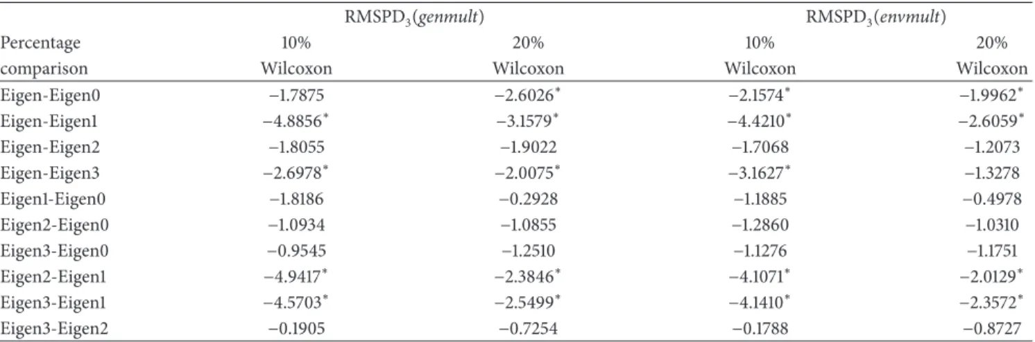
Table 3: Wilcoxon test for the standardized RMSPD₃(⋅)—Cali´nski data set.

RMSPD₃(genmult) RMSPD₃(envmult)

Percentage 10% 20% 10% 20%

comparison Wilcoxon Wilcoxon Wilcoxon Wilcoxon

Eigen-Eigen0 −1.7875 −2.6026∗ −2.1574∗ −1.9962∗

Eigen-Eigen1 −4.8856∗ −3.1579∗ −4.4210∗ −2.6059∗

Eigen-Eigen2 −1.8055 −1.9022 −1.7068 −1.2073

Eigen-Eigen3 −2.6978∗ −2.0075∗ −3.1627∗ −1.3278

Eigen1-Eigen0 −1.8186 −0.2928 −1.1885 −0.4978

Eigen2-Eigen0 −1.0934 −1.0855 −1.2860 −1.0310

Eigen3-Eigen0 −0.9545 −1.2510 −1.1276 −1.1751

Eigen2-Eigen1 −4.9417∗ −2.3846∗ −4.1071∗ −2.0129∗

Eigen3-Eigen1 −4.5703∗ −2.5499∗ −4.1410∗ −2.3572∗

Eigen3-Eigen2 −0.1905 −0.7254 −0.1788 −0.8727

because it minimizes the median and presents the smallest dispersion compared with Eigenvector and Eigenvector0. The five methods all present similar results for the 40% deletion rate.

Table 2shows the Wilcoxon test results for the 10% and 20% percentage of missing values using RMSPD₂(𝑒𝑛V𝑚𝑢𝑙𝑡).

There are significant differences among Eigenvector and Eigenvector2, Eigenvector3, and Eigenvector1 for the 10% deletion rate. Differences were found between Eigenvector1 and Eigenvector0, Eigenvector2 and Eigenvector3, respec-tively. For 20%, Eigenvector1 was different from Eigenvector2 and Eigenvector3; besides, there is a difference between Eigenvector0 and Eigenvector2.

However, Table 3 shows the Wilcoxon test results of the standardized RMSPD₃(𝑒𝑛V𝑚𝑢𝑙𝑡)and RMSPD₃(𝑔𝑒𝑛𝑚𝑢𝑙𝑡)

values. In the 10% and 20% imputation percentages, there were significant differences between Eigenvector1 and Eigen-vector, Eigenvector2 and Eigenvector3, respectively. Also, significant differences were detected between Eigenvector and the Eigenvector0 and Eigenvector3.

Finally, box plots were made for RMSPD₂(𝑒𝑛V𝑚𝑢𝑙𝑡),

RMSPD₃(𝑔𝑒𝑛𝑚𝑢𝑙𝑡), and RMSPD₃(𝑒𝑛V𝑚𝑢𝑙𝑡), but are not

pre-sented here because they have similar behaviour to those in

Figure 3, confirming that Eigenvector1 minimizes the median if it is compared with Eigenvector2 and Eigenvector3 and also has smaller dispersion than Eigenvector0. The method that always maximized all the statistics was Eigenvector, and for this reason it is the least recommended.

3.2. Brazilian Cotton Data. Figure 4shows the RMSPD(𝑔𝑒𝑛)

(8)

Missing values (%)

2

1

0

−1

−2

0.1

St

an

da

rdized RMS

P

D2

(

ge

nmu

lt

)

(a)

Missing values (%)

2

1

0

−1

−2

0.2

St

an

da

rdized RMS

P

D2

(

ge

nmu

lt

)

(b)

Figure 3: Box plot of the RMSPD₂(𝑔𝑒𝑛𝑚𝑢𝑙𝑡)distribution in Cali´nski data set.

Table 4: Friedman test for the standardized RMSPD_𝑙(⋅)—Farias data set.

Perc.

Statistic

10% 452.1168 0.0000 444.0952 0.0000 228.6352 0.0000 201.9368 0.0000

20% 313.0696 0.0000 295.0152 0.0000 193.6624 0.0000 173.3472 0.0000

40% 49.8712 0.0000 32.3296 0.0000 25.5240 0.0000 10.8736 0.0280

with Eigenvector2. Overall, when the missing values per-centage increases Eigenvector achieves the best performance, because it minimizes RMSPD(𝑔𝑒𝑛). A similar behaviour is shown for RMSPD(𝑒𝑛V), as can be observed inFigure 5.

Table 4 shows the Friedman test statistics for RMSPD₂(𝑔𝑒𝑛𝑚𝑢𝑙𝑡), RMSPD₂(𝑒𝑛V𝑚𝑢𝑙𝑡), RMSPD₃(genmult),

and RMSPD₃(𝑒𝑛V𝑚𝑢𝑙𝑡). There is a significant difference

among the imputation methods for all the percentages of missing values, so multiple pairwise comparisons were made with the Wilcoxon test.

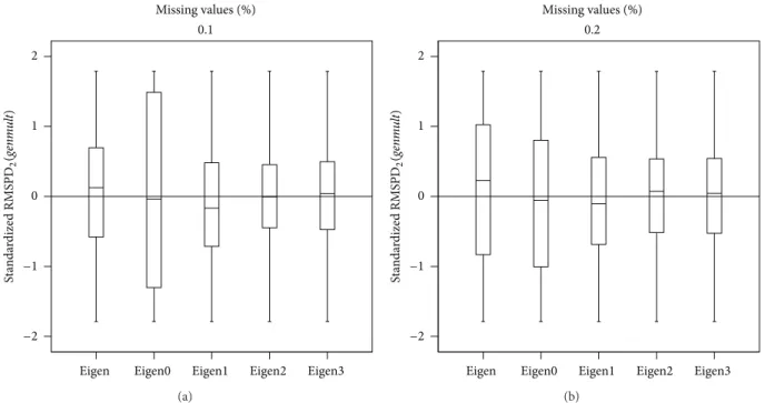
Table 5shows the Wilcoxon tests for RMSPD₂(𝑔𝑒𝑛𝑚𝑢𝑙𝑡) and RMSPD₂(𝑒𝑛V𝑚𝑢𝑙𝑡). They indicate that with 10%

impu-tation, the majority of the compared pairs have a significant difference, but, for example, Eigenvector1 is not significantly different from Eigenvector, Eigenvector2 or Eigenvector3. For the other two percentages, 20% and 40%, Eigenvector is not statistically different from Eigenvector2, and Eigenvector3 which have similar performances.

Table 6shows the Wilcoxon test for RMSPD₃(𝑒𝑛V𝑚𝑢𝑙𝑡).

With 10% imputation, Eigenvector0 is different from all the others, while for RMSPD₃(𝑔𝑒𝑛𝑚𝑢𝑙𝑡)at the same percentage, Eigenvector1 was statistically different from Eigenvector2. With 20% and 40% of imputation, Eigenvector is not different

from Eigenvector2 or Eigenvector3, and likewise Eigenvec-tor3 is not different from Eigenvector2.

In order to make a definitive conclusion, box plots were made for RMSPD₃(𝑔𝑒𝑛𝑚𝑢𝑙𝑡), RMSPD₃(𝑒𝑛V𝑚𝑢𝑙𝑡),

RMSPD₂(𝑔𝑒𝑛𝑚𝑢𝑙𝑡), and RMSPD₂(𝑒𝑛V𝑚𝑢𝑙𝑡), but just one

of them is presented because the distribution behaviour is similar for the others. FromFigure 6, it can be concluded that the methods that minimize the median in all the percentages are Eigenvector, Eigenvector2, and Eigenvector3, and Tables

5and6show that these methods are equivalent.

In summary, for the “Farias” data set, with the six stan-dardized statistics, Eigenvector always showed good results and is therefore the recommended one.

3.3. Spanish Beans Data. Figure 7shows the RMSPD(𝑔𝑒𝑛)

(9)

Table 5: Wilcoxon test for the standardized RMSPD₂(⋅)—Farias data set.

RMSPD₂(genmult) RMSPD₂(envmult)

Percentage 10% 20% 40% 10% 20% 40%

comparison Wilcoxon Wilcoxon Wilcoxon Wilcoxon Wilcoxon Wilcoxon

Eigen-Eigen0 −12.7645∗ −11.8392∗ −5.5233∗ −12.0995∗ −11.3270∗ −4.4629∗

Eigen-Eigen1 −0.3505 −3.4137∗ −3.8021∗ −0.1890 −3.0716∗ −2.4969∗

Eigen-Eigen2 −2.6235∗ −0.7163 −1.4214 −2.4094∗ −0.4378 −0.3487

Eigen-Eigen3 −2.6720∗ −0.8664 −0.1908 −2.7633∗ −0.9311 −0.4897

Eigen1-Eigen0 −16.5991∗ −11.7349∗ −2.6190∗ −16.9885∗ −11.6590∗ −2.5653∗

Eigen2-Eigen0 −16.9878∗ −13.0576∗ −5.3009∗ −16.2317∗ −12.5528∗ −4.9312∗

Eigen3-Eigen0 −13.6133∗ −12.6292∗ −5.8550∗ −12.8970∗ −11.9226∗ −5.2543∗

Eigen2-Eigen1 −1.7703 −5.0465∗ −3.6028∗ −1.0721 −4.1600∗ −2.8340∗

Eigen3-Eigen1 −0.5797 −4.2466∗ −4.3441∗ −0.0083 −3.6872∗ −3.5903∗

Eigen3-Eigen2 −2.5865∗ −1.6592 −1.3257 −2.3910∗ −1.1199 −0.6422

Table 6: Wilcoxon test for the standardized RMSPD₃(⋅)—Farias data set.

RMSPD3(genmult) RMSPD3(envmult)

Percentage 10% 20% 40% 10% 20% 40%

comparison Wilcoxon Wilcoxon Wilcoxon Wilcoxon Wilcoxon Wilcoxon

Eigen-Eigen0 −9.2191∗ −9.2224∗ −4.1232∗ −8.2742∗ −8.9679∗ −2.1050∗

Eigen-Eigen1 −1.1084 −2.2832∗ −3.3175∗ −0.1224 −2.2990∗ −2.0120∗

Eigen-Eigen2 −0.6928 −0.1061 −0.8429 −1.1718 −0.2890 −0.3286

Eigen-Eigen3 −0.9784 −0.1836 −0.2097 −1.7433 −0.2468 −0.5434

Eigen1-Eigen0 −11.1032∗ −8.6574∗ −1.0162 −10.6797∗ −8.5424∗ −0.2532

Eigen2-Eigen0 −11.7189∗ −9.8996∗ −3.5702∗ −11.2791∗ −9.5638∗ −2.5008∗

Eigen3-Eigen0 −9.8820∗ −9.3163∗ −4.3048∗ −8.8932∗ −9.1492∗ −2.7670∗

Eigen2-Eigen1 −2.2248∗ −3.7149∗ −3.0406∗ −1.4067 −3.5119∗ −2.6124∗

Eigen3-Eigen1 −1.5319 −2.3342∗ −3.5506∗ −0.5309 −2.4132∗ −2.8674∗

Eigen3-Eigen2 −0.3787 −0.2394 −0.9666 −0.8871 −0.2512 −0.0848

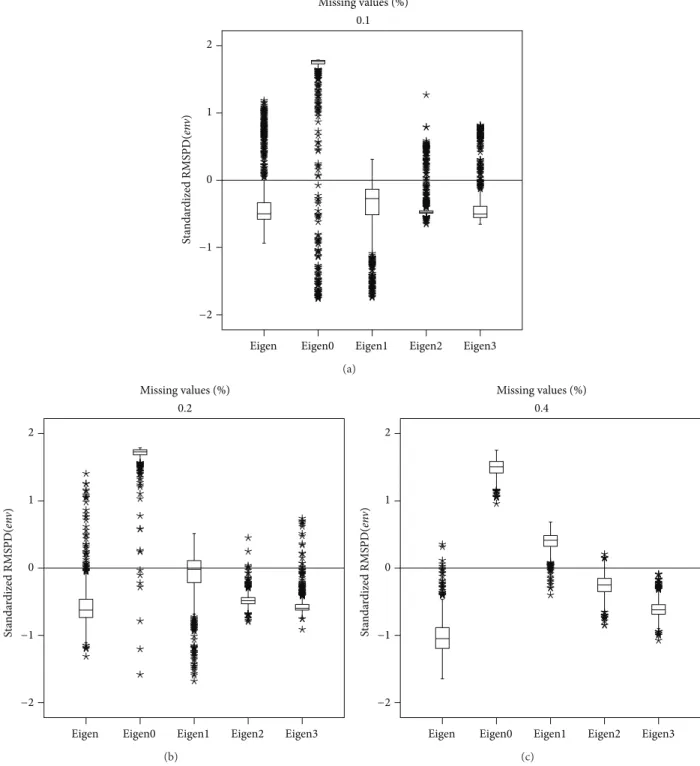
with 40% it is Eigenvector2, minimizing the median and taking the RMSPD(𝑔𝑒𝑛)distribution to the bottom of the standardized scale. Figure 8 presents a similar result, but using RMSPD(𝑒𝑛V). From the figure it can be said that

with 20% imputation, Eigenvector0 and Eigenvector1 have similar medians, but Eigenvector1 is preferred because it has the smallest dispersion. With RMSPD(𝑒𝑛V), Eigenvector0

has right asymmetric distributions and Eigenvector1, Eigen-vector2, and Eigenvector3 have approximately symmetric distributions.

Table 7 shows the Friedman test for the statistics RMSPD₂(𝑔𝑒𝑛𝑚𝑢𝑙𝑡), RMSPD₂(𝑒𝑛V𝑚𝑢𝑙𝑡), RMSPD₃(genmult),

and RMSPD₃(𝑒𝑛V𝑚𝑢𝑙𝑡). It can be seen that significant

differences exist among the methods only for 10% imputation. For this reason we restrict attention to this percentage.

Table 8 shows the 10 pairwise possible comparisons of imputation methods considering just 10% imputation and the statistics RMSPD₂(𝑔𝑒𝑛𝑚𝑢𝑙𝑡), RMSPD₂(𝑒𝑛V𝑚𝑢𝑙𝑡),

RMSPD₃(𝑔𝑒𝑛𝑚𝑢𝑙𝑡), and RMSPD₃(𝑒𝑛V𝑚𝑢𝑙𝑡). Taken

across the statistics all the methods are different except Eigenvector1 and Eigenvector0, but additionally, for

RMSPD₂(𝑔𝑒𝑛𝑚𝑢𝑙𝑡)the pair Eigenvector1 and Eigenvector2 and for RMSPD₃(𝑔𝑒𝑛𝑚𝑢𝑙𝑡) the pair Eigenvector2 and Eigenvector0 are not significantly different.

Finally, to make a definitive conclusion about the four analyzed statistics in Tables 7 and 8, the box plot for RMSPD₂(𝑔𝑒𝑛𝑚𝑢𝑙𝑡)is presented inFigure 9. Plots were made of the other three statistics, but are not presented here because the behaviour is similar. According to the box plot, the best method is Eigenvector0 because it minimizes the median.

4. Discussion

We have presented five imputation methods and tested them through a simulation study based on three multienvironment trials and using six statistics derived from RMSPD. Overall, for big trials (i.e., 450 observations in the data matrix) Eigenvector should be used under convergence, while for small trials (i.e., 162 or 180 observations in the data matrix) two cycles of the process are enough in order to obtain good results without convergence.

(10)

Missing values (%)

2

1

0

−1

−2

0.1

St

an

da

rdized RMS

PD(

gen

)

(a)

Missing values (%)

2

1

0

−1

−2

0.2

St

an

da

rdized RMS

PD(

gen

)

(b)

Missing values (%)

2

1

0

−1

−2

0.4

St

an

da

rdized RMS

PD(

gen

)

(c)

Figure 4: Box plot of the RMSPD(𝑔𝑒𝑛)distribution in Farias data set.

Table 7: Friedman test for the standardized RMSPD_𝑙(⋅)—Flores data set.

Perc.

Statistic

RMSPD₂(genmult) RMSPD₂(envmult) RMSPD₃(genmult) RMSPD₃(envmult)

10% 23.1512 0.0001 39.0136 0.0000 24.0736 0.0001 26.1888 0.0000

20% 5.0296 0.2843 2.2608 0.6879 1.8144 0.7698 1.0936 0.8953

(11)

Missing values (%)

2

1

0

−1

−2

0.1

St

an

da

rdized RMS

PD(

en

v

)

(a)

Missing values (%)

2

1

0

−1

−2

0.2

St

an

da

rdized RMS

PD(

en

v

)

(b)

Missing values (%)

2

1

0

−1

−2

0.4

St

an

da

rdized RMS

PD(

en

v

)

(c)

Figure 5: Box plot of the RMSPD(𝑒𝑛V)distribution in Farias data set.

were as expected, but one important outcome is that the iter-ative aspect of the proposed algorithms should be obligatory when missing values are imputed in𝐺 × 𝐸experiments.

So there is a natural question for the applied researcher: how to choose the appropriate Eigenvector imputation method for experiments with different size to those illustrated in this paper? The answer depends on the imputation objec-tive, because the imputation can be used in several ways: to establish one or more genotype-environment combinations

(12)

Missing values (%)

2

1

0

−1

−2

0.1

St

an

da

rdized RMS

P

D2

(

ge

nmu

lt

)

(a)

Missing values (%)

2

1

0

−1

−2

0.2

St

an

da

rdized RMS

PD

2

(

ge

nmu

lt

)

(b)

Missing values (%)

2

1

0

−1

−2

0.4

St

an

da

rdized RMS

PD

2

(

ge

nmu

lt

)

(c)

Figure 6: Box plot of the RMSPD₂(𝑔𝑒𝑛𝑚𝑢𝑙𝑡)distribution in Farias data set.

Suppose a𝐺 × 𝐸experiment is arranged in a table with missing values. From the table of observed values, delete one cell at a time, impute all the missing values, and record the difference between estimated and actual data for the cell under consideration. Do this for all observed cells, and take

(13)

Missing values (%)

2

1

0

−1

−2

0.1

St

an

da

rdized RMS

PD(

gen

)

(a)

Missing values (%)

2

1

0

−1

−2

0.2

St

an

da

rdized RMS

PD(

gen

)

(b)

Missing values (%)

2

1

0

−1

−2

0.4

St

an

da

rdized RMS

PD(

gen

)

(c)

Figure 7: Box plot of the RMSPD(𝑔𝑒𝑛)distribution in Flores data set.

mean (𝑠2). The square root of (𝐷 − 𝑠2) may be taken as the imputation error. The Eigenvector method with smallest imputation error is the method to choose.

On the other hand, if the objective after imputation is inference from the parameter estimates of a statistical model [53, 54], the criterion for choosing the best Eigenvector method can be the standard error of the statistic of interest.

(14)

Missing values (%)

2

1

0

−1

−2

0.1

St

an

da

rdized RMS

PD(

en

v

)

(a)

Missing values (%)

2

1

0

−1

−2

0.2

St

an

da

rdized RMS

PD(

en

v

)

(b)

Missing values (%)

2

1

0

−1

−2

0.4

St

an

da

rdized RMS

PD(

en

v

)

(c)

Figure 8: Box plot of the RMSPD(𝑒𝑛V)distribution in Flores data set.

and missing values that appear in each bootstrap sample is exactly equal to the proportion that appear in the original incomplete data.

Another aspect that can be of interest is the mechanism producing the missing data. Generally, in situations that involve the assessment of several genotypes in different

(15)

Table 8: Wilcoxon test for the standardized RMSPD_𝑙(⋅)(10% imputation)—“Flores” data set.

Comparison Statistic

Eigen-Eigen0 −3.1132∗ −3.9729∗ −2.9800∗ −3.2533∗

Eigen-Eigen1 −2.7033∗ −3.4193∗ −2.6193∗ −2.6122∗

Eigen-Eigen2 −2.2662∗ −2.9110∗ −2.7950∗ −2.1989∗

Eigen-Eigen3 −2.2427∗ −3.0329∗ −2.5279∗ −2.8083∗

Eigen1-Eigen0 −1.3053 −1.9408 −0.6860 −0.9421

Eigen2-Eigen0 −2.4441∗ −3.2769∗ −1.6886 −2.1223∗

Eigen3-Eigen0 −3.2117∗ −3.8341∗ −2.3675∗ −2.7069∗

Eigen2-Eigen1 −1.8444 −2.8314∗ −2.0155∗ −2.5541∗

Eigen3-Eigen1 −2.3102∗ −2.9518∗ −2.3568∗ −2.3958∗

Eigen3-Eigen2 −2.2854∗ −2.4862∗ −2.4622∗ −2.0679∗

2

1

0

−1

−2

St

an

da

rdized

RMS

PD

2

(

ge

nmu

lt

)

Figure 9: Box plot of the RMSPD₂(𝑔𝑒𝑛𝑚𝑢𝑙𝑡)distribution in Flores data set—with 10% imputation.

or by incorrect data measurement or transcription. In this case the cause of the missing value is not correlated with the variable that has it. However, in the genotypes test program in which the cultivars are chosen during each year, using only the observed data without considering the missing values, the missing mechanism is clearly random MAR [58]. The last type of missing, MNAR, can be seen usually when the same subset of genotypes can be missing in some environments of the same subregion, because the plant breeder in the location does not like these genotypes. So, a genotype missing in one environment possibly will be missing too in other environments. In these cases, the mechanism that produces missing values is naturally not at random. The present study has focused exclusively on the MCAR mechanism, and further research is needed to study the remaining mechanisms.

Finally, the proposed methods in this paper have easy computational implementation, but one of the main advan-tages is that they do not make any distributional or structural assumptions and do not have any restrictions regarding the pattern or mechanism of missing data in𝐺 × 𝐸experiments.

Acknowledgments

Sergio Arciniegas-Alarcón thanks the Coordenação de Aperfeiçoamento de Pessoal de N´ıvel Superior, CAPES, Brazil, (PEC-PG program) for the financial support. Marisol

Garc´ıa-Pe˜na thanks the National Council of Technological and Scientific Development, CNPq, Brazil, and the Academy of Sciences for the Developing World, TWAS, Italy, (CNPq-TWAS program) for the financial support. Carlos Tadeu dos Santos Dias thanks the CNPq for financial support.

References

[1] H. G. Gauch Jr., “Statistical analysis of yield trials by AMMI and GGE,”Crop Science, vol. 46, no. 4, pp. 1488–1500, 2006.

[2] F. A. van Eeuwijk, M. Malosetti, X. Yin, P. C. Struik, and P. Stam, “Statistical models for genotype by environment data: from conventional ANOVA models to eco-physiological QTL models,”Australian Journal of Agricultural Research, vol. 56, no. 9, pp. 883–894, 2005.

[3] F. A. van Eeuwijk, M. Malosetti, and M. P. Boer, “Modelling the genetic basis of response curves underlying genotype environment interaction,” in Scale and Complexity in Plant Systems Research: Gene-Plant-Crop Relations, J. H. J. Spiertz, P. C. Struik, and H. H. van Laar, Eds., Wageningen UR Frontier Series, pp. 115–126, Springer, New York, NY, USA, 2007.

[4] I. Romagosa, J. Voltas, M. Malosetti, and F. A. van Eeuwijk, “Interacc´ıon Genotipo por Ambiente,” inLa Adaptación Ambi-ente y Los Estreses Abióticos en la Mejora Vegetal, C. M. Avila, S. G. Atienza, M. T. Moreno, and J. I. Cubero, Eds., pp. 107– 136, Instituto de Investigación y Formación Agraria y Pesquera; Consejer´ıa de Agricultura y Pesca, 2008.

[5] S. Arciniegas-Alarc´on and C. T. S. Dias, “AMMI analysis with imputed data in genotype × environment interaction experiments in cotton,”Pesquisa Agropecuaria Brasileira, vol. 44, no. 11, pp. 1391–1397, 2009.

[6] M. S. Kang, M. G. Balzarini, and J. L. L. Guerra, “Genotype-by-environment interaction,” inGenetic Analysis of Complex Traits Using SAS, A. M. Saxton, Ed., pp. 69–96, SAS Institute nc, Cary, NC, USA, 2004.

[7] G. H. Freeman, “Analysis of interactions in incomplete two-ways tables,”Journal of Applied Statistics, vol. 24, no. 1, pp. 47–55, 1975.

(16)

[9] A. J. R. Godfrey, G. R. Wood, S. Ganesalingam, M. A. Nichols, and C. G. Qiao, “Two-stage clustering in genotype-by-environment analyses with missing data,”Journal of Agricultural Science, vol. 139, no. 1, pp. 67–77, 2002.

[10] A. J. R. Godfrey,Dealing with Sparsity in Genotype× Environ-ment Analysis [Dissertation], Massey University, 2004. [11] B. M. K. Raju, “A study on AMMI model and its biplots,”Journal

of the Indian Society of Agricultural Statistics, vol. 55, pp. 297– 322, 2002.

[12] J. Mandel, “The analysis of two-way tables with missing values,”

Applied Statistics, vol. 42, pp. 85–93, 1993.

[13] F. A. van Eeuwijk and P. M. Kroonenberg, “Multiplicative models for interaction in three-way ANOVA, with applications to plant breeding,”Biometrics, vol. 54, no. 4, pp. 1315–1333, 1998. [14] J. B. Denis, “Ajustements de modèles linéaires et bilinéaires sous contraintes linéaires avec données manquantes,”Revue de Statistique Appliquée, vol. 39, pp. 5–24, 1991.

[15] T. Cali´nski, S. Czajka, J. B. Denis, and Z. Kaczmarek, “EM and ALS algorithms applied to estimation of missing data in series of variety trials,”Biuletyn Oceny Odmian, vol. 24-25, pp. 7–31, 1992.

[16] J. B. Denis and C. P. Baril, “Sophisticated models with numerous missing values: the multiplicative interaction model as an example,”Biuletyn Oceny Odmian, vol. 24-25, pp. 33–45, 1992. [17] T. Cali´nski, S. Czajka, J. B. Denis, and Z. Kaczmarek, “Further

study on estimating missing values in series of variety trials,”

Biuletyn Oceny Odmian, vol. 30, pp. 7–38, 1999.

[18] H. P. Piepho, “Methods for estimating missing genotype-location combinations in multigenotype-location trials: an empirical comparison,”Informatik, Biometrie und Epidemiologie in Medi-zin und Biologie, vol. 26, pp. 335–349, 1995.

[19] G. C. Bergamo, C. T. S. Dias, and W. J. Krzanowski, “Distribution-free multiple imputation in an interaction matrix through singular value decomposition,”Scientia Agricola, vol. 65, no. 4, pp. 422–427, 2008.

[20] S. Arciniegas-Alarc´on,Data Imputation in Trials with Genotype by Environment Interaction: An Application on Cotton Data [Dissertation], University of S˜ao Paulo, 2008.

[21] S. Arciniegas-Alarc´on and C. T. S. Dias, “Data imputation in trials with genotype by environment interaction: an application on cotton data,”Revista Brasileira de Biometria, vol. 27, pp. 125– 138, 2009.

[22] S. Arciniegas-Alarc´on, M. Garc´ıa-Pe˜na, C. T. S. Dias, and W. J. Krzanowski, “An alternative methodology for imputing missing data in trials with genotype-by-environment interaction,” Bio-metrical Letters, vol. 47, pp. 1–14, 2010.

[23] B. M. K. Raju and V. K. Bhatia, “Bias in the estimates of sensitivity from incomplete GxE tables,”Journal of the Indian Society of Agricultural Statistics, vol. 56, pp. 177–189, 2003. [24] B. M. K. Raju, V. K. Bhatia, and V. V. Kumar, “Assessment of

sensitivity with incomplete data,”Journal of the Indian Society of Agricultural Statistics, vol. 60, pp. 118–125, 2006.

[25] B. M. K. Raju, V. K. Bhatia, and L. M. Bhar, “Assessing stability of crop varieties with incomplete data,”Journal of the Indian Society of Agricultural Statistics, vol. 63, pp. 139–149, 2009. [26] D. G. Pereira, J. T. Mexia, and P. C. Rodrigues, “Robustness of

joint regression analysis,”Biometrical Letters, vol. 44, pp. 105– 128, 2007.

[27] P. C. Rodrigues, D. G. S. Pereira, and J. T. Mexia, “A comparison between joint regression analysis and the additive main and multiplicative interaction model: the robustness with increasing

amounts of missing data,”Scientia Agricola, vol. 68, no. 6, pp. 679–705, 2011.

[28] P. J. C. Rodrigues, New Strategies to Detect and Understand Genotype-by-Environment Interactions and QTL-by-Environment Interactions [Dissertation], Universidade Nova de Lisboa, 2012.

[29] R. Bro, K. Kjeldahl, A. K. Smilde, and H. A. L. Kiers, “Cross-validation of component models: a critical look at current methods,”Analytical and Bioanalytical Chemistry, vol. 390, no. 5, pp. 1241–1251, 2008.

[30] S. Wold, “Cross-validatory estimation of the number of compo-nents in factor and principal compocompo-nents models,” Technomet-rics, vol. 20, pp. 397–405, 1978.

[31] H. T. Eastment and W. J. Krzanowski, “Cross-validatory choice of the number of components from a principal component analysis,”Technometrics, vol. 24, no. 1, pp. 73–77, 1982. [32] S. Arciniegas-Alarc´on, M. Garc´ıa-Pe˜na, and C. T. S. Dias, “Data

imputation in trials with genotype×environment interaction,”

Interciencia, vol. 36, pp. 444–449, 2011.

[33] A. Smilde, R. Bro, and P. Geladi, Multi-Way Analysis with Applications in the Chemical Sciences, John Wiley and Sons, Chichester, UK, 2004.

[34] W. J. Krzanowski, “Missing value imputation in multivariate data using the singular value decomposition of a matrix,”

Biometrical Letters, vol. 25, pp. 31–39, 1988.

[35] I. J. Good, “Applications of the singular decomposition of a matrix,”Technometrics, vol. 11, no. 4, pp. 823–831, 1969. [36] T. Hastie, R. Tibshirani, G. Sherlock, M. Eisen, P. Brown,

and D. Botstein, “Imputing missing data for gene expression arrays,” Technical Report, Division of Biostatistics, Standford University, 1999.

[37] D. Hedderley and L. Wakeling, “A comparison of imputation techniques for internal preference mapping, using Monte Carlo simulation,”Food Quality and Preference, vol. 6, no. 4, pp. 281– 297, 1995.

[38] J. Josse, J. Pag`es, and F. Husson, “Multiple imputation in principal component analysis,”Advances in Data Analysis and Classification, vol. 5, no. 3, pp. 231–246, 2011.

[39] C. T. S. Dias and W. J. Krzanowski, “Model selection and cross validation in additive main effect and multiplicative interaction models,”Crop Science, vol. 43, no. 3, pp. 865–873, 2003. [40] A. L. Bello, “Choosing among imputation techniques for

incom-plete multivariate data: a simulation study,”Communications in Statistics, vol. 22, pp. 853–877, 1993.

[41] T. Cali´nski, S. Czajka, Z. Kaczmarek, P. Krajewski, and W. Pilarczyk, “Analyzing the genotype-by-environment interac-tions under a randomization-derived mixed model,”Journal of Agricultural, Biological, and Environmental Statistics, vol. 14, pp. 224–241, 2009.

[42] F. J. C. Farias, Selection Index in Upland Cotton Cultivars [Dissertation], University of S˜ao Paulo, 2005.

[43] F. Flores, M. T. Moreno, and J. I. Cubero, “A comparison of univariate and multivariate methods to analyze 𝐺 × 𝐸 interaction,”Field Crops Research, vol. 56, no. 3, pp. 271–286, 1998.

[44] A. L. Bello, “Imputation techniques in regression analysis: look-ing closely at their implementation,”Computational Statistics and Data Analysis, vol. 22, pp. 853–877, 1995.

(17)

[46] H. G. Gauch, “Model selection and validation for yield trials with interaction,”Biometrics, vol. 44, pp. 705–715, 1988. [47] H. G. Gauch, Statistical Analysis of Regional Yield Trials:

AMMI Analysis of Factorial Designs, Elsevier, Amsterdam, The Netherlands, 1992.

[48] K. R. Gabriel, “Le biplot-outil d’exploration de donn´ees multidi-mensionelles,”Journal de la Societe Francaise de Statistique, vol. 143, pp. 5–55, 2002.

[49] C. T. S. Dias and W. J. Krzanowski, “Choosing components in the additive main effect and multiplicative interaction (AMMI) models,”Scientia Agricola, vol. 63, no. 2, pp. 169–175, 2006. [50] M. Garc´ıa-Pe˜na and C. T. S. Dias, “Analysis of bivariate

addi-tive models with multiplicaaddi-tive interaction (AMMI),”Revista Brasileira de Biometria, vol. 27, pp. 586–602, 2009.

[51] K. Hongyu,Empirical Distribution of Eigenvalues Associated with the Interaction Matrix of the AMMI Models by Non-Parametric Bootstrap Method [Dissertation], University of S˜ao Paulo, 2012.

[52] P. Sprent and N. C. Smeeton,Applied Nonparametric Statistical Methods, Chapman and Hall, London, UK, 2001.

[53] H. G. Gauch Jr., H.-P. Piepho, and P. Annicchiarico, “Statistical analysis of yield trials by AMMI and GGE: further considera-tions,”Crop Science, vol. 48, no. 3, pp. 866–889, 2008.

[54] P. C. Rodrigues, S. Mejza, and J. T. Mexia, “Structuring genotype

× environment interaction: an overview,” Bulletin of Plant Breeding and Acclimatization Institute, vol. 250, pp. 225–236, 2009.

[55] J. L. Schafer and J. W. Graham, “Missing data: our view of the state of the art,”Psychological Methods, vol. 7, no. 2, pp. 147–177, 2002.

[56] A. L. Bello, “A bootstrap method for using imputation tech-niques for data with missing values,”Biometrical Journal, vol. 36, pp. 453–464, 1994.

[57] R. J. Little and D. B. Rubin,Statistical Analysis With Missing Data, John Wiley and Sons, New York, NY, USA, 2002. [58] H.-P. Piepho and J. M¨ohring, “Selection in cultivar trials: is it

(18)

Submit your manuscripts at

http://www.hindawi.com

Agronomy

Hindawi Publishing Corporation

http://www.hindawi.com Volume 2013

International Journal of

and Metabolism Hindawi Publishing Corporation

Biotechnology Research International

ISRN Botany

Volume 2013 Hindawi Publishing Corporation

http://www.hindawi.com

Scientifica

Hindawi Publishing Corporationhttp://www.hindawi.com Volume 2013

Cell Biology

Hindawi Publishing Corporation http://www.hindawi.com

Applied &

Environmental

Soil Science

Volume 2013

ISRN Agronomy

Psyche

http://www.hindawi.com Volume 2013 Hindawi Publishing Corporation

World Journal

ISRN

Veterinary Science

Volume 2013

Ecology

ISRN Forestry

Volume 2013 Hindawi Publishing Corporation

http://www.hindawi.com

Genomics

Volume 2013

Journal of Botany

Forestry Research

International Hindawi Publishing Corporation

ISRN Soil Science

Deterministic Imputation in Multienvironment Trials

Research Article