Is CoCo issuance good for financial stability?: evidence from the aftermath of the global financial crisis

FUNDAÇÃO GETULIO VARGAS

ESCOLA BRASILEIRA DE ADMINISTRAÇÃO PÚBLICA E DE EMPRESAS MESTRADO EM ADMINISTRAÇÃO

IS COCO ISSUANCE GOOD FOR FINANCIAL STABILITY?

EVIDENCE FROM THE AFTERMATH OF

THE GLOBAL FINANCIAL CRISIS

DISSERTAÇÃO APRESENTADA À ESCOLA BRASILEIRA DE ADMINISTRAÇÃO PÚBLICA E DE EMPRESAS PARA OBTENÇÃO DO GRAU DE MESTRE

FABIO COSTA STOLL

FUNDAÇÃO GETULIO VARGAS

ESCOLA BRASILEIRA DE ADMINISTRAÇÃO PÚBLICA E DE EMPRESAS MESTRADO EM ADMINISTRAÇÃO

FABIO COSTA STOLL

IS COCO ISSUANCE GOOD FOR FINANCIAL STABILITY?

EVIDENCE FROM THE AFTERMATH OF THE GLOBAL FINANCIAL CRISIS

Dissertação para obtenção do grau de mestre apresentada à Escola Brasileira de Administração Pública e de Empresas Área de concentração: Finanças

Orientador: Paulo Negreiros Figueiredo Co-orientador: Lars Norden

Rio de Janeiro 2020

Dados Internacionais de Catalogação na Publicação (CIP) Ficha catalográfica elaborada pelo Sistema de Bibliotecas/FGV

Stoll, Fabio Costa

Is CoCo issuance good for financial stability?: evidence from the aftermath of the global financial crisis / Fabio Costa Stoll. – 2020.

54 f.

Dissertação (mestrado) - Escola Brasileira de Administração Pública e de Empresas, Centro de Formação Acadêmica e Pesquisa.

Orientador: Paulo Negreiros Figueiredo. Coorientador: Lars Norden.

Inclui bibliografia.

1. Estabilização econômica. 2. Crise financeira. 3. Títulos (Finanças). I. Figueiredo, Paulo N. (Paulo Negreiros). II. Norden, Lars. III. Escola Brasileira de Administração Pública e de Empresas. Centro de Formação Acadêmica e Pesquisa. IV. Título.

CDD – 332.042

Dedication

To Mônica, Camila and Eduardo. Without you, FMCE are only letters.

To my parents. You have always been examples to me.

Abstract

In this MSc thesis, I study the impact of Contingent Convertible (CoCo) bonds issuance on financial stability using Financial Soundness Indicators as calculated by International Monetary Fund. My research provides novel evidence that suggests a mixed effect of CoCo issuance on financial stability. In the first analysis, a panel analysis, I find positive and significant results for regulatory capital indexes, as it was expected, since CoCo bond issuance has a direct impact on Regulatory Capital and on Tier 1 Capital. Going in the opposite direction to what I first expected, the nonperforming loans to total gross loans coefficient is positive and significant and the coefficients for return indexes (ROA and ROE) and liquidity indexes are negative and significant, meaning that the issuance of CoCo bonds is not good for financial stability. The second analysis, a differences-in-differences identification strategy, also shows opposing results: an improvement on regulatory capital indexes, a worsening on nonperforming loans to total gross loans and liquid assets to total assets ratios and non-significant results for return indexes. Additionally, I perform robustness checks for all the findings. These additional tests involve changes to the baseline specification, subsampling and placebo studies. The effects have a significant economic impact and are statistically similar to the ones reported using the full sample, confirming the robustness of the main results.

Keywords: Financial stability, capital requirements, CoCo bonds, hybrid securities. JEL codes: G01, G12, G21, G28

Resumo

Nesta tese de mestrado, eu estudo o impacto da emissão de títulos contingentes conversíveis (CoCo) na estabilidade financeira usando Indicadores de Solidez Financeira (FSI) calculados pelo Fundo Monetário Internacional. Minha pesquisa fornece novas evidências que sugerem um efeito misto no impacto da emissão de CoCo na estabilidade financeira. No primeiro estudo, em uma análise de painel, encontro resultados positivos e significativos para os índices de capital regulatório, como era esperado, uma vez que a emissão de títulos CoCo tem um impacto direto no capital regulatório e no capital de nível 1. Indo na direção oposta ao que eu esperava inicialmente, os coeficientes para o índice de créditos em atraso são positivos e significativos e os coeficientes para índices de retorno (ROA e ROE) e índices de liquidez são negativos e significativos, o que significa que a emissão de títulos CoCo não é boa para a estabilidade financeira. A segunda análise, uma estratégia de identificação de diferenças entre diferenças, também mostra resultados opostos: uma melhoria nos índices de capital regulatório, uma piora nos índices de créditos não produtivos e nos índices de liquidez (ativos líquidos sobre ativos totais) e resultados não significativos para índices de retorno. Além disso, eu executo teste de robustez para todas as descobertas. Os efeitos têm impacto econômico significativo e são estatisticamente semelhantes aos relatados na amostra completa, confirmando a robustez dos principais resultados

Palavras-chave: Estabilidade financeira, exigências de capital, títulos contingentes conversíveis, títulos híbridos.

Table of Contents

1 Introduction ..……….. 1

2 Theoretical Considerations and Hypotheses Development .………... 4

2.1 Basel III and CoCo Issuance ……….………... 4

2.2 Financial Stability – Definition and Measurement ………...……... 7

2.3 Endogeneity ……….………….………... 13

2.4 Hypotheses ……….. 14

3 Data and Empirical Strategy ………... 15

3.1 Data Source ………..……... 15 3.2 Empirical Strategy ………….……….………..………... 17 3.2.1 Regression Model .………..…... 17 3.2.2 Differences-in-differences Estimation ………... 18 4 Results ………... 19 4.1 Baseline Regression ………... 19 4.2 Differences-in-differences Analysis ………...………... 21 5 Robustness checks ………... 22 6 Conclusion ……….………... 26 7 References ……….………... 28 Tables ……….………... 31 Appendix ………... 42

1 INTRODUCTION

The Global Financial Crisis has exposed that the ongoing capital requirements were not even close to providing any meaningful loss absorption capacity for banks to be able to survive even a moderate macro-economic shock. In 2011, as part of the Basel III capital reforms (BCBS, 2011), capital adequacy rules were opened up for Contingent Convertible (CoCo) bonds to be included in banks' Tier 1 and Tier 2 regulatory capital. This allowed banks to issue CoCo bonds in order to strengthen their capital ratios, following the regulator's direction to create a more resilient banking sector by increasing individual banks' capital buyers. Since then, more than 500 billion US dollars of bank capital have been raised with the use of this hybrid security (Bloomberg database).

However, it is still not clear among academia and policy makers whether CoCo bonds will be able to fully absorb losses and stabilize the banking system. On the one hand, Koziol and Lawrenz (2012) show some concerns whether the use of CoCo bonds would indeed enhance banking stability. Through a theoretical analysis, their results indicate that the beneficial impact of CoCo bonds crucially relies on the assumption that bank managers have substantial discretion over the bank’s business risk. They claim that, although CoCos can be Pareto-optimal from the perspective of the individual firm, they have the potential to substantially increase the bank’s probability of financial distress as well as expected proportional distress costs. On the other hand, Avdjiev et al (2015) present that CoCo issuance would lead to an average of 8 basis point drop in the issuers CDS spreads, indicating that this issuance would reduce banks credit risk. They state that the effect of CoCo issuance on bank funding costs depends crucially on CoCos contract features and bank characteristics: issuing conversion-to-equity CoCos has a negative impact on issuer’s CDS spreads, while issuing CoCos with a principal-write-down has less of an impact. Noteworthy is that, in spite

of this differential effect and the differences in incentives of the two CoCo contract designs, there is no distinction in their regulatory treatment.

The promise of CoCo bonds as a bail-in solution has been the subject of considerable theoretical analysis and debate, but little is known about their effects in practice (see Avdjiev et al (2017), for a comprehensive empirical analysis). In 2014, Flannery performed a broad literature review and suggested that regulatory capital definitions should be expanded to include substantial amounts of CoCo bonds as a partial substitute for common equity in regulatory capital requirements. Nevertheless, apart from the isolated case of Banco Popular in Spain in 2017, so far, there has not been a real usage of CoCo bonds: to the best of my knowledge, banks did not convert into equity or write down any CoCo bonds to absorb the loss of underwriting bad loans or other financial industry stress.

The issuing bank benefits from CoCos because they are an ideal product for undercapitalized banks in markets across the globe: they come with an embedded option that allows banks to meet capital requirements and limit capital distributions at the same time. Besides, due to the preferential tax treatment of debt, banks can deduct the interest payments on debt from their tax bill. Furthermore, the investor bank benefits from a high-yield investment, in a scenario of very low interest rates.

In this research, I provide novel evidence on the effect of these hybrid securities on financial stability by making use of two different empirical methods: a panel regression and a differences-in-differences approach. With data from International Monetary Fund (IMF), Capital IQ, World Bank and Bloomberg, I compare the effect of CoCo issuance on banking stability index across different countries.

In the first analysis, with panel data regression, I find that issuing CoCo bonds has positive and significant results for regulatory capital indexes, as it was expected, since CoCo bond issuance has a direct impact on Regulatory Capital and on Tier 1 Capital. However,

going against the odds, the coefficient for nonperforming loans to total gross loans shows positive and significant results, and the coefficients for both return indexes and liquidity indexes present negative and significant outcomes, suggesting that the issuance of CoCo bonds is not good for financial stability.

The second analysis presents the differences-in-differences regression results for the effects of CoCo issuance on the financial stability indexes. I also find mixed results: an improvement on regulatory capital indexes, a worsening on nonperforming loans to total gross loans and liquid assets to total assets ratios and non-significant results for return indexes. On the one hand, I have positive and significant results for regulatory capital indexes, meaning an improvement on the stability. On the other hand, a positive and significant increase in the nonperforming loans ratio may suggest a problem on the stability. Although one may expect a positive result for the liquid assets to total assets ratio, since the issuance of CoCo bond represents, initially, an increase in Cash and Cash Equivalents and in Total Assets, I find negative and significant results, which could also indicate that the cash raised from the issue was used for different purposes, such as new investment, paying off debts, etc. Regarding return on assets, return on equity and liquid assets to short-term liabilities indexes, they show positive and non-significant results.

The present study contributes to the literature on banks bail-in and the effects of contingent convertible capital on financial stability. The literature suggests that CoCos are better at reducing ex ante risk than bail-in debt and principal-write-down CoCos are preferred to converted-to-equity CoCos because of the effect of equity dilution on risk taking (Martynova and Perotti, 2018). Avdjiev et al (2017) argue that CoCo bonds can be used as a macroprudential tool, together with counter-cyclical equity buffers, contributing to reducing bank fragility. Discussing the impact of CoCos issuance on the systemic risk, Fajardo and Mendes (2019) show mixed results: a positive response for the first issuance and negative

response for the second issuance, possibly by demonstrating a higher risk of financial distress or capital needs. Conversely, Berg and Kaserer (2015) affirm that, the way CoCo bonds are designed, the incentives created do not help the stability of financial system.

My research supports the mixed evidence from the literature on contingent capital. Echoing Koziol and Lawrenz (2012), when they acknowledge that some individual benefits may come at the cost of systemic undesirable outcomes; my results suggest that, from a country perspective, the use of CoCo bond as a financial system stabilizer is also unclear.

The remainder of this MSc thesis is organized as follows. Next section is devoted to a review of the literature on CoCo bond issuance and financial stability and to the development of my empirical hypotheses. In Section 3, I describe the data and outline the empirical strategy. Later, I present the results of the influence of CoCo bond on financial stability in Section 4 and report further robustness check in Section 5. Finally, Section 6 provides a discussion of the results, shows limitations, and concludes.

2 THEORETICAL CONSIDERATIONS AND HYPOTHESES DEVELOPMENT

2.1 BASEL III AND COCO ISSUANCE

With Basel III, the Basel Committee presents a set of reforms intended to raise the resilience of the banking sector by strengthening the regulatory capital framework, building on the three pillars of the Basel II framework: (i) Minimum Capital Requirements; (ii) Supervisory Review Process and (iii) Market Discipline. These reforms elevate both the quantity and quality of the regulatory capital and enhance the risk coverage of the capital framework. They are supported by a leverage ratio that serves as the basis for risk-based capital measures, with the aim of restricting excess leverage in the banking system and

providing extra protection against model risk and measurement error. For a more comprehensive understanding of the evolution from Basel I to Basel III, I refer the reader to Ferreira et al (2019).

Concerning Pilar I, it is critical that banks’ risk exposures should be backed by a high quality capital base. In this regard, Basel III changed the structure of the capital framework by creating three independent minimum capital ratios: (i) Common Equity Tier 1 (CET1 ≥ 4,5%); (ii) Additional Tier 1 Capital (AT1 ≥ 1,5%) and (iii) Tier 2 Capital (T2 ≥ 2%); which have to be observed at all times. Furthermore, they introduced a series of measures to address procyclicality and to enhance the resilience of the banking sector in good times. With capital buffers, banks are expected to accumulate higher capital in good times, which can be lowered down in bad times (BCBS, 2011). These capital buffers are: (i) Capital Conservation Buffer (CCB ≥ 2,5%); and (ii) Countercyclical Buffer (from 0 to 2,5%).

However, this improvement in banks’ resilience through higher equity may represent an increase in the cost of capital for banks. Another key concern of Basel Committee relates to the excess of bank leverage. As Bolton and Samama (2011) state, if ex ante deleveraging by banks may not be enough to avoid bank failures in another crisis, then ex post deleveraging through debt restructuring should be facilitated. One way of addressing higher capital cost and achieving such ex post deleveraging would be allowing banks to hold debt instruments that convert into equity in the event of a crisis.

Contingent Convertible (CoCo) bond hit the investing scene to aid financial institutions in meeting these Basel III capital requirements. The details of CoCos proposals vary, but they can be briefly defined by the way they absorb losses and how this absorption is triggered (Graph 1). There are two mechanisms for the absorption of losses: conversion to equity and principal write-down. The conversion criterion is based on the market price of the day it is triggered or on a pre-defined price, or on some combination of the two. For example,

on March 27, 2019, Barclays PLC issued USD2,000,000,000 of Contingent Convertible Securities with automatic conversion upon capital adequacy trigger event. According to Barclays prospectus, a “Capital Adequacy Trigger Event” will occur if at any time the fully loaded CET1 Ratio is less than 7.00%, with a “Conversion Price” of the Securities fixed at USD2.17 per Conversion Share (Appendix A). Regarding the conversion price, Berg and Kaserer (2015) suggest that it should be set in a way that does not induce a redistribution of wealth from CoCo bond holders to equity holders upon conversion; otherwise, it could help to mitigate risk-shifting incentives already present in the current capital structure of banks.

The other mechanism is the principal write-down, which can be either full or partial, and permanent or temporary. The issuance of USD1,250,000,000 by Deutsche Bank is an example of partial principal write-down. In this case, upon the occurrence of a Trigger Event, which will occur if the Issuer’s Common Equity Tier 1 Capital Ratio falls below the Minimum CET1 Ratio of 5.125%, a write-down will be performed pro rata with all other Additional Tier 1 instruments, the terms of which provide for a permanent or temporary write-down. For such purpose, the total amount of the write-downs to be allocated pro rata shall be

equal to the amount required to restore fully the Common Equity Tier 1 Capital Ratio of the Issuer to the Minimum CET1 Ratio (Appendix B).

Regarding the trigger mechanisms, while the mechanical will work when the capital of the issuing bank falls below a pre-determined ratio, as we could see in both examples (Barclays’ Coco: CET1 Ratio < 7.00% and Deutsche Bank’s Coco: CET1 Ratio < 5.125%), the discretionary is activated based on supervisors’ judgment about banks solvency. Indeed, Deutsche Bank (2014) clearly states that the Notes may be written down or converted on the occurrence of a non-viability event or if the Issuer becomes subject to resolution.

2.2 FINANCIAL STABILITY – DEFINITION AND MEASUREMENT

Defining Financial Stability

World Bank (2016) claims that financial stability is about the absence of system-wide episodes in which the financial system fails to function (crisis). They argue that a stable financial system is capable of efficiently allocating resources, assessing and managing financial risks, maintaining employment levels close to the economy’s natural rate, and eliminating relative price movements of real or financial assets that will affect monetary stability or employment levels. A financial system is in a range of stability when it dissipates financial imbalances that arise endogenously or as a result of significant adverse and unforeseen events. Under stability, the system can absorb the shocks primarily via self-corrective mechanisms, preventing adverse events from having a disruptive effect on the real economy or on other financial systems. Financial stability is paramount for economic growth, as most transactions in the real economy are made through the financial system.

The Central Bank of Brazil – BCB (2019) defines financial stability as the maintenance, over time and in any economic scenario, of the smooth functioning of the financial intermediation system between households, firms and the government. It is the mission of the BCB to ensure that the financial system is sound and efficient.

The European Central Bank (2018), in turn, describes financial stability as a condition in which the financial system – which comprises financial intermediaries, markets and market infrastructures – is capable of withstanding shocks and the unravelling of financial imbalances. This mitigates the likelihood of systemic disruptions in the financial intermediation process, that is, severe enough to trigger a material contraction of real economic activity.

Deutsche Bundesbank (2018) is more explicit when they state that risks to financial stability arise from systemic risks. Systemic risks occur, for instance, when the distress of one or more market participants jeopardizes the functioning of the entire system. This may be the case when the distressed market player is very large or closely interlinked with other market players. Interconnectedness may be a channel through which unexpected adverse developments are transmitted to the financial system as whole, thus impairing its stability. Many market participants are connected to each other through a direct contractual relationship – banks, for instance, as a result of mutual claims in the interbank market. Besides that, indirect channels of contagion may exist. This may be the case, for example, if market participants conduct similar transactions and investors interpret negative developments with one market player as a signal that other market actors are being adversely affected too. Systemic risks thus also exist if a large number of small market participants are exposed to similar risks or risks that are closely correlated with each other.

According to the Federal Reserve System, financial stability is about building a financial system that can function in good times and bad, and can absorb all the positive and

negative happenings in the U.S. economy at any moment. It is not about preventing failure or stopping people or businesses from making or losing money. It is simply helping to create conditions in which the system keeps working effectively even with such events.

Financial system crises can arise from the failure of one or more institutions, whose effects then spread through a variety of contagion mechanisms to affect the whole system. The original shock that caused the failure is likely to be external or exogenous to the institution. Indeed, prudential supervision supports efforts to identify potential vulnerabilities in individual institutions before they become severe, and if they do become serious to inform actions that limit their systemic consequences. Systemic crises can also arise from the exposure of a financial system to common risk factors. Under these circumstances, systemic stability is determined by behavior considered internal or endogenous to the system. In other words, financial crises arise when the collective actions of individual agents make the system itself vulnerable to shocks. The buildup of these vulnerabilities and risks tends to occur over time, such as during an economic upswing when confidence is high, before materializing in recessions. In this sense, IMF’s Global Financial Stability Report (2019) shows that environmental, social, and governance (ESG) principles are becoming increasingly important for borrowers and investors. ESG factors could have a material impact on corporate performance and may give rise to financial stability risks, particularly through climate-related losses.

The true value of financial stability is best illustrated in its absence, in periods of financial instability. During these periods, banks are reluctant to finance profitable projects, asset prices deviate excessively from their intrinsic values, and payments may not arrive on time. Major instability can lead to bank runs, hyperinflation, or a stock market crash. It can severely shake confidence in the financial and economic system.

Measuring Financial Stability

With this great variety of, and to some extent vague, definitions, there is not a unanimous measure of financial stability in the literature. The most used measure is Altman’s model (z-score), with firm-level stability measures to contrast capitalization and returns with volatility of returns (risk) in order to predict bankruptcy. The z-score is a linear combination of five common business ratios (working capital / total assets, retained earnings / total assets, earnings before interest and taxes / total assets, market value of equity / book value of total liabilities and sales / total assets). The estimation was originally based on data from publicly held manufacturers, but has since been re-estimated based on other datasets for private manufacturing, non-manufacturing and service companies. However, some critics argue that neither the Altman models nor other balance sheet-based models are recommended for use with financial companies. This is because of the opacity of financial companies' balance sheets and their frequent use of off-balance sheet items.

Using principal component analysis (PCA)1, Brave and Butters (2011) constructed the financial conditions index (FCI), with a broad coverage of measures of risk – both the premium placed on risky assets embedded in their returns and the volatility of asset prices; liquidity – capturing the willingness to both borrow and lend at prevailing prices; and leverage – a reference point for financial debt relative to equity. Taking into account the represented financial markets, they have segmented the financial indicators – FCI and adjusted FCI – into three categories: money markets (28 indicators), debt and equity markets (27), and the banking system (45).

________________________________________________________________________

When trying to build a more complex measure, aiming to reflect all aspects of global financial stability, Bonaparte (2016) developed a monthly Global Financial Stability Index (GFSX) that incorporates the global stock market outlook, momentum, and overall risk. This index is calculated by the weighted average of the following indicators: (i) the Global Financial Market Outlook – GFMO; (ii) the Global Financial Market Momentum – GFMM; and (iii) the Global Financial Market Risk – GFMR. The GFMO reflects future stock market outlook, namely, the probability to obtain a good state next period in the stock market return portfolio, while the GFMM measures the direction and pace at which the stock market is moving, estimated as the probability to obtain a good state in the stock market momentum portfolio. The third indicator (GFMR) reflects the direction of risk in the global financial market.

Following the Deutsche Bundesbank (2018) definition, due to diversification in and interconnectedness of the financial system, some authors decided to quantify the stability of the system through measures of systemic risk. For example, Acharya et al (2017) proposed that each financial institution’s contribution to systemic risk could be measured as its systemic expected shortfall (SES), that is, its propensity to be undercapitalized when the system as a whole is undercapitalized. SES increases in the institution’s leverage and its marginal expected shortfall (MES), that is, its losses in the tail of the system’s loss distribution. They have empirically demonstrated the ability of components of SES to predict emerging systemic risk during the financial crisis of 2007–2009.

Another measure introduced recently is SRISK, which was presented by Brownlees and Engle (2017), whose definition is the expected capital shortfall of a financial entity conditional on systemic event. It measures the capital shortfall of a firm conditional on a severe market decline, and is a function of its size, leverage and risk. Besides that, it is used to construct rankings of systemically risky institutions: firms with the highest values are the

largest contributors to the undercapitalization of the financial system in times of distress. The sum of SRISK across all firms can be used as a measure of overall systemic risk in the entire financial system.

Adrian and Brunnermeier (2016) proposed a different measure, CoVaR, defined as the change in the value at risk of the financial system conditional on an institution being under distress relative to its median state. They built on the most common measure of risk used by financial institutions – the value at risk (VaR). However, a single institution's risk measure does not necessarily reflect its connection to overall systemic risk. Some institutions are individually systemic – they are so interconnected and large that they can generate negative risk spillover effects on others. Similarly, several smaller institutions may be systemic as a herd. An efficient systemic risk measure should capture this build-up.

Started back in June 2001 by the IMF’s Executive Board, the financial soundness indicators (FSIs) provide insight into the financial health and soundness of a country’s financial institutions as well as corporate and household sectors (IMF, 2006). The FSIs comprise a list of 40 indicators divided into 7 sub-groups and support economic and financial stability analysis. As of September 2018, 138 jurisdictions report FSIs (data and metadata) to IMF on a regular basis, including all Group of Twenty (G-20) countries. The FSIs differ from the other indexes and measurements since they are the only ones who look at the financial stability at country level. Except for the FSIs, the financial stability and systemic risk measures presented in the literature are calculated at bank level. Since I am particularly interested in the influence of a bank release on the financial system as a whole, I believe that analyzing the impact of such issuance at country level will better answer the question whether CoCo issuance is good for the financial stability.

2.3 ENDOGENEITY

One main obstacle hinders any empirical attempt to study the safeguard of the financial system: endogeneity. I acknowledge the presence of asymmetric information when a bank decides to issue a contingent convertible bond. The reasons behind the issuance of such a hybrid instrument are only known by the bank itself and this may raise questions concerning the health of the bank: is it only an efficient way to increase capital and meet regulation standards, or is it a signal of difficulty in obtaining new investors? In this study, I do not attempt to assess how riskier a bank was before CoCo bonds issuance. I am not interested whether ex ante riskier banks issue Cocos and therefore become less risky after the issuance. For a more comprehensive understanding of the determinants of CoCo bond issuance, I refer the reader to Fajardo and Mendes (2017).

My hypotheses, as better described below, lay emphasis on the impact of CoCo issuance on banks risk level as a whole. In order to do so, I attempt to deal with the endogeneity problem byaddressing the issuance of CoCo bonds at bank level, and measuring changes in financial stability indexes at country level. Once the country regulator decides to follow Basel III recommendations and allows its banks to use CoCo bonds as part of Tier 1 Capital, the decision of issuing is exclusively taken by the bank. These issuances avoid the endogeneity problem to the extent that they are decided by banks and are not endogenously driven by country-specific conditions. Of course, one might still be concerned about the countries’ economic situation, that is, they may have followed Basel III due to potential problems within their financial system. However, by analyzing the diversity of countries that have authorized the issuance of CoCo, I argue that they are very heterogeneous.

2.4 HYPOTHESES

There has been an active debate in academia and among policy makers on the pros and cons of CoCos in stabilizing the financial system. As well summarized by Greene (2016), CoCo issuances can result in some of the following benefits (of which some are mutually exclusive): (i) improving a bank’s ability to absorb major losses by ensuring equity capital levels will be sufficiently high as a bank’s balance sheet comes under stress; (ii) incentivizing CoCo and/or equity holders, as well as bank management, to engage in private risk monitoring for fear of CoCos being triggered; (iii) increasing bank liquidity at times of stress; (iv) avoiding taxpayer bailouts by enabling bank restructuring or the bailing-in of failing financial institutions; and (v) limiting dilution to ROE relative to equity issuances of equal volume.

Conversely, Avdjiev et al (2015) recapitulate the reasons given in opposition to CoCo. Critics argue these instruments are excessively complex and unlikely to provide adequate loss absorbing capacity to banks. They say that the size of the losses that CoCos can absorb will be too small or will expose investors in CoCos, who are assumed primarily to be fixed income investors, to large losses they are less equipped to manage than equity-holders. Another concern relates to the apparent lack of natural buyers of CoCos. Due to pricing complexities and the likely high correlation of trigger events with systemic events in the economy, CoCos represent a marginal asset class for most investors and investors demand is highly sensitive to CoCos return performance. Regarding the costs, Admati et al. (2013) state that bank equity is not socially expensive and increasing equity level would be more effective than relying on hybrid securities.

The experience of the recent crisis has stimulated a renewed debate on how to deal with bank failures and how to avoid such failures. Basel III proposed a set of reforms with

the aim to, among others, reinforce the regulatory capital framework. Therefore, they suggested that banks could use contingent capital (CoCos) as part of Tier 1 and Tier 2 Capital. Contingent capital appears to be very beneficial: it allows banks to finance themselves with debt under “normal” circumstances, and this high leverage is automatically reduced in times of stress. Based on this reasoning, I propose the following opposing hypotheses:

Hypothesis H1a: CoCo issuance stabilizes the financial system.

Hypothesis H1b: CoCo issuance does not stabilize the financial system.

To the best of my knowledge, this is the first study to assess the issuance impact at country level. While Avdjiev et al (2015) look at the impact on issuer’s CDS spreads, Fajardo and Mendes (2019) examine the relationship between bank systemic risk and CoCo issuance. However, both focus their research at bank level.

3 DATA AND EMPIRICAL STRATEGY

3.1 DATA SOURCE

I obtain data on CoCo bond issuance from Bloomberg (625 bonds issued, from 32 countries, from 2010 to 2018). I collect the control variables used in the regression analysis from the Capital IQ/Compustat database (2,720 banks), and for the differences-in-differences analysis, I gather data from the World Bank Database (134 countries, from 2008 to 2017).

[Insert Table 1 here]

In order to measure financial stability, I use the Financial Soundness Indicators, which are obtained from International Monetary Fund database (from 2009 to 2018). Financial

Soundness Indicators (FSIs) are aggregate measures of the health of a country’s financial sector that comprise a key and integral part of a regulatory authority’s macroprudential surveillance toolkit (Navajas and Thegeya, 2013). They provide insight into the financial health and soundness of a country’s financial institutions as well as corporate and household sectors, and comprise 40 indexes. From these indexes, I select the following: Regulatory capital to risk-weighted assets (RegCap_RWA), Regulatory Tier 1 capital to risk-weighted assets (Tier1_RWA), Nonperforming loans to total gross loans (NPL_TGL), Return on assets (FSI_ROA), Return on equity (FSI_ROE), Liquid assets to total assets (LiqAss_TotAss) and Liquid assets to short-term liabilities (LiqAss_STLiab). I assume that analyzing the regulatory capital, nonperforming loans, returns and liquidity will cover not all but most aspects of financial stability.

I manually combine these databases to produce two different samples that can fit properly into the different empirical strategies. For the regression estimation sample, I put together data from Bloomberg and Capital IQ/Compustat at bank level. In addition, I complement with data from IMF at country level. This means that two different banks from the same country, having issued CoCo bonds or not, will have the same Financial Soundness Indicators. For the differences-in-differences sample, since I am more interested in analyzing the evolution of the FSI at country level, I merge the IMF and the World Bank databases. I use Bloomberg information to determine whether each country has a bank that issued CoCo bonds or not, and, in the presence of CoCo, to determine when the first issuance happened.

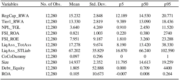
Table 2 presents the descriptive statistics of the study variables.

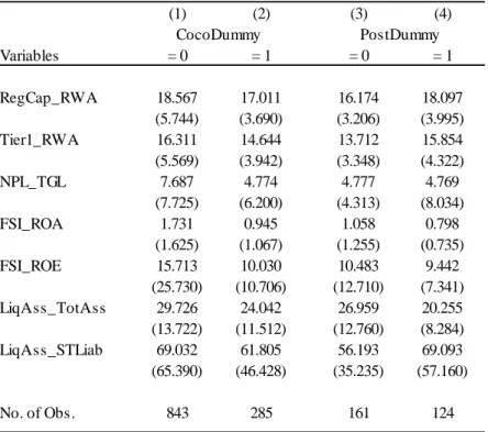
Looking in more detail, table 3 shows the summary statistics on country-level data. The comparison between columns 1 and 2 might suggest that riskier countries are more prone to allow the usage of CoCo bond as part of regulatory capital, since six out of seven indexes are worst in column 2. In addition, for the countries that have a bank that has issued CoCo bonds, a first analysis of the evolution from column 3 to column 4 indicates an improvement of the financial stability indexes.

[Insert Table 3 here]

3.2 EMPIRICAL STRATEGY

3.2.1 REGRESSION MODEL

To assess the effect of CoCo issuance on financial stability, I am first interested in estimating regressions on the form:

FinStabit = β0 + β1CoCoDummyit + β2Xit + αt + αi + εit (1)

where i indexes banks, t indexes time, CoCoDummyit is a dummy variable that equals one if bank issues a CoCo bond and zero elsewhere; Xit are controls variables; αt are year fixed effects; αi are bank fixed effects; and εit is the error term. I am particularly interested in the coefficient β1.

The dependent variables of the models I estimate (FinStabit) are some of the IMF’s Financial Soundness Indicators (FSIs), namely, Regulatory capital to risk-weighted assets - RegCap_RWA; Regulatory Tier 1 capital to risk-weighted assets - Tier1_RWA;

Nonperforming loans to total gross loans - NPL_TGL; Return on assets - FSI_ROA; Return on equity - FSI_ROE; Liquid assets to total assets - LiqAss_TotAss; and Liquid assets to short-term liabilities - LiqAss_STLiab. By choosing this selection, from regulatory capital and return, to nonperforming loans and liquidity, I aim to surround some areas of financial stability. The bank size (Size) is measured as the natural logarithm of total assets; capital structure (Debt_Equity) is the ratio between total debt and equity; and profitability (ROA) of the bank is calculated by the return on assets. If issuing CoCo bonds has a positive impact on financial stability, I expect all the coefficients to be positive, except for Nonperforming loans to total gross loans – NPL_TGL, which should be negative, meaning a reduction on nonperforming loans.

3.2.2 DIFFERENCES-IN-DIFFERENCES ESTIMATION

In this second analysis, I examine the effect of the impact of CoCo bond issuance on financial stability using essentially a differences-in-differences methodology. For the country-level data, the basic regression I estimate is:

FinStabit = α + β1*CoCoTreatit + β2*Controlit-1 + CountryFEi + YearFEt + εit (2)

where i indexes countries, t indexes time, FinStabit is the dependent variable of interest (the selected FSIs), CoCoTreatit is the interaction between variables CoCoDummyi and

PostDummyt, being CoCoDummyi a dummy variable that equals one if the country i has a bank that has issued CoCo bonds and zero elsewhere, PostDummyt a dummy variable that switches to one in the year that one of its bank has issued CoCo, staying one hereafter, and equals zero for all preceding years, and εi,t is an error term. The control variable used in this

regression is the logarithm of the lagged GDP per capita (ln_GDP_capita_lag1). All estimations control for country- and year- fixed effects. The coefficient of interest is β1, which captures the differential effect of the issuance in the financial stability index.

Following Bertrand and Mullainathan (2003), this approach can also be better understood with an example. Consider the United States of America for instance. Since the American regulator did not allow the usage of CoCo bonds as part of Tier 1 Capital, both USA’s CoCoDummyi and PostDummyt equals zero. German banks, on the other hand, can use CoCo bonds as regulatory capital, so Germany’s CoCoDummyi equals one. Moreover, Germany’s PostDummyt switches to 1 from 2014 on, since the first issuance of a German bank was on May 2014, and equals zero until 2013.

I acknowledge, however, that CoCo issuance is not a strict natural experiment due to the non-randomly selection of countries and banks. Looking again at the United States of America, one possible explanation for U.S. regulators choosing not to embrace CoCo in the same way as European and Asian regulators lays on CoCo’s interest tax-deductibility. Given that CoCos can have more favorable tax treatment than common equity, this may be more appealing for banks to issue CoCo instead of equity, going against the best interest of a country’s fiscal policy.

4 RESULTS

4.1 BASELINE REGRESSION

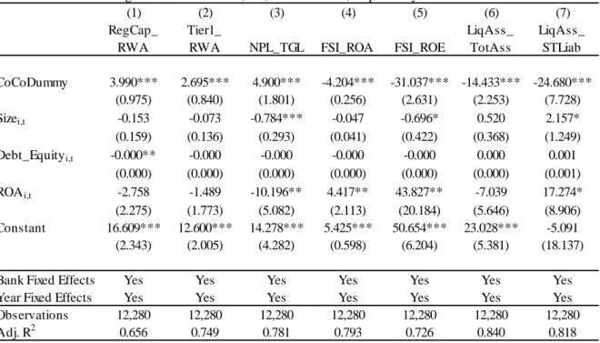
The results obtained from Eq. 1 appear in Table 4, which summarizes the empirical results for financial stability measures. As it was expected, since CoCo bond issuance has a direct impact on Regulatory Capital and on Tier 1 Capital, I find positive and significant

results for RegCap_RWA and Tier1_RWA (columns 1 and 2). Nevertheless, for the other five financial stability units, I find opposite results. The result for NPL_TGL shown in column 3 is positive and significant (4.9 bps), meaning that the issuance of CoCo bond increases the nonperforming loans to total gross loans ratio. While LiqAss_TotAss ratio dropped by 14.4 bps and LiqAss_STLiab dropped by 24.7 bps, FSI_ROA dropped by 4.2 bps and FSI_ROE dropped by a much-bigger 32.0 bps, which suggests that both banks’ returns and their liquidity are negatively affected by CoCo issuance. One possible scenario for the situation described above is that the money originated by the CoCo sale is being used to finance new and, to some extent, not so profitable projects, since it is possible to observe a negative impact on returns and liquidity. Echoing Admati et al. (2013), these findings may suggest that, instead of investing in these hybrid instruments, a better capitalized bank would suffer fewer distortions in lending decisions and could perform better.

[Insert Table 4 here]

Regarding the control variables, I highlight the following: (i) for the NPL_TGL dependent variable, both Size and ROA present a negative and significant impact, which could somehow imply that CoCo issuance by profitable and big banks is positive for nonperforming loans; (ii) both FSI_ROA and FSI_ROE show positive and significant result from ROA, being this result already expected, although the Size coefficient for FSI_ROE was negative and significant; (iii) last, for LiqAss_STLiab, results are shown to be positive and significant for both Size and ROA. This could also mean that CoCo issuance by profitable and big banks has a positive impact on liquidity.

4.2 DIFFERENCES-IN-DIFFERENCES ANALYSIS

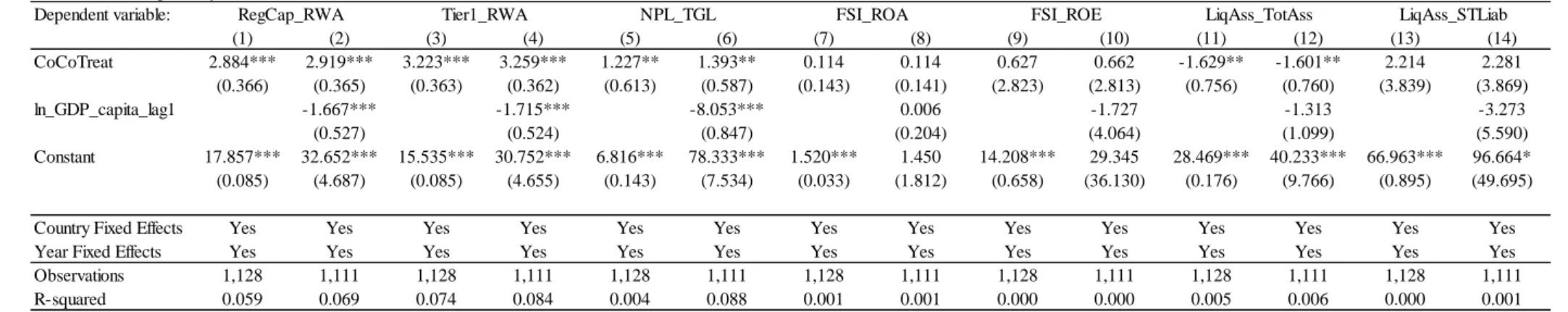
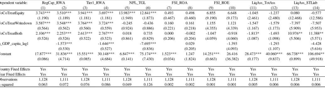
Table 5 presents the differences-in-differences regression results for the effects of CoCo issuance on the financial stability indexes. The odd columns show the results without controlling for lagged GDP per capita, and the even columns report the results considering this control. Columns 1 to 4 show positive and significant coefficients, meaning an improvement on stability. On the other hand, a positive and significant increase in the non performing loans ratio, columns 5 and 6, may suggest a problem on stability. Although one may expect a positive result for the liquid assets to total assets ratio, since the issuance of CoCo bond represents, initially, an increase in Cash and Cash Equivalents and in Total Assets, the negative and significant results found in columns 11 and 12 could also indicate a misusage of the cash raised from the issuance. Whilst the 1.4 bps increase in NPL ratio (column 6) and the 1.6 bps decrease in liquidity ratio (column 12) may not be economically large, these decreases should represent a warning sign to authorities. Regarding return on assets, return on equity and liquid assets to short-term liabilities indexes, columns 7 to 10 and 13 and 14, they show positive and non-significant results. It is noteworthy that more than 60% of the analyzed banks have issued CoCo bonds at least a second time. These results echo Fajardo and Mendes (2019), as they find that issuing CoCo bonds the first time decreases systemic risk as a positive response to a future crisis, but the second issuance increases the systemic risk, possibly by demonstrating a higher risk of financial distress or capital needs.

I acknowledge that a better control group would have been the countries in which the regulators allow the issuance of CoCo but the banks choose not to issue. However, to the best of my knowledge, there is no country in this situation, since every representative country that permitted CoCo bond, has at least one issuing bank.

5 ROBUSTNESS CHECKS

The set of tests presented so far have shown mixed results. Apart from the regulatory capital indexes, which showed positive and significant results, it is still not clear whether CoCo bonds have a positive impact on financial stability. In order to address potential concerns with empirical biases in the estimations, I perform a number of robustness tests and various further checks. The first robustness check considers the amount issued by banks as the major independent variable. Instead of only looking at whether a bank has issued CoCo or not, I analyze the impact of principal amount on the financial stability. The second robustness check refers to the two major classes of conversion mechanisms: conversion into common equity and principal write-down. For the conversion-into-equity CoCos, the conversion formula can be based either on the equity price on the day when the CoCo converts or on a pre-specified formula of number of shares for each bond, and even on some combination of the two. For principal write-down CoCos, the principal can be either fully or partially written off when the CoCo trigger is hit. Since it is a bank decision, and the bank can issue different CoCo bonds with different conversion mechanisms, there may be countries with both conversions. Taking into account that Europe (56%) and Asia (31%) represent 87% of total CoCo bond issued, my third analysis considers these two subsamples. I want to check for the effect on financial stability within these two continents. Last, I further conduct placebo tests to confirm that the conditions of the differences-in-differences are met.

In order to evaluate the effect of the amount issued on financial stability, I estimate the following regression:

FinStabit = β0 + β1LogAmountit + β2Xit + αt + αi + εit (3)

where LogAmountit is calculated as the natural logarithm of total amount issued by banks, and the other variables are previously described.

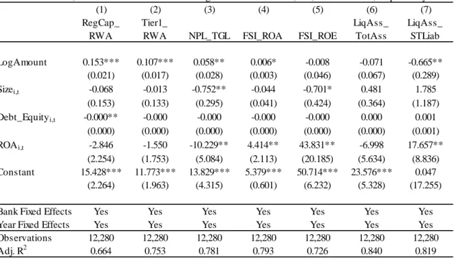
The results presented on Table 6 show expected positive and significant coefficients for RegCap_RWA and Tier1_RWA (columns 1 and 2). The coefficient for FSI_ROA (column 4) is also positive and significant, although not economically relevant. The positive and significant result for NPL_TGL (column 3) and negative and significant result for LiqAss_STLiab (column 7) indicate a negative effect: the more banks issue CoCo bonds, the less stable the financial system is.

[Insert Table 6 here]

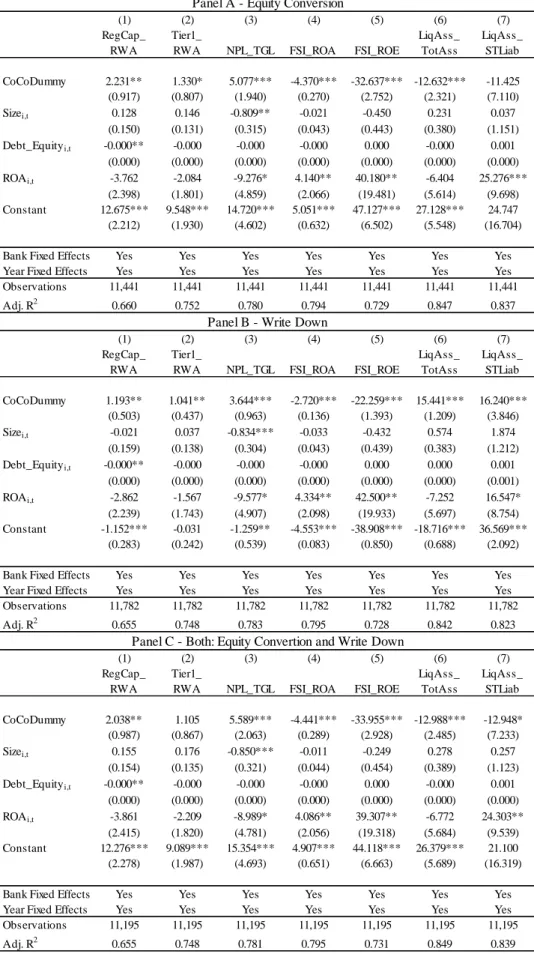
The second analysis refers to the two major classes of conversion mechanisms. Out of 1,509 banks analyzed, the 135 issuing banks can be divided into 40 with equity conversion, 79 with principal write-down, 12 with both and 4 non-specified. Four banks have no information whatsoever. As displayed in Table 7, there is no major difference between the main results and the results opened by conversion mechanisms. The only exception being the increase of 15.4 bps and 16.2 bps for liquidity indexes in the Write-down analysis, at columns 6 and 7. Following Avdjiev et al (2017) – they present that the impact on CDS spreads of CoCos that convert into equity is much stronger than the respective impact of principal

write-down CoCos –, I also find more prominent results for Equity Conversion in comparison with Write-Down, although the difference is not large.

[Insert Table 7 here]

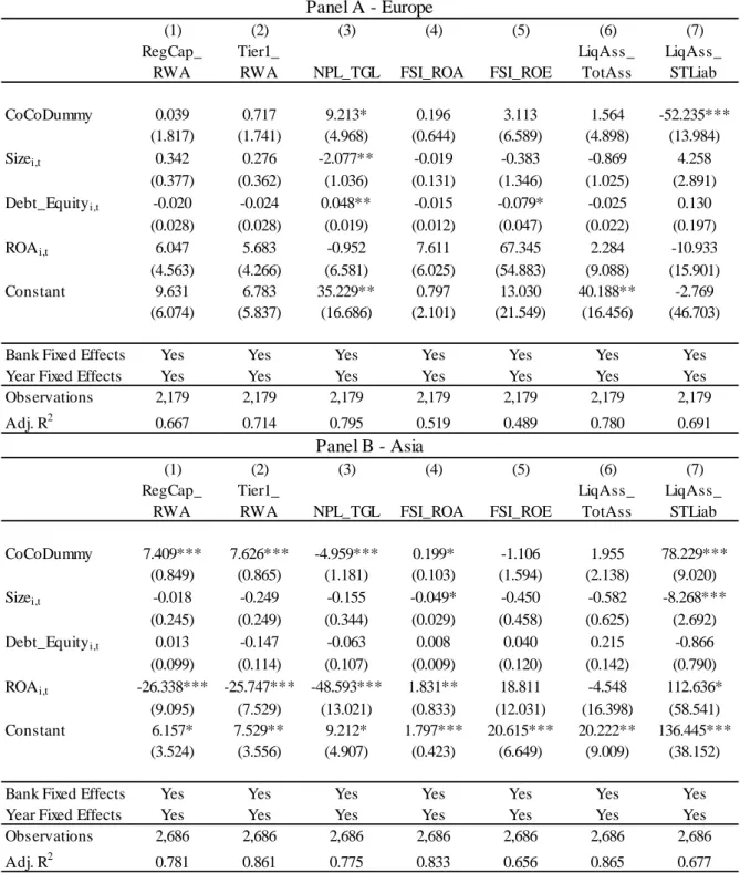
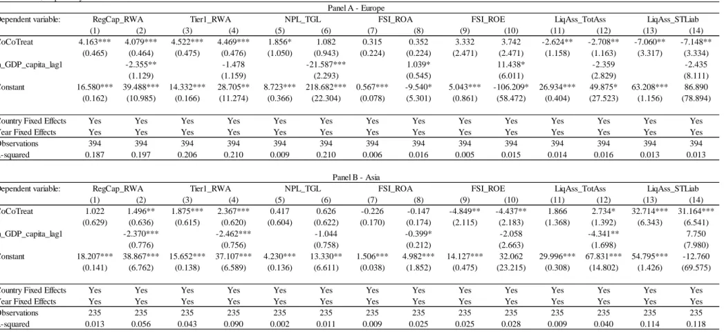
Table 8 illustrates results considering only Europe and Asia. The findings for Europe, nevertheless, are very peculiar when compared to the mains findings. One possible explanation for this scenario is that CoCo issuance plays no particular role when it comes to stabilizing the financial system in Europe. Even the regulatory capital indexes show no significant results.

The Asia’s coefficients, on the other hand, are even better than the main results: besides the positive and significant results for RegCap_RWA and Tier1_RWA (columns 1 and 2), the result for LiqAss_STLiab (column 7) is also positive and significant and the result for NPL_TGL (column 3) is negative and significant.

[Insert Table 8 here]

The 32 issuing countries are divided as follows: 2 with equity conversion, 15 with principal write-down and 15 with both. Table 9 reports the results.

[Insert Table 9 here]

The findings of Table 9 confirm my earlier results about the impact of CoCo issuance on the financial stability indexes. These effects have a significant economic impact and are

statistically similar to the ones reported using the full sample, confirming the robustness of the main results.

The diff-in-diff results for Europe, presented in Table 10 – Panel A, are in the same magnitude as of the main findings. The results for Asia (Table 10 – Panel B), on the other hand, was already expected. China accounts for 94% of Asian CoCo bond issuance and this constant and large issuance over the past years reflects new regulatory capital requirements and the associated replacement of subordinated debt. Since China’s banking system is mainly controlled by the four largest state-owned banks, it is no surprise to have found these results on China’s financial stability indexes.

[Insert Table 10 here]

Third, I further conduct placebo tests to confirm that the conditions of the differences-in-differences are met. I create two fictitious issuances that happen before the actual issuance and test whether the fictitious shocks influence the financial stability index of countries in treatment group in earlier years. In Placebo 1 analysis, I consider the year of issuance as of one year before the original one. Consider, for example, that a Chinese bank has first issued CoCo at October 2014, so China takes one from 2013 on for PostDummyt and zero until 2012. Similarly, in Placebo 2 analysis, I consider the year of issuance as of two years before the original one. I then re-estimate the baseline regressions in two separate samples covering different periods. Table 11 reports the results.

Although one might have expected the results to be statistically non-significant, meaning that the findings are mainly caused by the shock, the placebo results here are somehow divergent. Results as presented in Table 11 suggest an anticipation of the effect. The outcomes of the coefficient of RegCap_RWA from columns 2 of both Table 10 – Panel B (β = 2.469, p<0.01), Table 11 – Panel A (β = 2.553, p<0.01) and Table 4 (β = 2.919, p<0.01) exemplify that. While I argue that the issue of a CoCo bond is an exogenous shock, it may have taken some time between the country's authorization and the issuance of the bond, which in turn may have led to an anticipation of the effects.

6 CONCLUSION

The academic debate over CoCos has augmented after the financial crisis. As the CoCo issuance has enormously increased over the last decade, it urges among regulators and academia a better understanding of the potential impact of this hybrid security. My study provides novel evidence that suggests a mixed effect of CoCo issuance on financial stability. Through a panel analysis and a differences-in-differences identification strategy, I find positive and significant results for regulatory capital indexes, as it was expected, since CoCo bond issuance has a direct impact on Regulatory Capital and on Tier 1 Capital. Conversely, the coefficients for liquid assets to total assets ratio are negative and significant, meaning that the issuance of CoCo bonds is not good for financial stability.

In addition, I perform robustness checks, which confirm all the findings. Besides that, I acknowledge that a better control group would have been the countries in which the regulators allow the issuance of CoCo but the banks chose not to do so. However, to the best of my knowledge, there is no country in this situation, since every representative country that permitted CoCo bonds has at least one issuing bank. Lastly, although I argue that the

issuance of a CoCo bond is an exogenous shock, the results of the placebo analysis suggest an anticipation of the effect, as it may have taken some time between the country's authorization and the bond issuance.

7 REFERENCES

Acharya V., Pedersen L., Philippon T., and Richardson M., 2017. Measuring Systemic Risk. The Review of Financial Studies, 30 (1): 2–47

Admati A. R., DeMarzo P. M., Hellwig M. F., Pfleiderer P., 2013. Fallacies, Irrelevant Facts, and Myths in the Discussion of Capital Regulation: Why Bank Equity is Not Socially Expensive. Rock Center for Corporate Governance. Working Paper Series No 161 Adrian T. and Brunnermeier M. K., 2016. CoVaR. American Economic Review, 106 (7):

1705-41

Avdjiev S., Bogdanova B., Bolton P., Jiang W. and Kartasheva A., 2017. CoCo issuance and bank fragility. Bank for International Settlements Working Paper No 678

Avdjiev S., Bolton P., Jiang W., Kartasheva A. and Bogdanova B., 2015. CoCo Bond Issuance and Bank Funding Costs. Working Paper

Avdjiev S., Kartasheva A. and Bogdanova B., 2013. CoCos: a primer. Bank for International Settlements Quarterly Review, September 2013

Barclays, 2019. Prospectus Supplement to Prospectus dated April 6, 2018.

https://home.barclays/content/dam/home-barclays/documents/investor- relations/esma/capital-securities-documentation/tier-1-securities/contingent-tier- 1/Barclays%20PLC%20-%20USD%202bn%208%20per%20cent%20Fixed%20Rate%20Resetting%20Perpetual %20Subordinated%20Contingent%20Convertible%20Securities%20-%20ISM%20Admission%20Particulars.pdf

Basel Committee on Banking Supervision – BCBS, 2011. Basel III: International regulatory framework for banks. http://www.bis.org/bcbs/basel3.htm

Berg T. and Kaserer C., 2015. Does contingent capital induce excessive risk-taking? Journal of Financial Intermediation, 24 (2015) 356–385

Bertrand M. and Mullainathan S., 2003. Enjoying the Quiet Life? Corporate Governance and Managerial Preferences. Journal of Political Economy, vol. 111, no. 5, 2003

Bolton P. and Samama F., 2011. Capital access bonds: contingent capital with an option to convert. Economic Policy, p. 275–317, April 2011

Bonaparte Y., 2016. Global Financial Stability Index. Working Paper

Brave S. A. and Butters R., 2011. Monitoring Financial Stability: A Financial Conditions Index Approach. Economic Perspectives, Vol. 35, No. 1, p. 22, 2011

Brownlees C. and Engle R. F., 2017. SRISK: A Conditional Capital Shortfall Measure of Systemic Risk. The Review of Financial Studies, 30 (1): 48-79

Central Bank of Brazil, 2019. Financial Stability Report, Volume 18, Issue No. 1, April 2019 Deutsche Bank, 2014. Deutsche Bank Additional Tier 1 Notes 2014 Prospectus.

https://www.db.com/ir/en/download/DB_ISIN_DE000DB7XHP3_and_ISIN_XS10715 51474.pdf

Deutsche Bundesbank, 2018. Financial Stability Review, 2018

European Central Bank, 2018. Financial Stability Review, November 2018 Fajardo J. and Mendes L., 2019. CoCo Bonds and Systemic Risk. Working Paper

Fajardo J. and Mendes L., 2017. On the Propensity to Issue Contingent Convertible (CoCo) Bonds. Working Paper

Federal Reserve System. https://www.federalreserve.gov/financial-stability.htm

Ferreira C., Jenkinson N. and Wilson C., 2019. From Basel I to Basel III: Sequencing Implementation in Developing Economies. IMF Working Paper WP/19/127

Flannery M., 2014. Contingent Capital Instruments for Large Financial Institutions: A Review of the Literature. Annual Review of Financial Economics, vol. 6, issue 1, 225-240, 2014

Greene R. W., 2016. Understanding CoCos: What Operational Concerns & Global Trends Mean for U.S. Policymakers. M-RCBG Associate Working Paper Series No. 62

International Monetary Fund – IMF, 2006. Financial Soundness Indicators: Compilation Guide. Washington, DC

International Monetary Fund – IMF, 2019. Global Financial Stability Report: Lower for Longer. Washington, DC. October 2019.

Koziol C. and Lawrenz J., 2012. Contingent convertibles. Solving or seeding the next banking crisis? Journal of Banking & Finance 36, pp. 90–104, 2012

Martynova N. and Perotti E., 2018. Convertible bonds and bank risk-taking. Deutsche Bundesbank Discussion Paper No. 24/2018

Navajas M. C., and Thegeya A., 2013. Financial Soundness Indicators and Banking Crises. IMF Working Paper WP/13/263

Theil H., 1971. Principles of Econometrics. New York: John Wiley and Sons.

World Bank, 2016.

TABLES

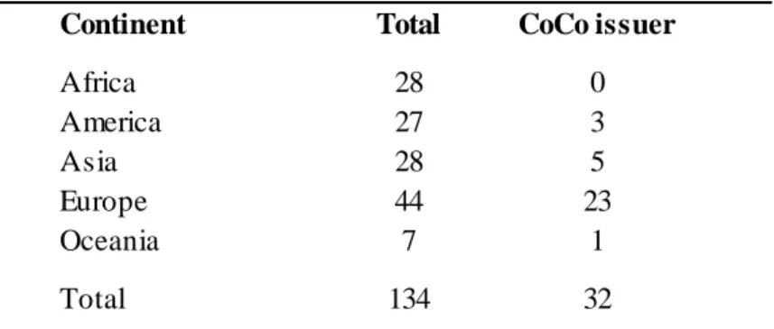
Table 1. Issuing Countries per Continent

Continent Total CoCo issuer

Africa 28 0 America 27 3 Asia 28 5 Europe 44 23 Oceania 7 1 Total 134 32

This table reports the number of countries of my samples, with the column Total representing the number of countries per continent analyzed and the column CoCo issuer representig the countries with bank issuing CoCo (America: Brazil, Colombia, M exico; Asia: China, India, Indonesia, Israel, M alaysia; Europe: Austria, Belgium, Croatia, Cyprus, Czech, Denmark, Estonia, Finland, France, Georgia,

Germany, Hungary, Italy, Luxembourg, Netherlands, Norway, Portugal, Slovak, Spain, Sweden, Switzerland, Turkey, UK; Oceania: Australia).

Table 2. Sample Descriptive Statistics

Panel A - Regression Approach

Variables No. of Obs. Mean Std. Dev. p5 p50 p95

RegCap_RWA 12,280 15.232 2.848 12.189 14.530 20.771 Tier1_RWA 12,280 13.330 2.819 9.389 13.090 18.436 NPL_TGL 12,280 3.640 4.269 0.910 2.450 11.520 FSI_ROA 12,280 0.821 1.003 0.220 0.380 2740 FSI_ROE 12,280 7.951 9.187 1.810 3.260 23.288 LiqAss_TotAss 12,280 17.278 9.674 8.190 13.420 38.330 LiqAss_STLiab 12,280 67.202 35.829 16.870 66.240 102.590 CoCoDummy 12,280 0.097 0.296 0 0 1 Size 12,280 14.937 2.352 11.795 14.613 19.259 Debt_Equity 12,280 1.805 52.888 0.000 0.709 4400 ROA 12,280 0.105 10.673 -0.007 0.008 0.264 Panel B - Difference-in-Difference

Variables No. of Obs. Mean Std. Dev. p5 p50 p95

RegCap_RWA 1,128 18.174 5.366 12.070 17.065 28.990 Tier1_RWA 1,128 15.890 5.254 9.530 14.650 26.800 NPL_TGL 1,128 6.951 7.475 0.850 4.220 20.130 FSI_ROA 1,128 1.532 1.542 -0.330 1.405 3.910 FSI_ROE 1,128 14.277 23.013 -3.220 14.060 32.000 LiqAss_TotAss 1,128 28.290 13.423 10.940 25.495 56.490 LiqAss_STLiab 1,128 67.206 61.217 19.700 47.500 170.650 CoCoDummy 1,128 0.253 0.437 0 0 1 ln_GDP_capita_lag1 1,111 8.891 1.383 6.509 8.923 10.955 This table reports descriptive statistics of my samples. Panel A sample covers the period from 2010 to 2018 and Panel B sample covers the period from 2008 to 2018. All variables are described in the text. I report the means, standard deviations, 5th percentiles, 50th percentiles, 95th percentiles, and the number of observations.

Table 3. Summary Statistics (Country-Level Data) (1) (2) (3) (4) CocoDummy PostDummy Variables = 0 = 1 = 0 = 1 RegCap_RWA 18.567 17.011 16.174 18.097 (5.744) (3.690) (3.206) (3.995) Tier1_RWA 16.311 14.644 13.712 15.854 (5.569) (3.942) (3.348) (4.322) NPL_TGL 7.687 4.774 4.777 4.769 (7.725) (6.200) (4.313) (8.034) FSI_ROA 1.731 0.945 1.058 0.798 (1.625) (1.067) (1.255) (0.735) FSI_ROE 15.713 10.030 10.483 9.442 (25.730) (10.706) (12.710) (7.341) LiqAss_TotAss 29.726 24.042 26.959 20.255 (13.722) (11.512) (12.760) (8.284) LiqAss_STLiab 69.032 61.805 56.193 69.093 (65.390) (46.428) (35.235) (57.160) No. of Obs. 843 285 161 124

This table reports means and standard deviations (in parentheses) on country-level data from 2009 to 2018. All variables are described in the text. Column (1) refers to countries that has not a bank that has issued CoCo bonds and Column (2) refers to countries that have a bank that has issued CoCo bonds. Columns (3) and (4) are subsets of Column (2): the former refers to the years before the issuance of CoCo, and the later refers to the year that one of its bank has issued CoCo and the years after the issuance.

Table 4. Baseline Regressions

(1) (2) (3) (4) (5) (6) (7)

RegCap_ RWA

Tier1_

RWA NPL_TGL FSI_ROA FSI_ROE

LiqAss_ TotAss LiqAss_ STLiab CoCoDummy 3.990*** 2.695*** 4.900*** -4.204*** -31.037*** -14.433*** -24.680*** (0.975) (0.840) (1.801) (0.256) (2.631) (2.253) (7.728) Sizei,t -0.153 -0.073 -0.784*** -0.047 -0.696* 0.520 2.157* (0.159) (0.136) (0.293) (0.041) (0.422) (0.368) (1.249) Debt_Equityi,t -0.000** -0.000 -0.000 -0.000 -0.000 0.000 0.001 (0.000) (0.000) (0.000) (0.000) (0.000) (0.000) (0.001) ROAi,t -2.758 -1.489 -10.196** 4.417** 43.827** -7.039 17.274* (2.275) (1.773) (5.082) (2.113) (20.184) (5.646) (8.906) Constant 16.609*** 12.600*** 14.278*** 5.425*** 50.654*** 23.028*** -5.091 (2.343) (2.005) (4.282) (0.598) (6.204) (5.381) (18.137)

Bank Fixed Effects Yes Yes Yes Yes Yes Yes Yes

Year Fixed Effects Yes Yes Yes Yes Yes Yes Yes

Observations 12,280 12,280 12,280 12,280 12,280 12,280 12,280

Adj. R2 0.656 0.749 0.781 0.793 0.726 0.840 0.818

This table presents the baseline regression results for the impact of CoCo issuance on the financial stability indexes. The analysis is based on annually data covering the period from 2010 to 2018. All variables are described in the text. Robust standard errors clustered at bank level are shown in parentheses and *, ** and *** denote statistical significance at the 10%, 5%, and 1% levels, respectively.

Table 5. The impact of CoCo issuance on the financial stability indexes

Dependent variable: RegCap_RWA Tier1_RWA NPL_TGL FSI_ROA FSI_ROE LiqAss_TotAss LiqAss_STLiab

(1) (2) (3) (4) (5) (6) (7) (8) (9) (10) (11) (12) (13) (14) CoCoTreat 2.884*** 2.919*** 3.223*** 3.259*** 1.227** 1.393** 0.114 0.114 0.627 0.662 -1.629** -1.601** 2.214 2.281 (0.366) (0.365) (0.363) (0.362) (0.613) (0.587) (0.143) (0.141) (2.823) (2.813) (0.756) (0.760) (3.839) (3.869) ln_GDP_capita_lag1 -1.667*** -1.715*** -8.053*** 0.006 -1.727 -1.313 -3.273 (0.527) (0.524) (0.847) (0.204) (4.064) (1.099) (5.590) Constant 17.857*** 32.652*** 15.535*** 30.752*** 6.816*** 78.333*** 1.520*** 1.450 14.208*** 29.345 28.469*** 40.233*** 66.963*** 96.664* (0.085) (4.687) (0.085) (4.655) (0.143) (7.534) (0.033) (1.812) (0.658) (36.130) (0.176) (9.766) (0.895) (49.695)

Country Fixed Effects Yes Yes Yes Yes Yes Yes Yes Yes Yes Yes Yes Yes Yes Yes

Year Fixed Effects Yes Yes Yes Yes Yes Yes Yes Yes Yes Yes Yes Yes Yes Yes

Observations 1,128 1,111 1,128 1,111 1,128 1,111 1,128 1,111 1,128 1,111 1,128 1,111 1,128 1,111

R-squared 0.059 0.069 0.074 0.084 0.004 0.088 0.001 0.001 0.000 0.000 0.005 0.006 0.000 0.001

This table presents OLS regression results for the impact of CoCo issuance on the financial stability indexes. I control for lagged country characteristics, country fixed effects, and year fixed effects in all regressions. The analysis is based on annually data covering the period from 2009 to 2018. All variables are described in the text. Standard errors are shown in parentheses and *, ** and *** denote statistical significance at the 10%, 5%, and 1% levels, respectively.

Table 6. Baseline Regressions by amount issued

(1) (2) (3) (4) (5) (6) (7)

RegCap_ RWA

Tier1_

RWA NPL_TGL FSI_ROA FSI_ROE

LiqAss_ TotAss LiqAss_ STLiab LogAmount 0.153*** 0.107*** 0.058** 0.006* -0.008 -0.071 -0.665** (0.021) (0.017) (0.028) (0.003) (0.046) (0.067) (0.289) Sizei,t -0.068 -0.013 -0.752** -0.044 -0.701* 0.481 1.785 (0.153) (0.133) (0.295) (0.041) (0.424) (0.364) (1.187) Debt_Equityi,t -0.000** -0.000 -0.000 -0.000 -0.000 0.000 0.001 (0.000) (0.000) (0.000) (0.000) (0.000) (0.000) (0.001) ROAi,t -2.846 -1.550 -10.229** 4.414** 43.831** -6.998 17.657** (2.254) (1.753) (5.084) (2.113) (20.185) (5.634) (8.836) Constant 15.428*** 11.773*** 13.829*** 5.379*** 50.714*** 23.576*** 0.047 (2.264) (1.963) (4.315) (0.601) (6.232) (5.328) (17.255)

Bank Fixed Effects Yes Yes Yes Yes Yes Yes Yes

Year Fixed Effects Yes Yes Yes Yes Yes Yes Yes

Observations 12,280 12,280 12,280 12,280 12,280 12,280 12,280

Adj. R2 0.664 0.753 0.781 0.793 0.726 0.840 0.819

This table presents the regression results for the impact of CoCo issuance on the financial stability indexes, considering the amount issued. The analysis is based on annually data covering the period from 2010 to 2018. All variables are described in the text. Robust standard errors clustered at bank level are shown in