Acoustic oceanographic buoy data report Makai Ex 2005

(1)

CINTAL - Centro de Investiga¸

c˜

ao Tecnol´

ogica do Algarve

Universidade do Algarve

Acoustic Oceanographic Buoy Data Report

Makai Ex 2005

S.M. Jesus, A. Silva and F. Zabel

Rep 04/05 - SiPLAB 17/Nov/2005

University of Algarve tel: +351-289800131 Campus de Gambelas fax: +351-289864258 8005-139, Faro cintal@ualg.pt Portugal www.ualg.pt/cintal

(2)

Work requested by CINTAL

Universidade do Algarve, Campus de Gambelas, 8005-139 Faro, Portugal

tel/fax: +351-289864258

cintal@ualg.pt, www.ualg.pt/cintal Laboratory performing SiPLAB - Signal Processing Laboratory

the work Universidade do Algarve, FCT, Campus de Gambelas, 8005-139 Faro, Portugal

tel: +351-289800949, fax: +351-289819403 info@siplab.uceh.ualg.pt, www.ualg.pt/siplab Projects FCT projects NUACE - POSI/CPS/47824/2002,

RADAR (POCTI/CTA/47719/2002) and HFi-JRP

Title Makai Ex 2005 - Acoustic Oceanographic Buoy Data Report Authors S.M.Jesus, A.Silva, F. Zabel

Date November 17, 2005

Reference 04/05 - SiPLAB Number of pages 48 (fourty eight)

Abstract This report describes the data acquired with the

second version of the Acoustic Oceanographic Buoy (AOB2) during the Makai Ex 2005, that took place aboard the R/V Kilo Moana from September 15 to 27 2005, off the west coast of Kauai I. in Hawai, United States.

Clearance level UNCLASSIFIED

Distribution list HLS (1), NURC (1), NRL (1), UDEL(1), SPAWAR (1) SiPLAB(2), CINTAL (1)

Total number of copies 8 (eight)

Copyright Cintal@2005

Approved for publication

E. Alte da Veiga

(3)

III

Foreword and Acknowledgment

This report presents the testing of the most recent version of the Acoustic Oceanographic Buoy (AOB) system and the results obtained during the Makai Ex sea trial. The MakaiEx sea trial took place off the west coast of Kauai I., Hawaii, USA, in the period September 15 - 27, 2005.

The authors of this report would like to thank:

• all the personnel involved, including R/V Kilo Moana crew • the scientist in charge Michael B. Porter

• the University of Hawaii for its support

• FCT (Portugal) for the funding provided under projects NUACE (POSI/CPS/47824/ 2002) and RADAR (POCTI/CTA/47719/2002).

(4)

IV

(5)

List of Figures

2.1 Acoustic Oceanographic Buoy - version 2: receiving array and surface buoy structure (a) buoy at sea (b). . . 14 3.1 Makai Exeperiment site off the north west coast of Kauai I., Hawaii (US). 16 3.2 MakaiEX area multibeam survey (University of New Hampshire). . . 17 3.3 MakaiEX bathymetry map with thermistor string locations. . . 18 3.4 recorded XBT (blue)/XCTD (red) casts: temperature profiles (a), sound

velocity (b) and XBT location over the area bathymetry (c). . . 19 3.5 thermistor string temperature data recorded on TS2 (a) and TS5 (b). . . . 19 3.6 first three EOF’s computed from thermistor string TS2 data. . . 20 3.7 hull mount ADCP: absolute value of the u-East/West component (a) and

of the v-North/South component (b) in m/s. The blank portions denote regions where there is no data . . . 21 3.8 GPS estimated AOB2 drifts during days 261 to 266. . . 22 3.9 GPS estimated AOB2 drift velocity for Drifts 1, 2, 3 and 4 in plots (a)

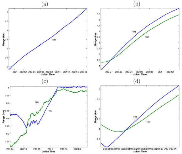
through (d) for days 261 to 266, respectively. . . 22 3.10 Source - receiver ranges as estimated from GPS for drifts 1, 2, 3, and 4

during days 261 to 266, respectively (a), (b), (c) and (d): from TB1 - blue line and from TB2 - green line; . . . 23 3.11 SPAWAR testbed mooring design (a) and prior to deployment (b). . . 24 3.12 GPS estimated AOB2 drift and KM track during day 268. . . 24 3.13 source - receiver ranges as estimated from GPS for drift 5 during day 268

for TB1 (blue) and TB2 (green) (a); source depth is constant for TB2 according to table 3.1 and for TB1 during the KM tow given in (b). . . 25 3.14 GPS estimated AOB2 drift 6, RHIB boat and KM tracks during day 269. . 25 3.15 source - receiver ranges as estimated from GPS for drift 6 during day 269. 26 4.1 LUBELL sources frequency response: model 916C3 (a) and model 1424HP

(b). . . 27 VII

(8)

VIII LIST OF FIGURES

4.2 structure of the each transmitted data block. . . 28 4.3 structure of the comomn probe used on each data block during the MakaiEx

sea trial, Probes and Comms phase. . . 29 4.4 spectrograms and relative power spectra for the transmitted probe signals

p ps (a), p lfm (b) and p pslfm (c). . . 30 4.5 drift1 received signal on hyd 3, at 55 m depth, start time JD262 00:14:42

UTC: UALg sequence as received from TB1 at approximately 2.2 km range to the North. . . 31 4.6 drift2 received signal on hydrophones 5 to 8, from depth 65 to 80 m, at start

time JD262 21:30:01 UTC: common probe followed by NRL1 sequence as received from TB1 at approximately 1 km range to the North. . . 33 4.7 UALG sequence received from testbed 2 on hyd 3, at 55 m depth, during

drift 3 at start time JD263 04:16:02 UTC. . . 33 4.8 drift5 received signal on hydrophone3 at 55 m depth, at start time JD267

23:15 UTC showing TB1 transmission ending and TB2 transmissions start-ing (a) and at JD267 23:27 UTC where durstart-ing WHOI time slot TB1 trans-mission superimposes on the signal received from TB2. . . 34 4.9 received signal on hydrophone3 at 55 m depth during drift 6: with small

Lubell source (model 916C3) at approximately 2.2 km range (a) and with large Lubell source (model 1424HP) during tow at approximately 1.5 km range. . . 35 4.10 pulse compressed common probe LFMs for hydrophone 6 (70 m depth) at

JD262 21:31:01 UTC of figure 4.6. . . 36 4.11 leading edge aligned mean LFM correlations (a) and envelopes (b) over

sensor depth for the common probe of figure 4.9 at time JD262 21:31:01 UTC. . . 36 4.12 PPC time focus structure of the common probe received signals by using the

(9)

Abstract

It is now well accepted in the underwater acoustic scientific community that below, say, 1 kHz acoustic propagation models are accurate enough to be able to predict the received acoustic field up to the point of allowing precise and reliable source tracking in range and depth with only limited environmental information. This results from a large number of studies both theoretical and with real data, carried out in the last 20 years. With the event of underwater communications and the necessity to increase the signal bandwidth for allowing higher communication rates, the frequency band of interest was raised to above 10 kHz. In this frequency band the detailed knowledge of the environment - acoustic signal interplay is reduced. The purpose of the MakaiEx sea trial is to acquire data in a complete range of frequencies from 500 Hz up to 50 kHz, for a variety of applications ranging from high-frequency tomography, coherent SISO and MIMO applications, vector - sensor, active and passive sonar, etc...The MakaiEx sea trial, that took place off Kauai I. from 15 September - 2 October, involved a large number of teams both from government and international laboratories, universities and private companies, from various countries. Each team focused on its specific set of objectives in relation with its equipment or scientific interest. The team from the University of Algarve (UALg) focused on the data acquired by their receiving Acoustic Oceanographic Buoy - version 2 (AOB2) during six deployments in the period 15 - 27 September. This report describes the AOB2 data set as well as all the related environmental and geometrical data relative to the AOB2 deployments. The material described herein represents a valuable data set for supporting the research objectives of projects NUACE1_{, namely to fulfill NUACE’s task 3 and 4 and}

RADAR2_{, namely its tasks 2 and 3 devoted to the developement and testing of a field of}

sonobuoys.

1_{Non-cooperative Underwater Acoustic Channel Estimation, FCT contract POSI/CPS/47824/2002,}

initiated in January 2004.

2_{Environmental} _Assessment _with _a _Random _Array _of _Acoustic _Receivers, _FCT _contract

POCTI/CTA/47719/2002, initiated in October 2004.

(10)

10 LIST OF FIGURES

(11)

Chapter 1 Introduction

Twenty years ago, matched-field processing (MFP) application on real data was made possible due to, at the time, recent developments on acoustic propagation codes and ad-vances in computer power. In those days, MFP was seen as a rather ambitious technique strongly dependent on the correct reproduction of the acoustic field both in amplitude and phase using a computer model initialized with field recorded environmental and geo-metric data. In most cases imprecise knowledge of environmental or geogeo-metric quantites, often prevented MFP to obtain a sustained source location estimate through time. The knowledge about signal propagation modelling, signal processing and optimization evolved so dramatically that, nowadays, it is scientifically admited that it is possible to track a sound source in range and depth almost in any environment with only a crude knowledge of the environment itself[1, 2]. Strangely enough most MFP studies were limited to the frequency range below 2 kHz. The reason for this is that geometry uncertainties were strongly dependent on signals wavelength, which would make it (probably) impossible to use at higher frequencies. More recently, the work of Hursky [3] has shown that it is indeed possible to pursue the MFP approach at higher frequencies, provided that the signal bandwidth is sufficient and that the transmitted signal is known at the receiver (which might be a drawback for some applications). This, and other similar studies, have triggered an increasing interest on high frequency (HF) environmental acoustics. Long standing problems in HF acoustics such as site and time dependent dropouts observed in coherent underwater communications (UCOMs), underwater tracking and positioning and accurate acoustic propagation modelling, are legitimate issues that deserve the attention of the scientific community.

The High-Frequency initiative (HFi) took off from a white paper on the subject, pre-pared by M. Porter in September 2003, that outlined a number of relevant issues on this field, setting pace for the research in this area with a 10 year horizon. This effort involves a wide spectrum of objectives that reflect specific interests such as: high-resolution to-mography, acoustic propagation modelling in the high frequency range, understanding of the acoustic - environment interaction at high frequencies and its influence on underwater communications among others. The MakaiEx sea trial was the third experiment specif-ically planned to acquire data to support HFi. The MakaiEx sea trial test plan1 _{lists a}

much broader range of objectives, including technical testing of numerous equipment and specific issues of scientific interest to particular teams involved in the experiment.

The SiPLAB team is part of the HFi with a particular interest on the usage of

environ-1_document _{ExperimentPlan Rev19.ppt} _can _be _obtained _from _the _MakaiEx _web _site

www.hlsresearch.com/Makai (password protected).

(12)

12 CHAPTER 1. INTRODUCTION

mental knowledge for underwater acoustic communications as relevant for fullfiling and supporting tasks 3 and 4 of project NUACE (POSI/CPS/47824/2002) and for equipment testing under task 2 and 3 of project RADAR (POCTI/CTA/47719/2002). Projects NU-ACE and RADAR were awarded by the coordinating institution CINTAL to SiPLAB for material execution. In particular, acquiring acoustic data in a frequency band well above the ULVA allowed band 0 - 2 kHz is important for project NUACE. This topic nicely interfaces with the development of the AOB system being pursued under task 2 of project RADAR.

The present document makes a complete report of the various data sets acquired dur-ing the MakaiEx sea trial between Sep 15 - 27 both acoustic and non-acoustic, as well as, accompanying data such as ship’s and buoy’s position, currents, temperature pro-files, geo-acoustic information and other concurrent remote sensing data. The companion DVD-ROM set contains all the basic data and respective master routines for data manip-ulation and pre-processing. This report is organized as follows: chapter 2 makes a short description of the AOB2 both from the hardware and software perspectives; chapter 3 describes the sea trial itself with various archival data sets, bathymetry, geometries and environment information recorded during the experiment; chapter 4 describes the acoustic data captured by the AOB2 system as well as all relevant information regarding signal transmission and preliminary results on the received data. Finally chapter 5 concludes this report giving some hints about most interesting sets for posterior processing. Sev-eral annexes with complete listings of data sets and other complementary information complete this report.

(13)

Chapter 2 The Acoustic Oceanographic Buoy

-version 2 (AOB2)

The AOB concept started in 2002, during the LOCAPASS project1_{, where a preliminary}

version of the AOB was developed (see AOB1 report [4]) for more details). That first AOB version 1 was tested during the Maritime Rapid Environmental Assessment (MREA) sea trials in 2003 off the Italian coast, north of Elba I. [5] and in 2004 off the portuguese coast, approximately 50 km south from Lisbon [6].

The AOB2 hardware and software system will be described in a companion report, while here only a brief description is made, in relation with the necessary characteristics for data processing.

2.1 AOB2 hardware

The AOB2 is a light acoustic receiving device that incorporates last generation technology for acquiring, storing and processing acoustic and non-acoustic signals received in various channels along a vertical line array. The physical characteristics of the AOB2, in terms of size, weight and autonomy, will tend to those of a standard sonobuoy with, however, the capability of local data storage, processing and online data transmission. Data trans-mission is ensured by seamless integration into a wireless lan network, which allows for network tomography within ranges up to 10/20 kms. In this second AOB prototype sev-eral capabilities were improved relative to the first system tested in 2003/04, namely the buoy container and electronics / data acquisition. The container now has the dimensions and weight of a standard sonobuoy. Electronics and batteries are housed in two separate containers: the battery container houses a high performance Li-ion 15V / 48Ah, capable of driving the AOB2 during more than 12 hours and weighting only 4.5 Kg; the electronics container receives a PC104+ stack with both comercial off the shelf (COTS) boards and proprietary boards specifically designed for the AOB2. The electronics stack also has a OEM GPS and a wlan amplifier for communications with the base station. The details of the electronics and mechanics parts are left for a future report and only the receiving hydrophone array and data acquisition characteristics are described below, due to their

1_{Passive source localization with a random network of acoustic buoys in shallow water (LOCAPASS),}

funded by the Foundation of Portuguese Universities and the Ministery of Defence.

(14)

14CHAPTER 2. THE ACOUSTIC OCEANOGRAPHIC BUOY - VERSION 2 (AOB2)

impact for the data processing.

2.2 AOB2 receiving array

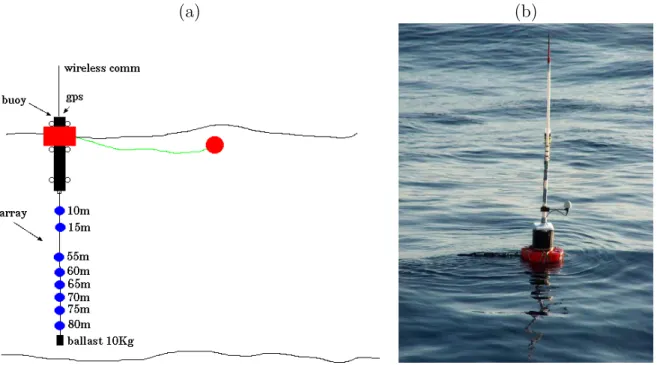
The hydrophone array is that of the AOB1 and is a light system composed of dedicated balanced twisted pairs for each hydrophone and a common power line attached to a 5 mm kevlar rope enveloped in a air fairing sleeve to maintain all wires together (see figure 2.1(a)). This system has a reduced water drag and allows for easy field maintenance when and if necessary. After the first deployment (see the buoy at sea during MakaiEx in 2.1(b)) a set of bungees was added between the top most attach point of the array and the bottom of the buoy container, in order to allow some surface wave decoupling of the vertical hydrophone array. The array has 8 hydrophones oddly distributed in the

(a) (b)

Figure 2.1: Acoustic Oceanographic Buoy - version 2: receiving array and surface buoy structure (a) buoy at sea (b).

70 m total acoustic aperture, at depths of: 10, 15, 55, 60, 65, 70, 75 and 80 m. The ensemble hydrophone - pre-amplifier were manufactured by Sensor Technology (Canada). The hydrophone sensitivity is -193.5 ± 1 dBV re 1 µPa 20◦ C for both broadside and endfire up to 18 kHz and with a flat frequency response from 1 Hz up to 28 kHz.

The pre-amplifier is a low noise differential amplifier that has a constant gain of 40 dB in the whole frequency band of interest between 10 Hz up to 50 kHz. Its noise has been measured to be smaller than 20 nV/√Hz. As it will be seen during the deployments, the pre-amplifier gain was often insufficient to fulfil the analogue to digital converter (ADC) ±5 V sensitivity at the frequencies used during the transmissions. This required some field tuning of the data acquisition in order to better use the dynamics of the ADC board.

(15)

2.3. AOB2 DATA ACQUISITION 15

2.3 AOB2 data acquisition

The data acquisition was performed by a dedicated ADC board attached to a DSP board. The ADC board itself is an LTC1864 from Linear Technology based on successive approx-imation with 16 bits, four modules and a total agregate frequency per module of 250kHz. The anti-aliasing filters are 8 pole low-pass analog Chebyshev implementations with a cutoff frequency of 16 kHz.

As explained above due to the pre-amplifier constant low gain of 40 dB when working in the high frequency range of the bandwidth, it was necessary to change the ADC sensitivity according to the source - receiver distance. The ADC has an internal variable gain setting leading to input sensitivities of ± 1, ± 2, ±5 and ± 10 volts. Sensitivity changes during the sea trial were as follows:

• Drift 1: dynamic range changed from ±5V to ±2V at 02:00 UTC • Drift 2: dynamic range set to ±5V during the whole run

• Drift 3: dynamic range changed from ±5V to ±2V at 04:00 UTC • Drift 4: dynamic range set to ±2V during the whole run

• Drift 5: dynamic range set to ±1V during the whole run

• Drift 6: dynamic range set to ±2V until 19:40 UTC, then changed to ±1V at 19:40 UTC and then to ±2V at 01:55 UTC.

The sampling frequency is derived from a high precision timer board that itself gets the synchro tops for its internal clock from the GPS 1PPS signal. So, one can say that the sampling interval was based on the Cesium clock of the GPS.

The Makai Ex sea trial served also as engineering test for new equipment, as was the case for the AOB2 surface buoy. In particular, as it will be seen below, a number of spikes across the whole frequency band well above the antialiasing cutoff frequency, were found during the first 3 deployments. This was found to be due to random bits flipping during data transmission between the DSP and the CPU, prior to archiving. This was found in all channels. After some bench testing it was found that temperature increase inside the container was responsible for this problem. Temperature monitoring inside the canister has shown that the temperature was steeply rising from 24 to 42◦C, during data acquisition. After strategically placing two micro fans the new temperature recording showed that dissipation through the highly heat conductive aluminium wall to maintain the inside temperature within 23 ◦C at all times.

A warning note should be made here regarding the convention used for converting actual calendar UTC date and time to UTC Julian time. In fact it is very useful to refer time at any moment of the sea trial by a single decimal common number like Julian time. One of the problems arises from the way this time is calculated for which there are two possible conventions: one is considering January 1st as day one or considering January 1st as day 0. In this data report and in agreement with the on board master clock the former has been used, so day September 15, 2005 02:00 local time will be coded as Julian time 258.5 UTC.

(16)

Chapter 3 The MakaiEx sea trial

3.1 Generalities and sea trial area

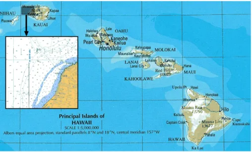
Figure 3.1: Makai Exeperiment site off the north west coast of Kauai I., Hawaii (US).

The selected area for the MakaiEx sea trial is shown in figure 3.1 while a detailed view of the slected area with bathymetry is shown in the insert. This is a well documented area since it is part of the Pacific Missile Range Facility (PMRF) of the US Navy, where a number of military exercises and acoustic experiments take place, in particular the Kauai Ex sea trial in 20031_{. The weather is generally calm dominated by North winds sometimes}

up to 20/30 knot and sea currents that offer a variable pattern but in general tend to circulate the Kauai I. shelf either towards NE or SSE. During the AOB2 testing the sea state was agitated during the first three first days with 3 m wave height and 35 knot of North wind, that then dropped to 10 knot wind and less than 0.5 m surface waves.

1_{KauaiEx password protected website from www.hlsresearch.com.}

(17)

3.2. GROUND TRUTH MEASUREMENTS 17

3.2 Ground truth measurements

3.2.1 Bottom data

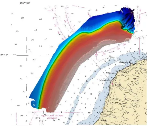
Extensive ground truth measurements were carried out in this area during previous exper-iments and showed that most of the bottom in the area is covered with coral sands over a basalt hard bottom. Coral sands are named after the desintegration of corals that cov-ered the bottom in the area. Previous grain size measurements and comparison with silica beach sand showed that sound velocity should be slightly higher in coral sands, approxi-mately 1700 to 1800 m/s. It is expected that coral sands cover most of the plateau around the Kauai I. and are washed down along the steep slopes. Sediment thickness is unknown but expected to be of a fraction of a meter to a few meters in most places according to previous sidescan surveys. In the last days of the sea trial, a sidescan/multibeam survey of the area took place using the KM hull mounted sonar system. A first image is shown in figure 3.2 where it can be seen an almost perfectly smooth and uniform area of constant depth around 80 - 100 m accompaining the island bathymetric contour, surrounded by the continental relatively steep slope to the deeper ocean to the West and to possibly softer bottoms to the shallower parts to the East. This data is under analysis at the University of New Hampshire, to be described in a separate report.

(18)

18 CHAPTER 3. THE MAKAIEX SEA TRIAL

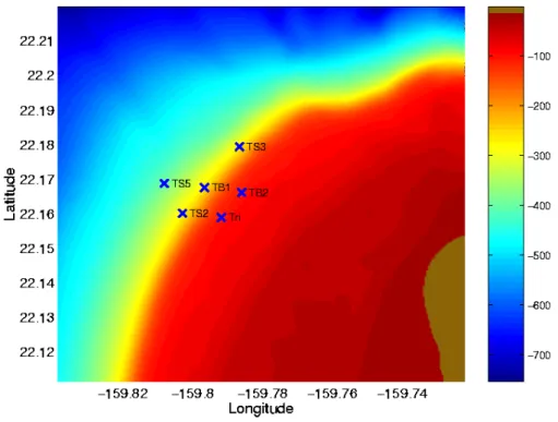
Figure 3.3: MakaiEX bathymetry map with thermistor string locations.

3.2.2 Water column data

XBT and XCTD casts

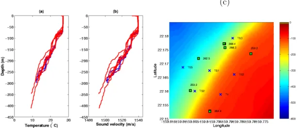
During MakaiEx a number of environmental recording equipment was deployed, in an attempt to collect as much environmental data as possible, mostly aiming at the water column variability. That included various thermistor strings, a waverider buoy and a bottom mounted ADCP. Whenever possible, CTDs, XBTs, XCTDs and current recordings with the KM hull mounted ADCP were made. However due to adverse weather conditions during the first deployments, four thermistor strings were lost (one was recovered but broken during deployment), as well as the waverider buoy and the bottom mounted ADCP. One of the other three thermistor strings could not be recovered. Eventually only two thermistor strings were successfuly deployed and recovered, which locations are shown in figure 3.3 together with a detailed bathymetry map of the sea trial area that will be used throughout this report. The actual measured temperature profiles obtained from XBT and XCTD casts and the calculated sound velocities are respectively shown in figure 3.4 (a) and (b), while plot (c) shows their location over the area bathymetry map.

Thermistor strings

Several thermistor strings were deployed but due to the adverse weather conditions en-countered during the first days of the sea trial, only the thermistor strings of stations 2b (TS2) and 3c (TS5) were recovered with successful data recordings. The data is shown in figure 3.5, TS2 in (a) and TS5 in (b). Since these moorings were using a sub-surface float to maintain the thermistor string straight up it is expected that the strong currents observed in the area might have tilted down the strings at least during part of the record-ings. For some unknown reason the depth sensors located in the upper sensor did not gave reliable results, but do show some oscillations over time. The data shown in figure

(19)

3.2. GROUND TRUTH MEASUREMENTS 19

(c)

Figure 3.4: recorded XBT (blue)/XCTD (red) casts: temperature profiles (a), sound ve-locity (b) and XBT location over the area bathymetry (c).

3.5 has not been corrected for the sub-surface depth sensor and the nominal depths of 20 m for TS2 and 16 m for TS5 were used. Since all the other sensor’s depth depend on the depth of the upper sensor, some possible depth shift in the whole readings is antici-pated. Strong internal tides can be clearly seen in the first three days of recording, where

Figure 3.5: thermistor string temperature data recorded on TS2 (a) and TS5 (b).

strong water column oscillations lead to almost the suppression of the thermocline in four consecutive days in TS2 (only 20 m thick). At the end of the recording there is a clear surface warming and extension of the thermocline reaching depths of nearly 100 m.

(20)

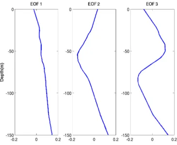
20 CHAPTER 3. THE MAKAIEX SEA TRIAL according to ˆ T (z) = ¯T + N X i=1 αiUi(z), 0 ≤ z ≤ H (3.1)

where αi are the EOF coefficients, Ui(z) the EOF’s and H is the water depth, chosen

equal to a minimum of 150 m in this example gave a set of EOF’s which first three are shown in figure 3.6 and are meant to represent more than 95% of the total energy in the water column. In order to obtain this decomposition the TS2 data were interpolated at every meter over the water column and extrapolated to the surface.

Figure 3.6: first three EOF’s computed from thermistor string TS2 data.

Current data

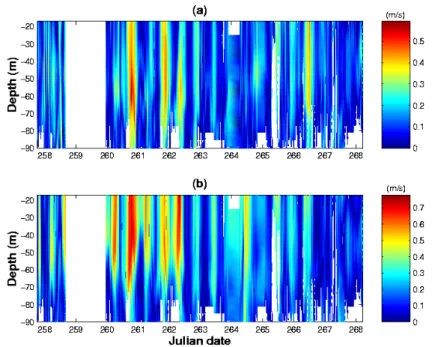
The Kilo Moana hull mounted ADCP was up and recording during most part of the cruise. Unfortunately it was shut off on the very first days in order to avoid interference with the reception of the SLIVA array, that was deployed starting from the second day on board (JD 259 18:47), in order to record some wind driven surface noise since the weather was quite rough (force 3 - 2/3 m wave height). In fact what appears from the ADCP recordings of figure 3.7 is that these very first cruise days were marked by very strong U, and specially V, currents of up to 0.8 m/s (1.6 kn). These days were full moon days which drove those currents and winds that highly influenced ship’s positioning for equipment deployment and moored gear that was being deployed. It is suspected that these environmental factors drove to the loss of thermistor TS1, and TS3 (broken during deployment) early on day 259 (late Sep 15) and TS1, the waverider buoy, the bottom ADCP and TS4 all deployed late on 259 and early 260 (afternoon Sep 16) and finally the loss of the ACDS system late on day 260 (morning of Sep 17). As it can be seen on figure 3.7, late day 260 early 261 correspond to the peak current of up to nearly 2 kn for which the ACDS mooring was clearly not prepared. During the rest of the cruise the observed currents are clearly lower with a single peak at 0.4 m/s on day 266, with much more equilibrated values between the u and v components which possibly explained the change of direction of the AOB2 drifts from up north on day 261 changing to northeast and then directly to east on the last deployments.

(21)

3.3. DEPLOYMENT GEOMETRIES 21

Figure 3.7: hull mount ADCP: absolute value of the u-East/West component (a) and of the v-North/South component (b) in m/s. The blank portions denote regions where there is no data

3.3 Deployment geometries

Most of the AOB2 deployments during MakaiEx where free drifting therefore, deployment geometries include AOB2 drifts 1, 2 and 4 in Julian days 261, 262 and 266 during which signals were being transmited from fixed bottom moored sources. AOB2 drifts 5 and 6 where KM or the RHIB boat were towing transmitting sources on Julian days 268 and 269. During day 263 the AOB2 was tethered at about 200 m from the stern of the KM that was approximately maintaining position. Although this deployment was not exactly a drift it was named as drift3.

3.3.1 AOB2 drifts 1 to 4

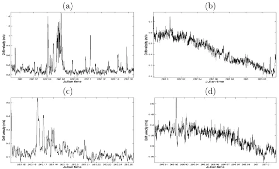
Figure 3.8 shows the first four AOB2 drifts together with the locations of the thermistors strings TS2, TS3 and TS5 as well as the locations of the fixed Testbed sources 1 and 2 and the receiving tripod from UDEL. During drift 3 the AOB2 was tethered to the KM. Figure 3.9 shows the velocity vector of the drift of the AOB2 during days 262 to 266. This figure clearly shows the AOB2 speed through the water, specially during drift 2 where it reached 0.6 m/s, i.e., over 1 kn and the AOB2 was almost lost since there was no wireless communication due to a system malfunction.

The data on figure 3.8 was used to calculate source - receiver ranges between TB1 / TB2 to the AOB2 as shown on figure 3.10. During Drift 1, only TB1 was deployed and therefore only the TB1 - AOB2 range is shown. TB2 was deployed during Drift 2 but was not turned on so there is are no TB2 transmissions during this run. One can remark the very “noisy” source range estimate during Drift 3, that was due to the fact that the AOB2 was tethered to KM that herself was on dynamic positioning at close range from TB1 and TB2. Plot (d) of figure 3.10 shows AOB2 range to both testbeds although there

(22)

22 CHAPTER 3. THE MAKAIEX SEA TRIAL

Figure 3.8: GPS estimated AOB2 drifts during days 261 to 266.

(a) (b)

(c) (d)

Figure 3.9: GPS estimated AOB2 drift velocity for Drifts 1, 2, 3 and 4 in plots (a) through (d) for days 261 to 266, respectively.

were no transmissions due to low battery power on testbeds.

The depths of the Testbeds were largely dependent on their location and on the exact design of the mooring. Each testbed was deployed twice but at the exact locations of the previous deployment as shown in table 3.1. The typical deployment design for the testbeds is shown in figure 3.11 where it can be remarked that the distance between the bottom and the transducer can vary by introducing a longer cable between the cement weight and the acoustic releasers. As it can be noticed in the before last column of table 3.1 that height from the bottom was increased from approximately 5 m in the first deployments to 13.5 m in the second deployments. Taking into acount those variables source depths are shown in the right most column of table 3.1.

(23)

(a) (b)

(c) (d)

Figure 3.10: Source - receiver ranges as estimated from GPS for drifts 1, 2, 3, and 4 during days 261 to 266, respectively (a), (b), (c) and (d): from TB1 - blue line and from TB2 - green line;

Deployment Lat Long Water depth Height SD (m) (m) (m) TB1 1 22.1674 -159.7976 215 4.8 210.2 TB1 2 22.1673 -159.7975 215 13.5 201.5 TB2 1 22.1660 -159.7869 103 4.8 98.2 TB2 2 22.1660 -159.7870 103 13.5 89.5

Table 3.1: locations and geometric characteristics of Testbeds; last column shows estimated source depth (m).

3.3.2 AOB2 drift 5

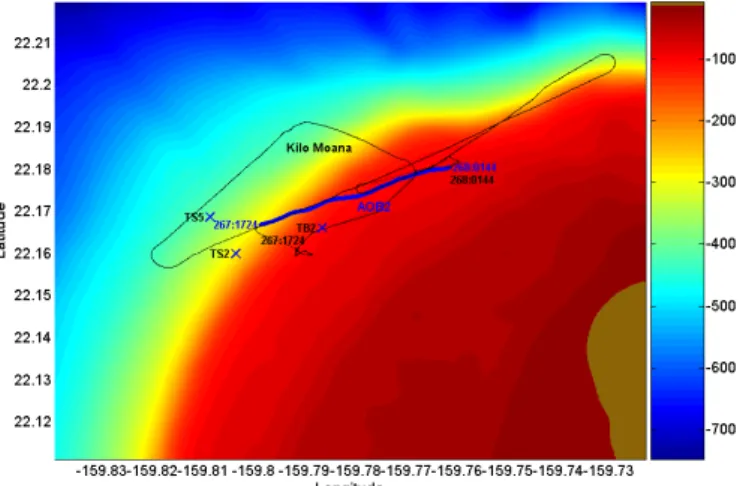
Figure 3.12 show the AOB2 drift together with the source tracks during day 268 (drift 5). On day 268 the transmitting source was TB1 mounted on a vertical towfish transmitting typical Testbed signals as specified in the “Probes and Comms” phase. TB2 was deployed at its usual location and transmitting. Note the complex pattern of KM that was supposed to allow for both range independent and range dependent propagation paths to the AOB2, by tracking along and across shore respectively. The AOB2, this time drifted nearly to the East, along a nicely range-independent area of approximately 100 m water depth.

(24)

24 CHAPTER 3. THE MAKAIEX SEA TRIAL (a) (b) (0.38m) strobe surface buoy grappling target 5−lb counter weight Threaded rod

Testbed transmitter battery cannister small shackle Subsurface flotation ’D’ ring ’D’ ring small shackle AT−408 modem transducer ITC−1007 8−16 kHz projector Concrete or equivalent (120# in water weight) Large shackle chain Swivel Testbed electronics cannister small shackle 1075’ (327 m) 34" (0.86) 36" (0.91 m) 32" (0.81 m) 12" (0.30 m) 15" (0.38 m) 7" (0.18 m) 28" (0.71 m) 30.5" (0.77 m) 4" (0.1 m) 15" 14.5" (0.37 m) 18.5" (0.47 m) 17 feet

Total weight in water = −33 lb

12" (0.308 m)

15.8 feet 4.826 m Testbed #1 Deployment #1, 9−17−05

Figure 3.11: SPAWAR testbed mooring design (a) and prior to deployment (b).

Figure 3.12: GPS estimated AOB2 drift and KM track during day 268.

TB2 (fixed - see position on table 3.1) and TB1 that was being towed by KM. Source depth during drift 5 was constant for TB2 as shown in table 3.1 and given in figure 3.13(b) for TB1 as given by a snapin depth(and temperature) recorder attached to the tow body.

3.3.3 AOB2 drift6

Day 269 was dedicated to “Field Calibration” operations and the LUBELL916C3 source was being towed by the RHIB boat in the morning and the large low frequency LUBELL

(25)

(a) (b)

Figure 3.13: source - receiver ranges as estimated from GPS for drift 5 during day 268 for TB1 (blue) and TB2 (green) (a); source depth is constant for TB2 according to table 3.1 and for TB1 during the KM tow given in (b).

1424HP source was being towed by KM in the afternoon. Respective tracks are shown in figure 3.14.

Figure 3.14: GPS estimated AOB2 drift 6, RHIB boat and KM tracks during day 269.

Figure 3.14 was also used to determine source receiver range between either RHIB boat or KM and the AOB2 for drift 6, as shown in figure 3.15(a). Black line was drawn from hand written GPS stations on the RHIB boat during the track; the green line was drawn from NURC portable GPS that was available during only the second North-South portion of the RHIB boat track and is, therefore, mostly superimposed on the hand written GPS stations (in black); red line was calculated from KM track that was towing the large Lubell 1424HP. Plot (b) of figure 3.15 shows recorded source depth for drift 6. Line colors black and red correspond to the small Lubell 916C3 and the large Lubell 1424HP tows, respectively.

(26)

in-26 CHAPTER 3. THE MAKAIEX SEA TRIAL

(a) (b)

Figure 3.15: source - receiver ranges as estimated from GPS for drift 6 during day 269.

formation obtained from the AOB2 gps log files (gps-deploy*.log where * runs from 1 to 6) and the actual source coordinates when testbeds where fixed and RHIB/KM gps logs when sources were under tow.

(27)

Chapter 4 Acoustic data

4.1 Emitted signals

4.1.1 Acoustic sources

Acoustic signals received by the AOB2 were emitted from a variety of sound sources that included the two testbeds 1 and 2 (TB1 and TB2) and the two LUBELL sources (LL916C3 and 1424HP). Some of these sources were fixed during the transmissions and some other were towed, as described in section 3.3. The frequency band of the transmitted signals was 8 - 14 kHz for the Testbeds and 500 - 14000 Hz for the LUBELL sources. Figure 4.1 shows the frequency responses of the two LUBELL sources: small LUBELL model 916C3 towed by the RHIB boat during first part of AOB2 drift6 in (a) and large LUBELL model 1424HP towed by KM during the second part of AOB2 drift 6 (b).

(a) (b)

Figure 4.1: LUBELL sources frequency response: model 916C3 (a) and model 1424HP (b).

(28)

28 CHAPTER 4. ACOUSTIC DATA

4.1.2 Transmitted sequences

There was a wide variety of signals transmitted during the MakaiEx sea trial that included two phases: the Probes and Comms (PC) phase and the Field Calibration (FC) phase. During the PC phase a transmissions schedule was used that allocated time slots to the various research teams on board and to the existing three transmitters. Unfortunately one of the transmitters was lost and therefore during approximately one third of the time no signals were transmitted. The transmission schedule is shown in table 4.1. On each hour, the first 30 minutes were dedicated to the single access signals and the second 30 minutes to the multi-access. Each 2 minutes data block has one probe signal, common to

Time(min) TB1 TB2 Time TB1 TB2

(min) (min)

0 blank blank 30 NRL1

2 HLS 32 NRL1

4 HLS 34 NRL1 NRL1

6 blank blank 36 blank blank

8 UDel 38 NRL2

10 UDel 40 NRL2

12 blank blank 42 NRL2 NRL2

14 UAlg 44 sil sil

16 UAlg 46 18 blank blank 48 20 WHOI1 50 22 WHOI1 52 24 blank blank 54 26 WHOI2 56 28 WHOI2 58

Table 4.1: transmit schedule of the ”Probes and Comms” phase: min 0 - 30 is the signal access phase while min 30 - 60 is the multiaccess phase.

all data blocks of all institutions, which structure is shown in the drawing of figure 4.2.

Figure 4.2: structure of the each transmitted data block.

The common probe

The common probe was designed by Thomas Folegot (NURC team), generated using the routine shown in appendix A.1 and is described in detail elsewhere. Here, only a generic description is given. The common probe has a total duration of 10 s and its overall strucuture is shown in figure 4.3. There are three sub regions: the first region is occupied by LFM upsweeps between 8 and 14 kHz with 50 ms time duration, during

(29)

4.1. EMITTED SIGNALS 29

4 s; the second region is occupied by a multitone signal, so called Comb signal, with 8 tones at various frequencies in the 8-14 kHz band with a duration of 2 s, and where each source has a specific set of frequencies, so the Combs of the common probes can be used to differentiate the transmitter; the third region contains a 4s-long M-sequence centered at 11 kHz with a 3000 chips/s bit rate. Each region is separated by a 200 ms blank space with no signal.

Figure 4.3: structure of the comomn probe used on each data block during the MakaiEx sea trial, Probes and Comms phase.

The UALg sequence

The UALg sequence was designed having in mind passive phase conjugation testing and is described in detail here. Each transmitted frame is composed of generic probe signals (PROBS) and data communications signals (COMMS). The COMMS signals are com-posed of three different types (SIG1, SIG2 and SIG3) and a 3 seconds silence (SIL) at the

end, in the following manner

SIG1 SIG1 SIG2 SIG2 SIG3 SIG3 SIL

17.7 s 17.7 s 17.9 s 17.9 s 17.9 s 17.9 s 3 s

with a total duration of 110 seconds. The SIGi signals are composed by probe signals

of different types and equal data signals. In SIG1 the probe signal, p ps, is the pulse

shape of the digital modulated data, in SIG2 the probe signal, p lfm, is a chirp that spans

the band of the digital modulated data, and in SIG3 the probe signal, p pslfm, is the

convolution of p lfm with p ps. Each probe signal is repeated several times before the data signal, and the data signal is composed of 15 repetitions of the same digital frame that we will call ’data’. So, each SIGi is composed as follows

SIG1

p ps SIL . . . p ps Sil data . . . data SIL 0.05 s 0.2 s . . . 0.05 s 0.2 s 1 s . . . 1 s 3 s

10x 15x 1x

SIG2

p lfm SIL . . . p lfm Sil data . . . data SIL 0.1 s 0.2 s . . . 0.1 s 0.2 s 1 s . . . 1 s 3 s

9x 15x 1x

(30)

p pslfm SIL . . . p pslfm Sil data . . . data SIL 0.1 s 0.2 s . . . 0.1 s 0.2 s 1 s . . . 1 s 3 s

9x 15x 1x

(a) (b) (c)

Figure 4.4: spectrograms and relative power spectra for the transmitted probe signals p ps (a), p lfm (b) and p pslfm (c).

The p ps signal is a root root raised cosine with 50% roll-off and a bandwidth of 3 kHz centered in the carrier frequency of 10 kHz; p lfm has a starting stop frequency of 8.5 kHz to 11.5 kHz and 90 ms effective duration; the p pslfm signal is the convolution of the previous two probe signals. All probe signals are shown in figure 4.4 for p ps, p lfm and p pslfm in (a), (b) and (c), respectively. The data signal is composed of 2000 symbols, where the first 127 are an M sequence and the others are generated randomly, they are BPSK modulated with a pulse shape equal to the p ps signal and a carrier frequency of 10 kHz.

The Field Calibration sequence

During the Field Calibration (FC) phase a different set of signals were transmitted both from the 916C3 Lubell and from the 1424HP Lubell sources, respectively towed from the RHIB boat and the KM. These sequences included short duration high frequency LFMs, M sequences in different bands and sum of tones across the whole band from 8 kHz down to 500 Hz. BPSK sequences were also transmitted both at low and high frequencies.

4.2 Received signals

4.2.1 Data format

The data, both acoustic and non acoustic, received on the AOB2 are stored on data files using a proprietary format that can be read using the routine ReadLOCAPASS.m shown in appendix A.2. This format can be summarized as follows:

• an ASCII header: cruise title, UTC GPS date and time of first sample on file, Lat - Lon GPS position, characteristics of non-acoustic and acoustic data such as sampling frequency, number of channels, sample size and total number of samples • non-acoustic data: temperature data in binary format

(31)

4.2. RECEIVED SIGNALS 31

• acoustic data: acoustic data in binary format

Each data file contains 24s worth of data and there is no data loss between files. Data files are acquired in sequence with names reflecting julian day, hour, minutes and seconds with the extension ”.vla”. The time used in the file name is obtained from the computer clock so it should not be used for synchronization purposes. The time stamp in the header of each file is the exact GPS - GMT time of the first acoustic sample in the file and it can/should be used for synchronization and time of flight measurement purposes, if required. The sampling frequency used during MakaiEx was Fs = 60000 Hz. The Lat/Lon location written in the header is that given by the AOB2 GPS at the time of the first sample. A decimal degree notation was used in order to simplify its usage for calculation and plotting purposes (inside Matlab, for example). The listing of the m-file data reader is given in appendix A.2. Unfortunately the thermistor string data logger only worked for a few minutes on the first deployment, so there is no valid data in the temperature records of all files.

4.2.2 Drift 1 - Julian days 261/262 UTC

The AOB2 was deployed around 2 pm of day September 18 and started data acquisition at JD261 23:54:11.02 UTC. An example of the UALG data sequence acquired on channel 3 (55 m depth) is shown in figure 4.5. Possibly during the first recovery hydrophones 1 and 2 were damaged. In fact, the power wire of hydrophone 1 was damaged and that short circuited also the power of hydrophone 2, since both hydrophones share the same power line. There are a number of features that can be seen in this figure:

Figure 4.5: drift1 received signal on hyd 3, at 55 m depth, start time JD262 00:14:42 UTC: UALg sequence as received from TB1 at approximately 2.2 km range to the North.

1. the UALg BPSK signal from TB1, between 8.5 and 11.5 kHz, can be clearly seen, where two sequences are separated by a set of LFM probes;

2. high power low frequency noise can be seen at the bottom of the plot, since this data is not high-pass filtered;

(32)

3. the effect of the anti-aliasing filter can be seen as cutting all the frequencies above 16 kHz (-3 dB cut-off frequency). In fact this analogue filter has a response with a slight 3 dB increase before cut-off that can be clearly noticed in the figure.

4. since the anti-aliasing filter is cutting off all the frequencies above 16 kHz, there is no acoustic data above that frequency, which is not what is seen in the figure where there are several high power “spikes” throughout the all frequency band. Clearly, this is a problem generated in the acquisition system. It was found later on that these “spikes” originated on a random bit swap during data transmission between the DSP and the CPU. This errors were due to an overheating of the acquisition board / DSP / CPU.

In fact, this last problem was only detected during the second day of deployments so, it is present both on drift 2 and 3. As it will be seen below, strangely enough the problem introduced by these bit errors are generally not that relevant for the processing either because they can be easily corrected from the data or introduce so little energy that they do not show up in standard correlations or matched filters output.

4.2.3 Drift 2 - Julian days 262/263 UTC

On day September 19, 2005 the AOB2 was deployed at approximately 11:15 local time and started acquisition on JD262 21:28:41.82 UTC as shown on the first data file header record. It was soon noticed that hydrophones 1, 2 and 4 were bad. Figure 4.6 shows the signal recorded on hydrophones 5, 6, 7 and 8 on plots (a), (b), (c) and (d), respectively. The effect of hydrophone depth can be clearly noticed on the signal amplitude difference from one hydrophone to the other. This signal was recorded at the begining of the NRL1 sequence with a start time of 21:30:01 UTC showing the common probe signal formed by the LFM’s, the combs and the M-sequence. The NRL signal sequence follows. Note the clear shadow effect due to multipath on the LFMs and the initial known problem of signal generation on TB1. The erroneous bits can also be clearly seen as spikes that extend well above the anti aliasing filter cutoff frequency. After deployment, the AOB2 was left drifting and KM headed to deploy TB2, operation that lasted for approximately 2 hours. TB2 was deployed and transmitting at approximately 13:15 h (23:15 UTC) on day 262. Looking at the estimated drift velocity of the AOB2 during that day (figure 3.9(b), one can note that the AOB2 was heading northeast at nearly 1.2 kn which appears to be the highest recorded drift velocity. In fact KM has spent 45 min looking for AOB2 which finally was spotted much further north from the expected location, and safely recovered. As in drift1, also in drift 2, only TB1 was transmitting, therefore only the second 2 minutes slot every 6 minutes of each institution, contain acoustic signals.

4.2.4 Drift 3 - Julian day 263

After almost loosing sight of AOB2 during Drift2, decision was taken to perform the next deployment with the AOB2 tethered to the ship’s stern, at approximately 300 m. The deployment was made almost at dark and lasted for a few hours. Figure 4.7 shows the begining of the UALG sequence received from testbed 2 as recorded on hydrophone 3 at nominal depth of 55 m. Two notes: it can be seen that also for testbed 2 the initial LFM chirps of the common probe signals are distorted; also to be remarked that the tonal frequencies of the comb part of the common probe are different from those of testbed 1.

(33)

4.2. RECEIVED SIGNALS 33

(a) (b)

(c) (d)

Figure 4.6: drift2 received signal on hydrophones 5 to 8, from depth 65 to 80 m, at start time JD262 21:30:01 UTC: common probe followed by NRL1 sequence as received from TB1 at approximately 1 km range to the North.

Figure 4.7: UALG sequence received from testbed 2 on hyd 3, at 55 m depth, during drift 3 at start time JD263 04:16:02 UTC.

4.2.5 Drift 4 - Julian days 266/267

Drift 4 was decided as an engineering test for the heating problem generator of the acoustic spikes seen in the data sets of the previous drifts. Unfortunately all sources were shutdown

(34)

for various reasons and there were no transmissions during this drift.

4.2.6 Drift 5 - Julian days 267/268

This run started at approximately 07:15 h local time, while the first acquired file started at JD267 17:24 UTC. During this run the AOB2 was drifting mostly eastward along an approximately range independent area of 90 - 100 m water depth. Both TB1 and TB2 were transmitting their predetermined sequences: TB2 from its fixed position and TB1 towed from KM along a complex pattern as shown in figure 3.12. Figure 4.8 shows the example of two recordings made on hydrophone 3 at 55 m depth from TB1 ending and TB2 starting (a) and from TB1 superimposed on TB2 (b). This last case arised when the sequence from WHOI (28 - 30 min after the hour as shown in table 4.1) was reprogrammed on TB1 prior to the tow. This transmission superposition had no impact on the other transmissions

(a) (b)

Figure 4.8: drift5 received signal on hydrophone3 at 55 m depth, at start time JD267 23:15 UTC showing TB1 transmission ending and TB2 transmissions starting (a) and at JD267 23:27 UTC where during WHOI time slot TB1 transmission superimposes on the signal received from TB2.

4.2.7 Drift 6 - Julian days 268/269

Drift 6 was dedicated to Field Calibration(FC) where a much wider frequency band was explored thanks to the transmissions characteristics provided by the two Lubell sources: model 916C3 towed from the RHIB boat and 1424HP towed from the KM. The AOB2 was left free drifting and this time went west and south as shown in the drift path of figure 3.14. Examples of data recorded on AOB2 are shown in figure 4.9, for the Lubell 916C3 (a) and for the Lubell 1424HP (b). Note the good definition of the received signals with both sources that, despite their small size and relatively low power, could reach frequencies as low as 500 Hz and as high as 8 kHz.

(35)

4.3. CHANNEL VARIABILITY 35

(a)

(b)

Figure 4.9: received signal on hydrophone3 at 55 m depth during drift 6: with small Lubell source (model 916C3) at approximately 2.2 km range (a) and with large Lubell source (model 1424HP) during tow at approximately 1.5 km range.

4.3 Channel variability

A common preliminary processing consists in matched filtering the incoming data with the emitted signal so as to obtain an estimate of the channel acoustic impulse response. This processing, also known as time-compression, gives a channel response estimate that is as good as the frequency band of the emitted signal is large and the arrival times are resolvable. The obtained matched-filter output is known as the arrival pattern estimate. Of course the channel response (or arrival pattern) varies in time according to the medium variability and in space according to the experiment geometry. During the MakaiEx either the receiving array or both the emitting source and the receiving array were moving along time - so time and space variability effects are mixed in the estimated channel response and can only be separated by introducing a priori knowledge of the system geometry or appropriate simultaneous space-time processing. In this preliminary assessment it is important to assert of the channel variability both along the sensor array (which to some extent defines the diversity of the received field) and along time. If the spatial aperture of the array is more or less fixed and does not oscillate with time, the same does not holds for the channel geometry, therefore it is important to define what is meant by channel variability along time. There is a short time variability, on the scale of a digital communications message - a few seconds -, and there is a larger term variability on the scale 15 minutes up to the hour or so, which is an environmental-induced variability.

(36)

TB1 on the AOB2 during drift 2 was used (signals of figure 4.6). The pulse compressed signals for 15 consecutive LFM chirps received on hydrophone 6 at 70 m depth is shown in figure 4.10. Several remarks can be made: i) the two first LFMs are multiple and

Figure 4.10: pulse compressed common probe LFMs for hydrophone 6 (70 m depth) at JD262 21:31:01 UTC of figure 4.6.

partially detected due to the incomplete chirps at the beginning of the transmission; ii) the strong signal in the last line corresponds to the spike over the combs portion of the probe; iii) the channel is characterized by 4 distinct arrivals, showing very little variation in this 4 s interval. Figure 4.11 shows the leading edge aligned mean LFM correlations in

(a) (b)

Figure 4.11: leading edge aligned mean LFM correlations (a) and envelopes (b) over sensor depth for the common probe of figure 4.9 at time JD262 21:31:01 UTC.

(a) and their respective envelopes for each sensor depth in (b). From this figure, channel structure can be clearly seen as the second group arrival time interval clearly increases with depth, denoting a surface reflection, and the last group arrival time interval decreases

(37)

4.4. UNDERWATER COMMUNICATIONS 37

with depth, denoting a bottom reflection. In fact a simple ray tracing shows that this structure is consistent with a double direct path, where the bottom area near the surface acts as a short range reflector, a double surface reflected at approximately 20 ms delay at 110 ms from the direct path and a last double surface-bottom-surface reflected at around 160ms from the direct path. This last path can not be detected on the observed arrival pattern.

4.4 Underwater communications

One of the goals in terms of underwater communications is to be able to establish a realiable and fast link for as along as possible and in any system geometry. As it is well known, the key question is channel stability over time. One of the most recent attempts to mitigate this problem is to use the channel itself as an image of the channel structure evolution over time to deconvolve the received information. This is known as Time Reversal Mirror(TMR) or Passive Phase Conjugation (PPC), depending on whether the signal is actually retransmitted into the channel or that process is performed inside the computer with a replica of the channel impulse response. The ability of PPC to deconvolve the channel effect from the received signal strongly depends on a variety of factors, including the number and location of the array hydrophones in the water column, the experiment geometry and the ocean channel stability.

A commonly used approach to derive an indicator of the ability of a given data set to be used for PPC is to compute the field focus in order to evaluate the eventual peak width and peak to sidelobe rejection and its evolution along time. Figure 4.12 shows the field focus obtained along the LFMs of the common probe signal of drift 2 JD262 21:31 UTC of figure 4.6 already processed in the previous section. First, one should note the reduced

Figure 4.12: PPC time focus structure of the common probe received signals by using the first received mean channel estimate.

(38)

TRM applications, and inability to resolve/match the higher order modes not resolved by such a loosely defined array. The observation of the focus evolution along time shows an unstable peak, that loses one arrival around 2 s, a peak width of approximately one tenth of ms and a sidelobe rejection of 10 dB. The sidelobe structure is nearly symetric in respect to the focus but highly variable with time.

This results does not configures a very good result taking account that 0.1 ms roughly corresponds to the bit duration Tb for the center frequency of 10 kHz and the -10 dB

does not offers a garanty of a safe margin for an error free slice to operate at the “TRM equalizer” output. In principle another complementary equalization would be necessary for an underwater communication system to operate in these conditions.

(39)

Chapter 5 Conclusions and future developments

After Kauai in 2003 and Elba in 2004, MakaiEx is the third in a series of sea trials aim-ing at providaim-ing experimental data for supportaim-ing the High Frequency Intiative (HFi). For MakaiEx the aim of previous experiments was considerably extended, including a large number of other teams - and therefore as many objectives -, a variety of sensing equipments, many different geometries, test signals, including channel probing with noise, very shallow water geoacoustic inversion, tomography, etc... During the preparation of Makai Ex there was a considerable discussion whether it was worth attempting a sec-ond experiment in the same area of the first 2003 sea trial. The argument was that the environment was already known and relatively benign. This turned out to be a large misconception, that was learned, in the hardest way, with the loss of several pieces of equipment during the first days of the experiment. Unfortunately the manifestation of the very strong oceanographic effects that generated those losses were not acoustically observed, due simply to the fact that every piece deployed during that period was lost. Despite these misadventures, the sea trial turned into a very ecletic and interesting deploy-ment of pieces of equipdeploy-ment, a variety of objectives and interchange between simultaneous operating teams.

The objectives of the CINTAL/UALg team was twofold: on one hand to test a new surface buoy system being developed under project RADAR and on the other hand to acquire data to support his efforts on underwater communications necessary for project NUACE. The at sea test of the new buoy showed that: i) it was among the systems on board, and by far, the easiest system to deploy and recover, ii) after solving some initial problems related to heat dissipation it showed to be reliable, safe to deploy and recover, highly autonomous and versatile. By its intrinsic characteristics, the AOB2 was the system with the largest acoustic aperture, with hydrophones both above and below the thermocline, which makes it valuable asset for some phases of the experiment, such as Passive Phase conjugation and Field Calibration.

A preliminary analysis of the data set obtained by the AOB2 shows that the problem found during the first part of the cruise should not have a determinant impact on the data quality for further processing, that drift 1 and 2 are very challenging due to the long range, low SNR, downslope propagation in relatively rough sea; that drift 3 provides a short and almost constant range scenario thus a good testing for channel limited problem; that drifts 5 should be very interesting due to its variable geometry both on rande dependent and range independent areas and finally drift 6 with its wide frequency band and geometry for field calibration.

(40)

Bibliography

[1] M.D. Collins and W.A. Kuperman. Focalization: Environmental focusing and source localization. J. Acoust. Soc. America, 90(3):1410–1422, September 1991.

[2] C. Soares, M. Siderius, and S.M. Jesus. Source localization in a time-varying ocean waveguide. J. Acoust. Soc. America, 112(5):1879–1889, December 2002.

[3] P. Hursky, M.B. Porter, and M. Siderius. High-frequency (8-16 khz) model-based source localization. J. Acoust. Soc. Am., 115(6):3021–3032, June 2004.

[4] C. Martins A. Silva and S.M. Jesus. Acoustic oceanographic buoy (version 1). Inter-nal Report Rep. 03/05, SiPLAB/CINTAL, Universidade do Algarve, Faro, Portugal, October 2005.

[5] S. Jesus, A. Silva, and C. Soares. Acoustic oceanographic buoy test during the mrea’03 sea trial. Internal Report Rep. 04/03, SiPLAB/CINTAL, Universidade do Algarve, Faro, Portugal, November 2003.

[6] S.M. Jesus and C. Soares C. Blind ocean acoustic tomography. submitted J. Acoust. Soc. America, 2005.

(41)

Appendix A

Acoustic generation code and

readers

A.1 Probes and comms generation routine

% 21 Sept 2005 %

% Routine which has generated the probe signals (LFM and Combs) % SAme routine is repeated two time, once for the ACDS1 (fs=100kHz), % second for the Testbeds (fs=192kHz).

% The LFM are upgoing from 8 to 14 kHz during 50ms. 200ms of % silence separate each LFM. Totla length of the LFM series is 4 % seconds. Concerning the combs, the frequencies have been chosen % randomly over 1000 realizations in order to minimize the

% cresting factor (max signal to rms ratio). % clear all close all %%%%%%%%%%%%%%%%%%%%%%%%%%%%%%%%%%%%%%%%%%%%%%%%%%%%%%%%%%%% % ACDS at 100kHz %%%%%%%%%%%%%%%%%%%%%%%%%%%%%%%%%%%%%%%%%%%%%%%%%%%%%%%%%%%% % LFMs first fs =100000; fmin = 8000; fmax =14000; Temis =0.050; Tstart=0.200; Tvide =0.200; T_tot =4;

% Get one chirps

[ St, tgrid ] = lfm(fmin,fmax,Temis,fs); % Assemble chirps

St_fml = [];

(42)

42 APPENDIX A. ACOUSTIC GENERATION CODE AND READERS

Nprobes=floor((T_tot-Tstart)/(Temis+Tvide)); for iprobe = 1:Nprobes

St_fml = [ St_fml(:); St(:); zeros(Tvide*fs,1 ) ]; end;

St_fml = [ zeros(Tstart*fs,1); usin(St_fml) ]; % normalize n = length( St_fml );

if ( n < T_tot * fs )

St_fml = [ St_fml; zeros( T_tot * fs - n, 1 ) ]; % zero-fill end % Combs second fs =100000; fmin = 8000; fmax =14000; Temis =1.8; nb_src =3; dfreq =100; load(’./combs/combs.mat’); St_combs=(real(ifft(Sf_final(1,:)))); St_combs=[St_combs(:)/max(St_combs);zeros(Tstart*fs,1)];

% M-seq from Jim at last

load(’./jim/probemseq_acds.mat’); % Make complete signal

St=[St_fml(:);St_combs(:);pbsigacds(:)]’; figure; plot(makeTgrid(fs,length(St)),St); %save(’.\ACSD_probe.mat’,’St’); wavwrite(St,fs,16,’.\ACSDS_probe.wav’); %%%%%%%%%%%%%%%%%%%%%%%%%%%%%%%%%%%%%%%%%%%%%%%%%%%%%%%%%%%%%%% % TESTBED A at 192kHz %%%%%%%%%%%%%%%%%%%%%%%%%%%%%%%%%%%%%%%%%%%%%%%%%%%%%%%%%%%%%%% % LFMs first fs=192000; % LFMs fmin= 8000; fmax=14000; Temis=0.050; Tstart=0.200; Tvide=0.200; T_tot=4;

Nprobes = floor( ( T_tot - Tstart ) / (Temis+Tvide) ); % Get one chirps

[ St, tgrid ] = lfm( fmin, fmax, Temis, fs ); % assemble chirps

St_fml = [];

for iprobe = 1:Nprobes

(43)

A.1. PROBES AND COMMS GENERATION ROUTINE 43

St_fml = [ St_fml; zeros( T_tot * fs - n, 1 ) ]; % zero-fill end % Combs fs=192000; fmin=8000; fmax=14000; Temis=1.8; nb_src=3; dfreq=100; load(’./combs/combs.mat’); fgrid=makeFgrid(fs,fs*Temis); Sf_final(end,length(fgrid))=0; St_combs=usin(real(ifft(Sf_final(2,:)))); St_combs=[St_combs(:);zeros(Tstart*fs,1)]; % Get mseq from Jim

load(’.\jim\probemseq_testbed.mat’); % Make complete signal

St=[St_fml(:);St_combs(:);pbsigtb(:)]’; figure; plot(makeTgrid(fs,length(St)),St); %save(’D:\users\makai05\data\signals\A_probe.mat’,’St’); wavwrite(St,fs,16,’.\A_probe.wav’); %%%%%%%%%%%%%%%%%%%%%%%%%%%%%%%%%%%%%%%%%%%%%%%%%%%%%%%%%%%%%%%% % TESTBED B at 192kHz %%%%%%%%%%%%%%%%%%%%%%%%%%%%%%%%%%%%%%%%%%%%%%%%%%%%%%%%%%%%%%%% % LFMs first fs=192000; % LFMs fmin= 8000; fmax=14000; Temis=0.050; Tstart=0.200; Tvide=0.200; T_tot=4;

Nprobes = floor( ( T_tot - Tstart ) / (Temis+Tvide) ); % Get one chirps

[ St, tgrid ] = lfm( fmin, fmax, Temis, fs ); % assemble chirps

St_fml = [];

for iprobe = 1:Nprobes

(44)

44 APPENDIX A. ACOUSTIC GENERATION CODE AND READERS end % Combs fs=192000; fmin=8000; fmax=14000; Temis=1.8; nb_src=3; dfreq=100; load(’./combs/combs.mat’); fgrid=makeFgrid(fs,fs*Temis); Sf_final(end,length(fgrid))=0; St_combs=usin(real(ifft(Sf_final(3,:)))); St_combs=[St_combs(:);zeros(Tstart*fs,1)]; % Get mseq from Jim

load(’.\jim\probemseq_testbed.mat’); % Make complete signal

St=[St_fml(:);St_combs(:);pbsigtb(:)]’; figure;

plot(makeTgrid(fs,length(St)),St);

%save(’D:\users\makai05\data\signals\B_probe.mat’,’St’); wavwrite(St,fs,16,’.\B_probe.wav’);

A.2 AOB2 data reader routine

function [data, Fs, NoSs, TITLE, TIMEPOS]=ReadLOCAPASSData

(filename,DataType); %

% Reads a Data File from the LOCAPASS DAQ System %

% [data, fs, NoSs, TITLE, TIMEPOS]=ReadData(file,flag) %

% Where:

% data: is a matrix [ NoChannels * Total No Samples ] % fs: sampling frequency

% NoSs: Number of Channels

% TITLE: Description of the experiment

% TIMEPOS: Time/Position information of the data in the file %

% file: name of file to be read, empty variable will allow % theselection of the file to read, recognized extensions: % * ".acust" - Acoustic Data

% * ".tilt1"/".tilt2" -Array Inclination Data % * ".pr1"/".pr2" -Array Depth Data

% * ".temp" - Temperature Data % * ".dummy" - Battery Voltage Data

% flag: if greater than 0, return values of data will be converted % to its usable System Units ( volts, degrees of inclination, % meters, etc )

(45)

A.2. AOB2 DATA READER ROUTINE 45

if ( nargin < 2 )

error(’Two parameter are required\n Sintax:ReadLOCAPASSData (filename,...

DataType);\n DataType must be"acoustic" or "nonaccoustic"’); end

disp([’Trying to open: ’ filename ’ !!!’]); fid = fopen(filename,’r’);

if (fid==-1)

error([’File:’ filename ’could not be open!!’]); end disp(’File Openned!!’); TITLE = fgetl(fid); teststr(TITLE); TIMEPOS = fgetl(fid); teststr(TIMEPOS); NonAcdatainfo = fgetl(fid);

%NonAcdatainfo= ’nonACOUSTIC Fs:0 NoSens:0 SampSz:0 TotS:0’ teststr(NonAcdatainfo);

%fgetl(fid);

Acdatainfo = fgetl(fid);

%Acdatainfo = ’ACOUSTIC Fs:63999 NoSens:08 SampSz:32 TotS:31457280’ teststr(Acdatainfo); %fgetl(fid); switch DataType case ’timeposition’, data = []; count = 0;

Fs = str2num(NonAcdatainfo(16:20)); % Sampling frequency NoSs = str2num(NonAcdatainfo(29:30)); % No of Channels SpSz = str2num(NonAcdatainfo(39:40)); % No of Bits per Samples ToSp = str2num(NonAcdatainfo(47:54)); % Total Number of Samples case ’nonacoustic’

Fs = str2num(NonAcdatainfo(16:20)); % Sampling frequency NoSs = str2num(NonAcdatainfo(29:30)); % No of Channels

SpSz = str2num(NonAcdatainfo(39:40)); % No of Bits per Samples ToSp = str2num(NonAcdatainfo(47:54)); % Total Number of Samples testinfo(Fs); testinfo(NoSs); testinfo(SpSz); testinfo(ToSp);

if NoSs > 0

[data count]=fread(fid,[NoSs ToSp/NoSs],[’int’ num2str(SpSz)]); else

data = []; count = 0; end

case ’acoustic’

NoSs = str2num(NonAcdatainfo(29:30)); % No of Channels SpSz = str2num(NonAcdatainfo(39:40)); % No of Bits per Samples ToSp = str2num(NonAcdatainfo(47:54)); % Total Number of Samples

(46)

46 APPENDIX A. ACOUSTIC GENERATION CODE AND READERS

if NoSs > 0

[data count]=fread(fid,[NoSs ToSp/NoSs],...

[’int’ num2str(SpSz)]); %skip NonAc data end

Fs = str2num(Acdatainfo(16:20)); % Sampling frequency NoSs = str2num(Acdatainfo(29:30)); % No of Channels

SpSz = str2num(Acdatainfo(39:40)); % No of Bits per Samples ToSp = str2num(Acdatainfo(47:54)); % Total Number of Samples testinfo(Fs); testinfo(NoSs); testinfo(SpSz); testinfo(ToSp);

[data count]=fread(fid,[NoSs ToSp/NoSs],[’int’ num2str(SpSz)]); otherwise,

fclose(fid);

error(’Wrong data type!’) end

disp(’Data Read!’) fclose(fid);

disp(’File Closed..’) if count < ToSp

disp(’Not a Full File!’); end return %***************************************************************** % ********** Auxiliary Functions******************************* %***************************************************************** function teststr(strarr) if ~ischar(strarr)

error(’Not a Valid DATA file!!’); end

return

function testinfo(valuearr) if isempty(valuearr)

error(’Not a Valid DATA file!!’); end

return

function out=gettype(strarr) found=findstr(strarr,’.’); if isempty(found)

error(’No Filename extension!!!’) else

out=strarr((found(end)+1):end); end

(47)

Appendix B

MAKAI-EX DVD-ROM list

The acoustic data gathered with the AOB2 during Makai Ex is far too large - over 100 GB - to be copied into permanent digital support such as CD or DVD. During a number of drifts and due to the transmission schedule adopted during the testing, a large part of the data contains noise only data, which may be of use for a number of purposes but has a lower interest than that where there were transmissions. Therefore decision was taken to group the UALg and FC data together with all relevant information into a small collection of 8 DVDs for every day use. The material of these DVDs is listed in table B.1.

Table B.1: DVD ROM list for UALG data during AOB2 Drifts 1 to 5 and Field Calibration data

DVD ROM Ref. MAKAIEX-01-SiPLAB Drifts 1 to 5

Dir Sub-dir Contents Time JD/start-end readme

docs report UALG AOB2 data report test-plan Makai Ex test plan

software m-file to read data non-acoust ts thermistor string

xbt-xctd xbt-xctd bathym bathymetry gps-log gps - logs

sd source depth recordings km-adcp KILO MOANA ADCP data

acoust drift1 UALG TB1 time slots 262/00:13:54-262/03:15:54 drift2 UALG TB1 time slots 262/22:14:01-263/00:15:37 drift3 UALG TB1 & TB2 time slots 263/04:14:02-263/05:17:38 drift5 UALG TB1 & TB2 time slots 267/18:13:52-268/01:17:52 DVD ROM Ref. MAKAIEX-02-SiPLAB Drift 6 - FC

Dir Sub-dir Contents Time JD/start-end lub916 Field Calibration 268/19:06:30-268/20:29:00

(48)

48 APPENDIX B. MAKAI-EX DVD-ROM LIST

Table B.2: DVD ROM list for UALG data during AOB2 Drifts 1 to 5 and Field Calibration data (cont.)

DVD ROM Ref. MAKAIEX-03-SiPLAB Drift 6 - FC

Dir Sub-dir Contents Time JD/start-end lub916 Field Calibration 268/20:29:00-268/21:36:00 lub1424 Field Calibration 268/23:50:22-268/23:59:59 DVD ROM Ref. MAKAIEX-04-SiPLAB Drift 6 - FC

Dir Sub-dir Contents Time JD/start-end lub1424 Field Calibration 269/00:00:23-268/01:18:46 DVD ROM Ref. MAKAIEX-05-SiPLAB Drift 6 - FC

Dir Sub-dir Contents Time JD/start-end lub1424 array data 269/01:19:10-269/02:38:46 DVD ROM Ref. MAKAIEX-06-SiPLAB Drift 6 - FC

Dir Sub-dir Contents Time JD/start-end lub1424 array data 269/02:39:10-269/03:53:58