Adaptive Value-at-Risk policy optimization: a deep reinforcement
learning approach for minimizing the capital charge
Guilherme Sousa Falcão Duarte Banhudo
Dissertation submitted as partial requirement for the conferral of Master in Finance
Supervisor:
Dr. António Barbosa, Assistant Professor, ISCTE Business School, Finance Department
Abstract
In 1995, the Basel Committee on Banking Supervision emitted an amendment to the first Basel Accord, allowing financial institutions to develop internal risk models, based on the value-at-risk (VaR), as opposed to using the regulator’s predefined model. From that point onwards, the scientific community has focused its efforts on improving the accuracy of the VaR models to reduce the capital requirements stipulated by the regulatory framework. In contrast, some authors proposed that the key towards disclosure optimization would not lie in improving the existing models, but in manipulating the estimated value. The most recent progress in this field employed dynamic programming (DP), based on Markov decision processes (MDPs), to create a daily report policy. However, the use of dynamic programming carries heavy costs for the solution; not only does the algorithm require an explicit transition probability matrix, the high computational storage requirements and inability to operate in continuous MDPs demand simplifying the problem. The purpose of this work is to introduce deep reinforcement learning as an alternative to solving problems characterized by a complex or continuous MDP. To this end, the author benchmarks the DP generated policy with one generated via proximal policy optimization. In conclusion, and despite the small number of employed learning iterations, the algorithm showcased a strong convergence with the optimal policy, allowing for the methodology to be used on the unrestricted problem, without incurring in simplifications such as action and state discretization.
JEL Classification Numbers: G21, G28, C45
Keywords: Value at Risk, Basel Accords, Artificial Intelligence, Deep Learning, Deep Reinforcement Learning, Proximal Policy Optimization
Resumo
Em 1995 foi emitida uma adenda ao Acordo de Basileia vigente, o Basileia I, que permitiu que as instituições financeiras optassem por desenvolver modelos internos de medição de risco, tendo por base o value-at-risk (VaR), ao invés de recorrer ao modelo estipulado pelo regulador. Desde então, a comunidade científica focou os seus esforços na melhoria da precisão dos modelos de VaR procurando assim reduzir os requisitos de capital definidos na regulamentação. No entanto, alguns autores propuseram que a chave para a optimização do reporte não estaria na melhoria dos modelos existentes, mas na manipulação do valor estimado. O progresso mais recente recorreu ao uso de programação dinâmica (DP), baseada em processos de decisão de Markov (MDP) para atingir este fim, criando uma regra de reporte diária. No entanto, o uso de DP acarreta custos para a solução, uma vez que por um lado, o algoritmo requer uma matriz de probabilidades de transição definida, e por outro, os elevados requisitos de armazenamento computacional e incapacidade de lidar com processos de decisão de Markov (MDP) contínuos, exigem a simplificação do problema em questão. Este trabalho visa introduzir deep reinforcement learning como uma alternativa a problemas caracterizados por um MDP contínuo ou complexo. Para o efeito, é realizado um benchmarking com a policy criada por programação dinâmica, recorrendo ao algoritmo proximal policy optimization. Em suma, e apesar do reduzido montante de iterações empregue, o algoritmo demonstrou fortes capacidades de convergência com a solução óptima, podendo ser empregue na estimativa do problema sem incorrer em simplificações.
Acknowledgement
I would like to thank all of those involved in the process of creating this thesis for their support and assistance. From my supervisor Professor António Manuel Barbosa; to my family and friends.
Index
1 Introduction ... 1
2 Theoretical Framework ... 4
2.1 Basel Accords ... 4
2.2 Value at Risk ... 7
2.3 Markov Decision Process ... 11
2.4 Proximal Policy Optimization ... 13
3 Literature Review ... 16 4 Methodology ... 19 4.1 Environment Model ... 19 4.2 Results ... 25 4.2.1 Computational Considerations ... 26 4.2.2 Training Progress ... 28 4.2.3 Policy Analysis ... 30 4.2.4 Policy Benchmarking ... 39 4.2.5 Model Limitations ... 47
4.2.6 Policy Gradient Advantages ... 47
4.2.7 Deep Reinforcement Learning Limitations ... 49
4.2.8 Sub-optimal Optimality ... 50
5 Conclusion ... 51
6 Future Work ... 53
7 Bibliography ... 56
8 Appendixes ... 58
Appendix A – Theoretical Foundations on Deep Reinforcement Learning ... 58
Appendix A.I – From Dynamic Programming to Reinforcement Learning ... 58
Appendix A.II – Deep Reinforcement Learning ... 64
Appendix A.III – Policy Gradient ... 66
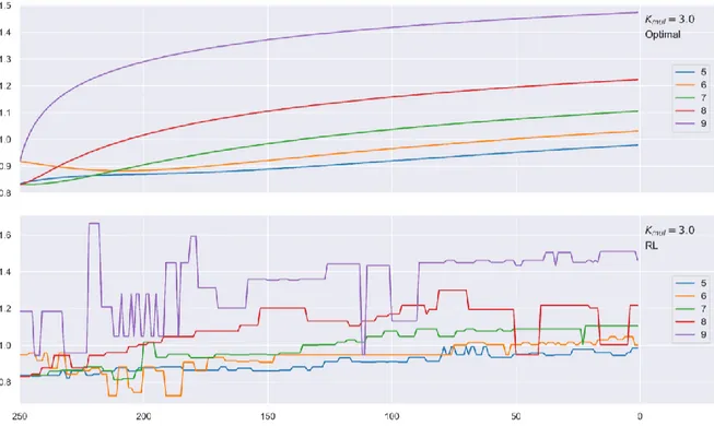
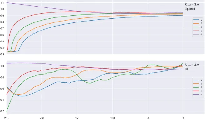
Appendix B – The reinforcement learning policy’s plot as a function of the time remaining until the backtesting process resumes ... 71
1 1 Introduction
In 1995, the Basel Committee on Banking Supervision issued an amendment to the first Basel Accord, Basel I. This amendment allowed financial institutions to develop internal risk models, based on the value-at-risk (VaR), as opposed to using the regulator’s predefined model. However, this liberty came at a cost, as the model’s ability to capture observed risk would be assessed on a yearly backtesting process, penalizing the market risk charge (MRC) as a function of the recorded violations. From this point onwards, the financial community focused its efforts on improving the accuracy of the VaR models to reduce the regulatory capital requirements. However, some authors proposed that the key towards disclosure optimization would not lie in improving the existing models, but in manipulating the estimated value. The most recent progress in this field employed dynamic programming (DP) based on Markov decision processes (MDPs), to create a daily report policy, based on the applicable regulation and the model’s ability to capture observed risk. An issue with the use of dynamic programming is the heavy cost involved. Firstly, the algorithm requires an explicit transition probability matrix, unfeasible in financial markets. This, paired with high computational storage requirements and an inability to operate in continuous MDPs, meant an alternative solution was needed.
In recent years, neural networks (NNs) have seen a widespread growth, boosting the fields which rely on its use, from computer vision to data science. However, the usage of these techniques within the financial sector has been long overdue, partly, due to the concerns over the lack of transparency of black-box methodologies. The purpose of this work is to introduce deep reinforcement learning (DRL) as an alternative to solving problems characterized by MDPs, whose dynamics have proven to be too complex or hard to map, usually the case in financial markets. The introduced class of algorithms do not require an explicit transition matrix, and therefore require little information about the underlying environment’s dynamics. Furthermore, some versions have the ability to learn continuous action and state spaces. In short, the goal of reinforcement learning is to provide an optimal policy which maps states to actions through a repeated trial-and-error process.
In order for the algorithm to be deemed viable to tackle this category of financial problems, its ability to converge towards a known optimal solution must be assessed, in other words, benchmarked, under the premise that should the algorithm prove capable of approximating a
2 simple problem’s solution, then surely its capability will be maintained when solving a complex environment, in which dynamic programming is not viable. For this purpose, proximal policy optimization (PPO), one of the most recent developments in DRL with improved convergence and stability in the continuous domain in comparison to its predecessors, has been selected to approximate the optimal solution computed by DP. In practice, the usage of algorithms with solid performance in discrete spaces, such as double dueling deep Q-network (DDQN), would be more appropriate for the selected benchmark as they can estimate the optimal solution faster and more efficiently – the algorithms in the policy gradient taxonomy, to which PPO belongs, tend to be stuck in local optima.
The problem selected for benchmarking is that of optimizing the value at risk disclosure under the second Basel Accord, characterized by discrete action and state spaces. The reasoning behind this selection is due to the fact that the problem in question has a complex and demanding environment, regarding its space dimensions, which could benefit from proximal policy optimization’s ability of learning under continuous spaces. This would therefore avoid many of the pitfalls and simplifications incurred to make the problem tractable for dynamic programming. The solution consists in the creation of a policy, that is, a map from actions to spaces, in which the state corresponds to a tuple of (a) the time remaining until the backtesting process is resumed, in days, in which the multiplier is reviewed as a function of the incurred exceedances, (b) in exceedances recorded to date, and lastly, (c) the applicable multiplier, for the relevant period. The policy is constructed via a proximal policy optimization agent, which learns the dichotomy between reporting low VaR values, minimizing the short-run cost, and the occurrence of exceedances, in which the observed loss surpasses the reported expected loss, leading to the next year’s multiplier to be modified.
The first part of this thesis introduces the applicable theoretical base, from the regulatory context which originates the need to optimize an internal model’s VaR disclosure, to the deep reinforcement learning theory, seeking to establish a link between dynamic programming and reinforcement learning. The focus then shifts to approximating the optimal policy generated by Seixas (2016), in addition to benchmarking the yielded solution with that of the mentioned author’s. Despite the small number of training iterations used in approximating the solution, the algorithm’s policy presented strong signs of convergence with the DP’s optimal policy, yielding similar results in behavior and incremental return, generated through the investment of the freed capital, whilst maintaining the institution’s exposure constant.
3 The thesis’ contribution to the field is therefore threefold: (a) it demonstrates the adequacy of deep learning in providing a solution to the Basel disclosure problem; (b) it paves the way for future improvements on the problem at hands via deep reinforcement learning; and lastly, (c) it introduces the class of deep reinforcement learning as a solution for optimization problems, a methodology long overlooked in the financial community.
4 2 Theoretical Framework
2.1 Basel Accords
In late 1974, in the wake of severe disturbances in the currency and banking markets, the G10 central bank governors established the Committee on Banking Regulations and Supervisory Practices. This committee was posteriorly renamed to Banking Committee on Banking Supervision (BCBS).
The BCBS was created as a regulatory body, providing a framework for global supervision and risk regulation. Nevertheless, the BCBS does not have legal power, nor has it pursued such goal. The institution’s purpose is, in short, to provide guidelines and standards on banking regulation, and to create a channel for cooperation and discussion between financial institutions. In July 1988, the Basel Committee on Banking Supervision presented a framework for measuring the capital adequacy, specifically, to establish the minimum levels of capital required for international banks. This documentation became known as Basel I, suggesting there would be further improvements to the document. The first Basel Accord focused mainly in credit risk, coupling the required capital level with the degree of credit risk in the institution’s portfolio. The latter’s assets would then be categorized into three buckets according to its risk, as perceived by the regulator. The regulation stipulated that financial institutions (FI) were required to hold a minimum of eight percent of capital in relation to risk-weighted assets – the capital adequacy ratio (CAR). Formally, this notion is expressed by the following formula:
𝐶𝐴𝑅 = 𝑇𝑖𝑒𝑟 𝐼 𝐶𝑎𝑝𝑖𝑡𝑎𝑙 + 𝑇𝑖𝑒𝑟 𝐼𝐼 𝐶𝑎𝑝𝑖𝑡𝑎𝑙
𝑅𝑖𝑠𝑘 𝑤𝑒𝑖𝑔ℎ𝑒𝑑 𝑎𝑠𝑠𝑒𝑡𝑠 𝑓𝑜𝑟 𝑐𝑟𝑒𝑑𝑖𝑡 𝑟𝑖𝑠𝑘100 , (1) where 𝑇𝑖𝑒𝑟 𝐼 𝐶𝑎𝑝𝑖𝑡𝑎𝑙, often referred to as core capital, comprises (a) paid up capital, (b) reserves and surplus, and (c) capital reserves and 𝑇𝑖𝑒𝑟 𝐼𝐼 𝐶𝑎𝑝𝑖𝑡𝑎𝑙, termed supplementary capital, refers to (a) undisclosed reserves, (b) revaluation reserves, (c) general provision and loss reserves, (d) hybrid (debt/equity) capital instruments, and € subordinated debt instruments. Additionally, the accord provided means of separating an institution’s assets into five different percentage categories, based on its risk nature, and accordingly, establishing each asset’s weight-factor.
5 Following general criticism that the standard approach defined in Basel I was incapable of accurately measuring risk, the BCBS incorporated market risk in capital requirements, reflecting the increasing tendency for FIs to increase their exposure to derivatives. In addition, the document introduced the ability for firms to self-regulate, as a means of encouraging risk taking and adequate measurement. The 1995 amendment to the first Basel Accord provided a framework for firms to assess the quality of their risk models through a backtesting process, as this methodology started to diffuse among FIs. Following this document, institutions were allowed to develop their own financial models to compute their market risk capital thresholds – the daily VaR. This archetype would be known as the Internal Model Approach (henceforth referred to as IMA). The backtesting process tied the market risk capital requirement, MRC, to both the portfolio’s risk, and the internal model’s quality. The market risk charge in a given day 𝑡, would then correspond to the combination of two components, the general risk charge and the specific risk charge
𝑀𝑅𝐶 = 𝐺𝑅𝐶 + 𝑆𝑅𝐶 , (2)
where GRC and SRC correspond to the general and specific risk charges, respectively. Whereas the GRC depended directly on the model, SRC represented the specific risk charge, a buffer against idiosyncratic factors, including basis and event risks. The former corresponded to the maximum between the present day’s value-at-risk, and the average of the last sixty daily risk disclosures, multiplied by a factor, which became known as 𝑘 or the multiplier factor. The condition stated in the previous sentence reflects in the following mathematical expression
𝐺𝑅𝐶𝑡 = max (𝑉𝑎𝑅𝑡,1%, 𝑘 ∗ 1 60∑ 𝑉𝑎𝑅𝑡−𝑖,1% 59 𝑖=0 ) , (3)
where the multiplier’s value, 𝑘, depended on the amount of violations verified during the backtesting process, and 𝑉𝑎𝑅𝑡,1% represents the 10-day value-at-risk computed at the 1% level.
6 Zone Number of Exceptions Potential Increase in K Multiplier Value (K) Cumulative Probability (%)1 Green 0 to 4 0.00 3.00 [8.11;89.22] Yellow 5 0.40 3.40 95.88 6 0.50 3.50 98.63 7 0.65 3.65 99.60 8 0.75 3.75 99.89 9 0.85 3.85 99.97 Red ≥10 1.00 4.00 99.97
Table 1 – The Basel Penalty Zones
The backtesting process would take place every 250 trading days, analyzing the entire period’s model estimates, with the VaR in question being computed at the 1% significance level. Table 1 summarizes the multiplier factor 𝑘’s states in relation to the recorded exceedances in the backtesting process for a given period.
In 2004, the BCBS released Basel II, the second Basel Accord. The document sought to further improve the risk management and capital adequacy guidelines set by Basel I, sixteen years earlier. The motivation behind this improvement lied in Basel I’s innability to differentiate risk, especially among members of the Organization for Economic Cooperation and Development (OECD), and the discrepancy between Basel I’s risk weights, and the actual economic risks. Whilst the first accord focused on credit risk, the new proposal integrated market (included in the 1996 ammendment) and operational risks on the minimum capital requirement computation. Another important addition in Basel II was the fact that assets’ credit rating played a major role in determining risk weights. Such reflected in riskier assets having larger weights, thus leading to a larger MRC.
Basel II created a three pillar structure, (a) minimum capital requirements, (b) supervisory review process and lastly, (c) market discipline. Regarding the first pillar (a), its goal was to provide a framework for calculating the required capital level for specific risk types, namely credit, operational and market risks. The first branch provided FIs with several alternatives for computing each of the risk types, thus enabling firms to choose that which suits their risk
1 “The probability of obtaining a given number or fewer exceptions in a sample of 250 observations when the
7 profile, enabing exceptional loss or economic crysis endurance. Pillar number two (b) provided details regarding how supervision should be organized in order to ensure the implementation quality of internal processes and controls, resulting in additional capital levels when applicable. Said pillar relied on the use of banking stress tests to assess an institution’s strength in adverse economic scenarios. Lastly, the third pillar (c) concerns transparency, referring to mandatory disclosures within each FI to the general public, thus enabling symmetric market information, whilst facilitating FI comparison.
At the time of the present work, the fourth Basel Accord was already showing signs of replacing its predecessor. However, since the content reflected throughout the document focuses on the second Basel Accord, the succeeding framework has not been further discussed.
2.2 Value at Risk
The value-at-risk is a statistical measure of potential loss, currently the market’s standard measure in assessing market risk. This concept can be defined as the maximum potential change in a financial portfolio’s value, with a certain probability, over an established period of time (Alexander, 2008).
According to Artzner et al. (1999), a risk measure 𝜌(∙) is to be considered coherent should it abide by four principles: (a) the monotonicity condition, which states that if a portfolio has lower returns than another portfolio for every state of the world, the latter’s risk measure should be greater than the former’s; (b) the translation invariance property, which establishes that if an amount of cash is added to a portfolio, its risk measure should go down by the same amount; (c) the homogeneity requirement in turn, stated that changing the size of a portfolio by a factor λ, while keeping the relative amounts of different items in the portfolio the same, should result in the risk measure being multiplied by λ; and lastly, (d) the subadditivity axiom states that the risk measure for two portfolios after they have been merged, should be no greater than the sum of their risk measures before said transformation. These conditions are represented mathematically in table 2.
8 Condition Name Condition Expression
Monotonicity 𝜌(𝑌) ≥ 𝜌(𝑋) 𝑖𝑓 𝑋 ≤ 𝑌
Homogeneity 𝜌(𝛼𝑋) = 𝛼𝜌(𝑋), ∀ 𝛼 > 0
Risk Free Condition 𝜌(𝑋 + 𝑘) = 𝜌(𝑋) − 𝑘, ∀ 𝑘
Subadditivity 𝜌(𝑋 + 𝑌) ≤ 𝜌(𝑋) + 𝜌(𝑌)
Table 2 – The four coherent risk measure conditions
Value-at-risk satisfies the first three conditions, but is not guaranteed to satisfy the fourth condition, the subadditivity axiom.
The value at risk can be described as the maximum loss which can be expected to occur if a portfolio is held static for a given amount of time ℎ, under a certain confidence level (1 − 𝛼) (Alexander, 2008). In a more practical view, it can be thought of as the amount of capital that must be added to a position to make its risk acceptable to regulators. This risk measure was introduced as an alternative to standard portfolio risk metrics, namely volatility and correlation, as these can only accurately measure risk when the asset’s or risk factor’s returns have a multivariate normal distribution. Value-at-risk encompasses a wide set of attractive features, namely the fact that it can easily be aggregated and disaggregated whilst taking into consideration the dependencies between its constituents; and its ability to not only measure the risk factor’s risk, but their sensitivities as well (Alexander, 2008).
Considering a significance level, 𝛼, such that, 0 < 𝛼 < 1, its quantile for a given distribution is given by
𝑃(𝑋 < 𝑥𝛼) = 𝛼 , (4)
Thus, the quantile 𝛼 of distribution 𝑋, 𝑥𝛼, can be obtained according to
𝑥𝛼= 𝐹−1(𝛼) , (5)
where 𝐹−1 represents the inverse of the distribution function.
Recall the VaR corresponds to the maximum loss which is expected to be exceeded with probability 𝛼, when the portfolio is held static for ℎ days. Accordingly, it corresponds to the computation of the 𝛼 quantile of the discounted ℎ-day P&L distribution:
9
𝑃(𝑋ℎ < 𝑥ℎ𝑡,𝛼) = 𝛼 , (6)
where 𝛼 corresponds to the significance level and 𝑋ℎ = 𝐵ℎ𝑡𝑃𝑡+ℎ−𝑃𝑡
𝑃𝑡 represents the ℎ-day
discounted return.
According to the previous statement, and since the value-at-risk is an estimated loss, its value can be obtained by direct application of equation (5):
𝑉𝑎𝑅ℎ,𝛼 = −𝐹𝐿−1(𝛼) , (7)
where 𝐹𝐿−1(𝛼) represents the inverse cumulative distribution function of losses.
By replacing the previous equation into (6) yields
𝑉𝑎𝑅ℎ,𝛼 = −𝑥ℎ𝑡,𝛼 , (8)
According to Simons (2000), the parametric linear framework is the most used of the three existing estimation methods, hence, this thesis’ focus. Within parametric methods, most research focuses on the use of normal distribution given its simplicity and the ability to use the ℎ-day square root, √ℎ, as a scaling rule for linear portfolios. It is important to note however, that this rule leads to a systematic underestimation of risk, where the degree of underestimation is aggravated the longer the time horizon, jump intensity2 and confidence level, failing to
address the objective of the Basel Accords (Danielsson & Zigrand, 2003). Nevertheless, this thesis will focus on the normal parametric value-at-risk and its scaling rule, given its well-known behavior and widespread use.
Assuming the portfolio’s discounted returns, 𝑋ℎ,𝑡 are i.d.d. and normally distributed with mean µ and standard deviation 𝜎, i.e.
𝑋𝑡,ℎ~ 𝑖𝑑𝑑
𝑁(𝜇ℎ𝑡, 𝜎ℎ𝑡2 ) , (9)
applying the normal standard transformation to the previous variable yields
𝑃(𝑋ℎ𝑡< 𝑥ℎ𝑡,𝛼) = 𝑃 (𝑍 <𝑥ℎ𝑡,𝛼− 𝜇ℎ𝑡
𝜎ℎ𝑡 ) = 𝛼 , (10)
where 𝑍 is a standard normal variable.
2 In The term jump refers to jump diffusion stochastic processes, models which aim at assessing the probability
of two i.d.d. variables modeled under the same distribution, seeing their price move significantly and synchronously.
10 Applying equation (5) to the previous expression results in the portfolio’s standardized discounted return’s inverse cumulative function
𝑥ℎ𝑡,𝛼− 𝜇ℎ𝑡
𝜎ℎ𝑡 = Φ
−1(𝛼) , (11)
Because the normal distribution is symmetric around its mean, then the previous expression can be rewritten as
𝜙−1(𝛼) = −𝜙−1(1 − 𝛼) , (12)
Plugging the previous expression into (7) yields the formula of the value-at-risk with drift adjustment
𝑉𝑎𝑅ℎ𝑡,𝛼 = 𝜙−1(1 − 𝛼)𝜎ℎ𝑡− 𝜇ℎ𝑡 , (13)
where 𝜇ℎ𝑡 represents the drift adjustment.
Under the assumption that the portfolio’s expected return is the risk-free rate, 𝜇ℎ𝑡= 0, and dropping the implicit dependence of VaR on time 𝑡, the previous expression can be further simplified as
𝑉𝑎𝑅ℎ,𝛼 = 𝜙−1(1 − 𝛼)𝜎ℎ , (14)
Under the assumption that the returns follow a normal distribution, the h-day VaR can be obtained resorting to the square root scaling rule, that is
11 2.3 Markov Decision Process
Markov decision processes, or simply, MDP’s, are comprised of a set of spaces 𝒮, a vector of possible actions 𝒜, a transition and reward models. Miranda & Fackler (2002) sum up a MDP by a choice to be taken at each time step t, 𝑎𝑡, from the available relevant action set for the present state 𝑠𝑡, 𝒜(𝑠𝑡), earning a reward 𝑅𝑡 , from a function parametrized by both current state and selected action.
Figure 1 – The figure shows the agent-environment interaction in a Markov decision process, where the agent interacts with the environment by performing the selected action, and the environment returns the reward and new state associated with the
agent’s behavior.
The transition model defines which state the environment transitions to, contingent on the present state and selected action,
𝒫𝑠𝑠′𝑎 = 𝑃(𝑠′|𝑠, 𝑎) = ℙ[𝑆𝑡+1= 𝑠′|𝑆𝑡= 𝑠, 𝐴𝑡 = 𝑎] , (16)
where ℙ denotes a probability function.
The reward function on the other hand, defines the reward yielded at time step 𝑡, contingent on the current state 𝑠 and selected action 𝑎
𝑅𝑡 = 𝑅(𝑠𝑡, 𝑎𝑡) , (17)
These two components, the transition and rewards models, form the basis of a Markov decision process.
Markov introduced the concept of memorylessness of a stochastic process, a key propriety of MDPs. This assumption states that each state pair is independent of past-occurrences, meaning, each state contains all the meaningful information from the history. In other words, the future
12 and past are conditionally independent given the present, since the current state contains all the required statistical information to decide upon the future.
The concept of policy, represented by the symbol π, which corresponds to a mapping from states to actions, is meaningful throughout the course of this work. Policies can be deterministic or stochastic. The former corresponds to a policy in which the optimal action is solely determined by the current state. The probability of an action being selected in state 𝑠 under a deterministic policy 𝜋 is given by
𝜋(𝑠) = 𝑎 , (18)
whereas if the policy 𝜋 is stochastic, the action selection is contingent on a probability function
𝜋(𝑎|𝑠) = ℙ[𝐴𝑡= 𝑎|𝑆𝑡 = 𝑠] , (19)
Value functions, 𝑣𝜋(𝑠) attribute a quantifiable goodness value to a given state under a policy 𝜋, by attempting to capture its associated future reward. The latter corresponds to the sum of discounted future rewards, or expected return, given by 𝐺𝑡
𝐺𝑡= ∑ 𝛾𝑘−𝑡−1𝑅 𝑘 𝑇
𝑘=𝑡+1
, (20)
where 𝛾 ∈ [0,1] represents the discount term, a factor by which to penalize future rewards. The state-value function of a given state 𝑠 at time 𝑡, corresponds to the expected reward the algorithm is to observe starting from state 𝑠
𝑣𝜋(𝑠) = 𝔼𝜋[𝐺𝑡|𝑆𝑡= 𝑠]
= 𝔼[𝑅𝑡+1+ 𝛾𝑣(𝑆𝑡+1)|𝑆𝑡= 𝑠] , (21)
where 𝔼𝜋[∙] represents the expected value of a given random variable considering the agent
follows policy 𝜋.
Whilst the value function focuses on individual states, the action-value function 𝑞𝜋, seeks attributing a fitness value for the action as well,
𝑞𝜋(𝑠, 𝑎) = 𝔼𝜋[𝐺𝑡|𝑆𝑡 = 𝑠, 𝐴𝑡 = 𝑎]
= 𝔼[𝑅𝑡+1+ 𝛾𝑞𝜋(𝑆𝑡+1, 𝐴𝑡+1)|𝑆𝑡 = 𝑠, 𝐴𝑡 = 𝑎] ,
13 Using the probability distribution over all possible actions and q-values, that is, state-action values, the value function can be obtained by
v𝜋(𝑠) = ∑ 𝑞𝜋(𝑠, 𝑎)𝜋(𝑎|𝑠) 𝑎∈𝒜
, (23)
The overall objective under the MDP framework is to compute the value function which maximizes the rewards, 𝑣𝜋∗(𝑠) ≥ 𝑣𝜋(𝑠) ∀ 𝜋, 𝑠 ,
𝑣∗(𝑠) = max
𝜋 𝑣𝜋(𝑠) (24)
𝑞∗(𝑠, 𝑎) = max
𝜋 𝑞𝜋(𝑠, 𝑎) , (25)
The previous goals can be achieved via Bellman’s optimality equations v∗(𝑠) = max 𝑎 𝔼[𝑅𝑡+1+ 𝛾𝑣∗(𝑆𝑡+1)|𝑆𝑡 = 𝑠, 𝐴𝑡 = 𝑎] (26) 𝑞∗(𝑠, 𝑎) = 𝔼[𝑅𝑡+1+ 𝛾 max 𝑎′ 𝑞∗(𝑆𝑡+1, 𝑎 ′)|𝑆 𝑡 = 𝑠, 𝐴𝑡= 𝑎] , (27)
The reinforcement learning models and concepts presented and used throughout this thesis, assume problems described by infinite horizon, stochastic transition model MDPs.
2.4 Proximal Policy Optimization
The current section presents, in a concise manner, the main ideas behind the proximal policy optimization algorithm, on which the agent applied in this thesis is based. For those unfamiliar with the topic, Appendix A attempts to shed light on the deep reinforcement learning algorithm taxonomy, starting with familiar concepts such as dynamic programming and Monte Carlo returns, to the present section’s algorithm’s predecessor, trust region policy optimization (TRPO). Note however, that the appendix merely scratches the surface in terms of reinforcement learning’s literature. It is important to mention that there are several important and widely used algorithms not present in the referred section, which form the cornerstone of deep reinforcement learning. For instance, asynchronous advantage actor-critic (A3C) and its synchronous and deterministic version (A2C), deterministic policy gradient (DPG), deep deterministic policy gradient (DDPG), both of which, model the policy as a deterministic
14 decision, distributed distributional DDPG (D4PG), actor-critic with experience replay (ACER), actor-critic using Kronecker-Factored trust region (ACKTR), soft actor-critic (SAC). However, in order to keep the algorithmic literature review as concise as possible, these have been left out of the present discussion. These algorithms form a clear timeline of deep reinforcement learning’s evolution, thus, understanding them, may help clarifying and solidifying the employed concepts.
The trust region policy optimization algorithm introduced in Appendix A.III – Policy Gradient has a few shortcomings, namely, the computation of the Fisher matrix at every model parameter update, which is computationally expensive, and its requirement of large batches of rollouts to approximate the the Fisher matrix accurately.
Proximal policy optimization (Schulman, et al., 2017) is an on-policy algorithm, able to learn control problems under discrete or continuous action spaces, which seeks providing the answer for the same question as its predecessor, TRPO, does: to what extent can the policy be updated, using the available information, without modifying it too largely, which would result in performance collapse. Whereas TRPO provides the answer relying on the use of a complex second-order method, PPO is comprised of a set of first-order equations, combined with a few tricks, which ensure the similarity between the old and new policies.
Consider the probability ratio between the old and new policies
𝑟(𝜃) = 𝜋(𝑎|𝑠, 𝜃)
𝜋(𝑎|𝑠, 𝜃𝑜𝑙𝑑) , (28)
Under the previous construct, TRPO’s objective function can be represented as
𝐽𝑇𝑅𝑃𝑂(𝜃) = 𝐸 [𝑟(𝜃)𝐴̂
𝜋𝜃𝑜𝑙𝑑(𝑠, 𝑎)] , (29)
The previous equation represents another of TRPO’s shortcomings not mentioned in the previous paragraph. Should the distance between policies not be bounded, then the algorithm would suffer from instability, caused by large parameter updates and large policy ratios. PPO imposes a constraint on this ratio, by ensuring 𝑟(𝜃) stays within the range [1 − 𝜖, 1 + 𝜖], where 𝜖 is the clipping hyperparameter.
15 The new objective function, a surrogate function, is referred to as the Clipped3 objective function, and is represented by 𝐽𝐶𝐿𝐼𝑃(𝜃)
𝐽𝐶𝐿𝐼𝑃(𝜃) = 𝐸 [(𝑟(𝜃)𝐴̂𝜋
𝜃𝑜𝑙𝑑(𝑠, 𝑎), 𝑐𝑙𝑖𝑝(𝑟(𝜃), 1 − 𝜖, 1 + 𝜖)𝐴̂𝜋𝜃𝑜𝑙𝑑(𝑠, 𝑎)) ] , (30)
where 𝑐𝑙𝑖𝑝(∙) represents the clipping function, which ensures the first argument, is bounded by the remaining arguments.
The introduced objective function takes the minimum between the policy’s ratio, and the clipped arguments, therefore preventing excessively large (𝜃) updates, especially when associated with very large rewards – which would result in extreme policy updates.
The version of proximal policy optimization employed throughout this thesis, corresponds to the algorithm’s Clip or clipped version, under the actor-critic framework. In order to accommodate the actor-critic framework, the authors augmented the objective function with an error term on the value function, whilst adding an entropy term to encourage exploration.
𝐽𝐶𝐿𝐼𝑃′(𝜃) = 𝐸 [𝐽𝐶𝐿𝐼𝑃(𝜃) − 𝑐
1(𝑉𝜃(𝑠) − 𝑉𝑡𝑎𝑟𝑔𝑒𝑡) 2
+ 𝑐2𝐻(𝑠, 𝜋𝜃(𝑎|𝑠))] , (31)
where 𝑐1 corresponds to the error term coefficient, and 𝑐2 to the entropy coefficient, both of
which, are hyperparameters.
Algorithm Proximal Policy Optimization with Clipped Objective
1. Input: initial policy parameters 𝜃0, initial value function parameters 𝜙0
2. for 𝑘 = 0,1,2, … do
3. Collect a set of partial trajectories 𝒟𝑘 = {𝜏𝑖} by running policy 𝜋𝑘 = 𝜋𝜃𝑘 in the
environment
4. Compute rewards-to-go 𝑅̂𝑡
5. Compute advantages estimates, 𝐴̂𝜋𝜃𝑜𝑙𝑑𝑡, using any advantage estimation algorithm based on
the current value function 𝑉𝜙𝑘
6. Update the policy by maximizing the Clipped PPO objective: 𝜃𝑘+1 = argmax
𝜃 ℒ𝜃𝑘(𝜃)
by taking K steps of minibatch stochastic gradient ascent via Adam where ℒ𝜃𝑘 = 𝔼𝑡~𝜋𝑘[∑ [min (𝑟𝑡(𝜃)𝐴̂𝜋𝜃𝑜𝑙𝑑𝑡, 𝑐𝑙𝑖𝑝(𝑟𝑡( 𝜃), 1 − 𝜖, 1 + 𝜖))] 𝑇 𝑡=0 𝐴̂𝜋 𝜃𝑜𝑙𝑑𝑡 ] end for
Algorithm 1 – Proximal policy optimization pseudo-code.
3 The function is not named PPO’s objective function, as the algorithm introduces two versions of the objective
function, PPO-Penalty and PPO-Clip. However, the author opted for only introducing the latter as it corresponds to the version used in this thesis.
16 3 Literature Review
Since the early 1990’s, Value-at-Risk has increasingly become the standard for risk measuring and management throughout a wide range of industries. However, the concept attained special relevance with the 1995 amendment to the first Basel Accord, which enabled FI’s to develop and use their own internal models, as described in section 2.1. Ever since, the literature on value-at-risk, ranging from its estimation to its optimization under the Basel Accord framework, has grown uninterruptedly. The present chapter focuses on introducing past findings on the subject at hands and summarizing the corresponding author’s findings.
In 2007, Pérignon et al. (2007) introduced the notion that commercial banks tend to over-report their VaR estimate. The authors found three possible justifications for this fact. Firstly, incorrect risk aggregation methods induce higher VaR estimates by improperly accounting for the diversification effects. Secondly, banks tend to overstate their VaR metric to protect their reputation, as any evidence that the institutions are incapable of accurately measure their risk, would result in market-driven penalties. Lastly, a typical principal-agent problem takes place, where the risk manager voluntarily increases the VaR estimate to avoid attracting unwanted attention. Such behavior not only represents higher costs for the banks in terms of larger allocated capital and corresponding opportunity costs, but to the economy as well. Specifically, according to the author, the tendency to over-report risk leads to an exaggerate estimate of a bank’s implicit risk from an investor’s point of view, influencing its asset-pricing through the increase of required return on equity thus generating market distortions; furthermore, the excessive capital allocation leads to the rejection of funding for relevant projects, creating a loss of value for the economy.
With the introduction of the second Basel Accord, McAleer (2008) suggested a set of ten practices which aimed at helping FIs monitor and measure market risk, in order to minimize the daily capital charge, in particular when the FI focuses in holding and moving cash, rather than on risky financial investments. The author provided insights on (a) choosing between volatility models; (b) the underlying distribution’s kurtosis and leverage effects; (c) the covariance and correlation relationship models; (d) the use of univariate or multivariate models to forecast the value-at-risk; (e) the underlying distribution’s type selection according to the volatility type (conditional, stochastic or realized; (f) optimal parameter selection; (g) assumption derivation; (h) forecasting model’s accuracy determination; the penultimate point,
17 (j) optimizing the FI’s exceedances, which constitutes the object of this thesis; and lastly, (k) exceedance management and its relationship with the public interest.
In the aftermath of McAleer (2008)’s findings and recommendations on risk measurement and daily capital charge optimization, McAleer et al. (2009) introduced a model which attempted to design a rule to minimize the daily capital charges for institutions working under the Basel II regulation. This methodology, entitled the dynamic learning strategy (DYLES), was characterized by discrete and fast reactions whenever exceedances were recorded, being context sensitive in the sense that it accommodated past information, or violation history, onto its estimate, behaving more cautiously or conservatively when more exceedances had been recorded, and aggressively otherwise.
The authors formalized DYLES as:
min Θ=[𝑃0,𝜃𝑃,𝜃𝑅] 1 250∑ max [−𝑃𝑡𝑉𝑎𝑅(𝑡 − 1), [3 + 𝑘] 1 60∑ −𝑃𝑡𝑉𝑎𝑅(𝑡 − 𝑝) 60 𝑝=1 ] 250 𝑝=𝑗 , (32)
where 𝑃𝑡 is a variable which is tied to the number of recorded exceedances, representing how
aggressive or conservative the estimate is regarding the estimated risk measure, the value-at-risk; 𝜃𝑃 and 𝜃𝑅 are, respectively, the penalty per violation and the 25-day accumulated reward; p represents the backtesting time step, from 1 to 250; and k represents the applicable multiplier increment, applied to 3, from the value set [0.0; 0.4; 0.5; 0.65; 0.75; 0.85; 1], should there be more than 4 recorded exceedances in the previous financial year. Lastly, t represents, as usual, the date in which the system is being modeled in. The authors concluded that in all occasions, using the DYLES strategy led to higher capital savings when compared to a passive behavior, that is, disclosing the computed VaR, decreasing the capital requirements by 9.5%, on average, up to 14%, and reducing, on average, the number of violations from 12 to 8.
Kuo et al. (2013) proposed a modification to the DYLES decision rule, attempting to incorporate the challenges faced by banks created by the Basel III reforms as noted by Allen et al. (2012). In order to do so, Kuo et al. (2013) added the current market cost of capital to the DYLES rule, naming it, MOD-DYLES. The improved model not only allowed higher cost savings when compared with the original DYLES methodology, but it also enabled its extension to other VaR computation methods (Kuo, et al., 2013). The authors analyzed three strategies – standard unmanipulated disclosure, DYLES-based approach and the proposed MOD-DYLES model – for two VaR estimation methods, the constant covariance, and the variance-covariance GARCH methods. For the first estimation method, Kuo et al. (2013) observed that
18 MOD-DYLES introduced an average saving of 1.36% when compared to the passive standard disclosure approach, whilst drastically decreasing violations. Focusing on its predecessor, the modified algorithm managed to save, on average, an extra 0.10% per year, although as expected given their identical underlying exceedance constraints, the number of recorded violations matched. Regarding the second estimation model, the VC-GARCH, the proposed framework saved on average 1.09% and an extra 0.06% per year, respectfully, for the standard disclosure, in comparison with DYLES.
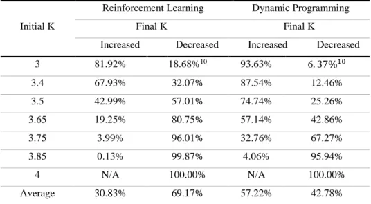
Seixas (2016) sought to further exploit the concept first introduced by McAleer (2008) that the path to optimization should not focus exclusively on the VaR estimation method, but also on the percentage of the metric which should be disclosed, as a form of capital charge minimization. The researcher’s work emphasized the need to construct an optimal policy for the daily VaR disclosure, under the internal model approach, as proposed by the Basel II Accords. In order to do so, Seixas (2016) applied the dynamic programming methodology to the problem at hands, using a discrete MDP with infinite periods. The author managed to create a policy which minimized the daily capital charge, considering (a) the time remaining until the back process takes place, (b) the number of recorded exceedances until the moment of decision, and lastly, (c) the applicable multiplier as defined by the preceding financial year’s backtesting process. The policy generated tended to underreport the one-day value-at-risk, that is, to adopt an aggressive approach, which is consistent with McAleer et al. (2009)’s notes on risk manager’s behavior. The use of the dynamic programming framework allowed surpassing some of the limitations and obstacles faced by DYLES’s, namely, its employment being contingent on the portfolio at hands, and the parameter estimation problem, which would represent a different disclosure rule contingent on the underlying distribution. When compared to the standard option of disclosure based on a normal distribution’s strategy, Seixas (2016)’s proposal outperformed the normal strategy in 82% of the times, yielding an average saving of 7.22% per day, when applied to a S&P500 portfolio.
19 4 Methodology
The purpose of the current chapter is twofold. Firstly, it models the Basel framework introduced in section 2.1 into a Markov decision process suitable for deep reinforcement learning. Secondly, the author covers the introduction and assessment of an agent, based on proximal policy optimization under the actor-critic framework, which attempts to approximate Seixas (2016)’s solution to the Basel problem.
4.1 Environment Model
The problem at hands has been thoroughly introduced in chapter 2.1. The current section turns to formalizing the environment so it can be solved via DRL.
Recall that the model, under the model-free reinforcement learning framework, is comprised of three components, the state and action spaces, and the reward function. The agent’s goal under the proposed environment, is to minimize the daily regulatory capital charge (𝑘 ∗ 𝑥 ∗ 𝑉𝑎𝑅𝑡) by optimizing the percentage of the value-at-risk to disclose, 𝑥. The problem represents a trade-off between opting to minimize the short-term disclosure – thus obtaining larger daily rewards – and the long-term cost, in the shape of the applicable multiplier, a direct function of the incurred exceedances, which in turn, are partly4 dictated by the value-at-risk manipulation. The state-space is characterized by three key aspects: (a) the time remaining until the backtesting process takes place (TtoB); (b) the number of recorded exceedances in the current trading period (EC); and lastly, (c) the applicable multiplier (K) throughout the given period. The first constituent, TtoB, corresponds to how much time, measured in days, remains until the new regulatory backtesting process starts, that is, before the year’s disclosure is accounted for, and its quality assessed, considering 250 trading days. The variable’s natural behavior is then to decade from its maximum value, until 1, when the review procedure takes place. The second flag, represented by the acronym EC, accounts for the number of exceedances recorded in the current episode. The set of possible values for this variable starts at 0, where no exceedance has been registered, and its maximum value is set at 11. The reasoning for the limitation to 11 exceedances is due to the fact that any further violations would still place the
4 The idea of partial responsibility in the action selection in determining the next period’s applicable multiplier
20 FI on the highest multiplier, hence, rational behavior dictates that at this point, the institution would report a null value-at-risk, so as to decrease the short-term costs. However, the environment is modeled under the assumption that reaching the 10-exceedance threshold, would translate in the FI not being able to deploy its internal model, being forced by the regulator to use a standard risk model instead. For this reason, the agent is incentivized to avoid the 10th exceedance at all costs, being forced to report the maximum disclosure value, under the assumption that reaching said threshold would imply the FI incurring in high reputational costs. The third variable’s values correspond to those defined in table 1. Accordingly, the state space corresponds to a 3-dimensional vector, comprised of the three discrete variables defined above, that is, one where each observation is a tuple comprised of one element of each discrete group. Specifically, 𝒯 = {𝜏 | 𝜏 ∈ ℤ, 1 ≤ 𝑥 ≤ 250}, ℰ = {𝜖 | 𝜖 ∈ ℤ, 0 ≤ 𝑥 ≤ 11} and 𝒦 = {3, 3.4 , 3.5 , 3.65 , 3.75, 3.85, 4, 10000}, which correspond to the time, exceedance and multiplier spaces, respectively. Accordingly, an observation under the current environment is defined as
𝑠𝑡 = (𝜏 ∈ 𝒯, 𝜖 ∈ ℰ, 𝜅 ∈ 𝒦) , (33)
Note, however, the inclusion of an additional multiplier in 𝒦, corresponding to 10000, which corresponds to a bankruptcy state, thus being represented by an extreme value, one which the institution would avoid at all cost.
In turn, the action space comprises the possible disclosure values, in percentage of the reported value, corresponding to values in the interval ]0, 3] with increments of 1𝐸−3, that is,
𝒜 = {𝑛/1000 | 𝑛 ∈ ℕ+, 𝑛 ≤ 3000} , (34)
where reporting the space 𝒜’s ceiling corresponds to a situation where VaR disclosure is threefold, and vice-versa.
Despite being a model-free algorithm, a simulator must be present to be able to generate new samples from which the agent can learn. Such simulator describes the transitioned state 𝑠𝑡+1, contingent on the current state 𝑠𝑡 and the selected action 𝑎𝑡, 𝒫𝑠𝑠′𝑎 . For the purpose of solving the described problem, a simple transition simulator based on Seixas (2016) has been used. Such entity is governed by the table which follows
21
Event Probability
No Exceedance 𝑃(𝑍 < 𝑉𝑎𝑅 ∗ 𝑥)
Exceedance 1 − 𝑃(𝑍 < 𝑉𝑎𝑅 ∗ 𝑥) − 𝑃(𝑍 > 𝐶𝑎𝑝𝑖𝑡𝑎𝑙 𝐶ℎ𝑎𝑟𝑔𝑒)
Bankruptcy 𝑃(𝑍 > 𝐶𝑎𝑝𝑖𝑡𝑎𝑙 𝐶ℎ𝑎𝑟𝑔𝑒)
Table 3 – Transition probabilities for the simulator
where 𝑍 is a standardized normal distribution of profit and loss, under which, the probabilities are yielded by
𝑃(𝑍 < 𝑉𝑎𝑅 ∗ 𝑥) = Φ(𝑥 ∗ 𝑉𝑎𝑅𝛼,ℎ, 𝜇, 𝜎) (35)
𝑃(𝑍 > 𝐶𝑎𝑝𝑖𝑡𝑎𝑙 𝐶ℎ𝑎𝑟𝑔𝑒) = 1 − Φ(𝑘𝑡∗ 𝑉𝑎𝑅𝛼,ℎ ∗ √10, 𝜇, 𝜎) , (36)
One of the critical aspects of reinforcement learning is the reward function. Such construction is target of a both feature engineering, and prior domain knowledge. A surrogate reward function is introduced to help the algorithm converge to the optimal policy faster and more accurately, given its episodic nature. Specifically, an additional reward is given when the backtesting process occurs. Mathematically, 𝑓(𝑎𝑡, 𝑠𝑡) is given by
𝑓(𝑎𝑡, 𝑠𝑡) = 𝑓(𝑎𝑡, [ 𝑡𝑡𝑜𝑏, 𝑒𝑐, 𝑘]𝑡) = −𝑘𝑡∗ 𝑎𝑡∗ 𝑉𝑎𝑅1,0.01∗ √10 + 𝐼𝑡(𝑠𝑡) ∗ ℛ(𝑠𝑡) , (37)
where 𝑉𝑎𝑅1,0.01 represents the one day value-at-risk computed at the 1% significance level, and
𝐼𝑡(𝑠𝑡) is an indicator function, which takes the value one if the episode’s time remaining to
backtesting (Ttob) equals one, and zero otherwise,
𝐼𝑡(𝑠𝑡) = { 1 0 𝑖𝑓 𝑖𝑓 𝑇𝑡𝑜𝐵𝑡= 1 𝑇𝑡𝑜𝐵𝑡 = 0 , (38)
and ℛ(𝑠𝑡) corresponds to the terminal reward space,
ℛ(𝑠𝑡) = −10𝐸3 ∗ {
𝑅(𝑘 = 0) + (𝐾𝑖− 𝐾𝑖+1)/2 , 1 ≤ 𝑘 ≤ 6
0.1, 𝑘 = 0
0, 𝑘 = 7
, (39)
Applying the previous equation, yields the eight additional reward factors
ℛ(𝑠𝑡) = [0.1, 0.3, 0.35, 0.425, 0.475, 0.525, 0.6, 0] ∗ (−10𝐸3) , (40)
The introduced surrogate reward aims at accelerating learning by injecting domain knowledge directly into the reward space, filling in the gap left by the use of episodic reinforcement
22 learning (RL). By doing so, the long-term objective is hardcoded into the agent which would otherwise be unperceived, as under episodic RL the agent never reaches the next period where the multiplier revision is materialized. The additional reward space attempts to capture the multiplier distribution’s underlying structure, by measuring the difference between multipliers, and scaling the gradient to the reward distribution’s parameters, a behavior similar to that of McAleer et al. (2009). Notice that the last multiplier, associated with bankruptcy, has a null reward, which is counterintuitive, as rationale dictates such state should be associated with additional penalties – the additional rewards are negative, according to the standard reward distribution. The reasoning behind such formulation, is that the reward for defaults is extremely negative, hence, penalizing the behavior further will only hinder policy gradients by contributing to the occurrence of exploding gradients, whilst producing no additional information. However, the additional space introduces a bias towards exceedances up to 4 (with the lowest multiplier), as the agent may seek exploiting this lower penalty - or higher reward. Yet, due to the small number of iterations, the author saw fit adding it to accelerate learning. For researchers aiming to solve the problem with more iterations, it is not advisable to use the proposed modification without extensive testing.
Note that during training, the reward function has been scaled to the [-1, 0] range, to prevent exploding gradients and to ease gradient descent’s functioning, as is typical in DRL literature. The algorithm’s network is the same for both actor and critic, 2 hidden layers, each containing 64 neurons, the first layer using a Rectified Linear Unit (ReLu) (Agarap, 2019) activation function for both entities. Activation functions are needed to create non-linear transformations, as a neural network is only capable of performing linear transformations without non-linear activation functions. To understand more deep learning concepts such as neural networks and their architectures, the reader is advised to delve into Goodfellow et al. (2016).
Deep learning algorithms can prove troublesome to understand and implement, particularly for those delving in the class of algorithms for the first time. For this reason, and to remove some of the conceptual abstraction, the remainder of the present section attempts to represent in simple terms the operations performed in a simple version of PPO, that is, to create an implementation pseudo-code. In practice, typical implementations rely on the use of Generalized Advantage Estimators (GAE), multithreading, among other useful modifications to simplify and speed computations and help convergence. These have been omitted from the
23 representation. Yet, to demonstrate the easiness of the algorithms in accommodating a variety of situations, the scheme presents the process for both discrete and continuous actions.
Algorithm Actor Critic PPO Implementation
1. Define the learning constants
1.1 E_MAX : Maximum number of episodes 1.2 E_LEN : The episode’s length
1.3 𝛾 : The discount factor 𝛾 1.4 𝛼𝐴 : Actor’s Learning Rate
1.5 𝛼𝐶: Critic’s Learning Rate
1.6 MIN_BATCH_SIZE : Minimum batch size for updates
1.7 A_UPDATE_STEPS: Actor’s update operation n-step loop length 1.8 C_UPDATE_STEPS: Critic’s update operation n-step loop length 1.9 𝜖: Surrogate objective function clip term 𝜖
1.10 S_DIM : State space shape 1.11 A_DIM : Action space shape 2. Initialize the critic:
2.1 Input layer: Dense layer input: S_DIM shape: [64, 1] activation: ReLu trainable: True 2.2 Hidden Layer: Dense Layer
input: Input layer (2.1) shape: [64, 1]
activation: ReLu trainable: True
2.3 Value Estimation Layer - Output Layer: Dense layer input: Hidden Layer (2.2)
shape: 1
activation: None trainable: True
3. Define the critic’s Optimization Function: 3.1 𝐴̂θ(𝑠, 𝑎) = 𝑟 − 𝑉(𝑠)
3.2 Define the loss function: 𝐴̂θ(𝑠, 𝑎)2
3.3 Optimization function c_trainop: Adam Optimizer: learning rate: 𝛼𝐶
minimization target: 3.2
4. Define the actor (𝜋): 4.1 Input layer: Dense layer
input: S_DIM shape = [64, 1] activation = Relu trainable = True 4.2 Hidden Layer: Dense layer
input: Input layer (4.1) shape: [64, 1]
activation: ReLu trainable: True
24 4.3 Action (𝜋) Layer - Output Layer : Dense Layer
input: Hidden Layer (4.2) shape: A_DIM
activation: Softmax trainable: True
5. Define the old actor (𝜋𝑜𝑙𝑑):
5.1 𝜋𝑜𝑙𝑑= 𝜋, only the former is not trainable
6. Define the Actor’s Optimization Function 6.1 Compute the probability ratio 𝑟(𝜃) = 𝜋(𝑎|𝑠,𝜃)
𝜋(𝑎|𝑠,𝜃𝑜𝑙𝑑)
6.2 Compute the Surrogate Loss 𝑟(𝜃) ∗ 𝐴̂θ(𝑠, 𝑎)
6.3 Compute PPO’s Clipped Loss = − min (𝑟
𝑡(𝜃)𝐴̂𝑡
𝜋𝑘, 𝑐𝑙𝑖𝑝(𝑟
𝑡( 𝜃), 1 − 𝜖, 1 + 𝜖))
6.4 Optimization Function a_trainop:
Adam Optimizer: learning rate: 𝛼𝐴,
minimization target: (6.3)
7. Define the Update Function
7.1 Receive input: state 𝑠, action 𝑎, reward 𝑅 7.2 Replace 𝜋𝑜𝑙𝑑 with 𝜋
7.3 Compute 𝑉(𝑠) using the Critic (2.) 7.4 Compute the advantage function (3.1)
7.5 Update the Actor using PPO’s clipping method: execute a_trainop for A_UPDATE_STEPS 7.6 Update the Critic: execute c_trainop for C_UPDATE_STEPS
8. Run the Simulation
8.1 Build the environment env 8.2 for ep in E_MAX
8.2.1 Reset the environment and observe 𝑆
8.2.2 Define the state, action and reward buffers 𝒟𝑠, 𝒟𝑎, 𝒟𝑟
8.2.3 for 𝑡 in E_LEN:
8.2.3.1 𝑎 = 𝜋(𝑠)
8.2.3.2 Perform 𝑎 and observe S’ and 𝑅
8.2.3.3 Add state, action and reward to the corresponding buffers 𝒟𝑠+= 𝑠
𝒟𝑎+= 𝑎
𝒟𝑟+= 𝑅
8.2.3.4 Set 𝑆′ = 𝑆
8.2.5.5 If 𝑙𝑒𝑛𝑔𝑡ℎ(𝑆) ≥ 𝑀𝐼𝑁_𝐵𝐴𝑇𝐶𝐻_𝑆𝐼𝑍𝐸: 8.2.5.5.1 Compute 𝑉(𝑆) using the Critic (2.)
8.2.5.5.2 Compute the 𝑉(𝑠𝑡) for each reward in the buffer, inserting it into a buffer
𝑉𝑡= 𝑟𝑡+ 𝛾𝑉𝑡+1
𝐷𝑟𝑑𝑖𝑠𝑐+= 𝑉𝑡
8.2.5.5.3 Update PPO (7.) using 𝒟𝑠, 𝒟𝑎, 𝒟𝑟𝑑𝑖𝑠𝑐
8.2.5.5.4 Set 𝒟𝑠= 𝒟𝑎= 𝒟𝑟 = 𝒟𝑟𝑑𝑖𝑠𝑐 = 𝐸𝑚𝑝𝑡𝑦
8.2.4 end for
8.3 end for
25 Throughout this thesis numerous advantages of using DRL versus DP have been appointed, with section 4.2.6 providing a more exhaustive list of the advantages of using the current class of algorithms. One of which, is the ease to adapt and modify the model’s architecture. The previous pseudo-code illustrates how both the actor and critic’s structure can be changed by simply plugging additional hidden layers, which can be done programmatically. Another mentioned key aspect is the ability to include continuous state and actions spaces. In fact, the inclusion of a continuous action space estimation merely involves a small change to the critic’s architecture, requiring the underlying distribution’s parameters – in the following case, a univariate Gaussian’s mean and standard deviation - to be optimized, instead of the critic’s network 𝜋. Specifically, the point 4. In the previous pseudo-code would be modified to the following
Algorithm Actor Critic PPO Implementation – Actor under a Gaussian probability distribution
4. Define the actor (𝜋): 4.1 Input layer: Dense layer
input: S_DIM shape [64, 1] activation: ReLu trainable: True 4.2 𝜇 Layer: Dense layer
input: Input layer (4.1) shape: A_DIM
activation: Tahn trainable: True 4.3 𝜎 Layer: Dense layer
input: Input layer (4.1) shape: A_DIM
activation: Softplus trainable: True 4.4 return 𝑁~(𝜇, 𝜎)
Algorithm 3 – A modification to Algorithm 2 to encompass continuous actions.
4.2 Results
The purpose of the current work is not to yield a policy better than that of Seixas (2016)’s, given it represents an optimal policy, nor to fully reproduce the author’s result, but is instead, to demonstrate the capabilities of deep reinforcement learning in approximating a solution to the same problem, whilst bypassing some dynamic programming’s hindrances. Hence, the section will be divided into three parts. The first section will focus on the computational requirements used in training the model, whilst providing a few insights into the process of
26 estimating an increasingly optimal policy under the DRL framework. The second section shifts the attention towards analyzing the agent’s behavior and learning capabilities through the evolution of training metrics as a function of the agent’s training iterations. The subsequent chapter then assesses the convergence and yielded policy similarity to that of Seixas (2016)’s through a shallow statistical analysis, given the latter represents an optimal policy for the problem at hands. Finally, an evaluation of the estimated policy’s performance under a Monte Carlo simulation is made, in comparison with both Seixas (2016)’s and the non-manipulative strategies.
4.2.1 Computational Considerations
The results produced by an optimization algorithm which rely on the iterative method are greatly dictated by the amount of used iterations5 - the terms iteration and training iteration are used interchangeably throughout this thesis. Reinforcement learning is no different. DRL applications for complex environments, are usually solved using learning iterations in the order of millions. Despite not classifying as a very complex problem, the Basel model being solved in the present work, is far from a Mountain Car or Inverted Pendulum6 problem. As the chapter which follows demonstrates, only 70,000 iterations were used to train the model, far from the millions referenced in the previous sentence. The reasoning behind this decision falls back on financial constraints, as the training was fully funded by the author, from hyperparameter tuning – a critical aspect in deep models – to the actual training.
The hardware used to deploy and train the model consisted of 32 2.7 GHz Intel Xeon E5 2686 v4 CPUs, 2 NVIDIA Tesla M60 GPUs, with each GPU delivering up to 2.048 parallel processing cores and 8 GiB of GPU memory, hence, 16GB of GPU memory, and 244 GiB of
5 The term learning iteration refers to a point in which the model’s parameters are updated through the use of the
environment samples, not the amount of complete sample trajectories – a full episode.
6 The Inverted Pendulum and Mountain Car are two simple and classic environments used to benchmark
reinforcement learning algorithms, typically solved in a few hundred learning iterations under agents with appropriate hyperparameter tuning and algorithm.
27 RAM7 with an approximate cost of 2.16€ per hour89. Considering each training iteration took, on average, 2.35 seconds, and 70,000 iterations were used, this represents an approximate cost of 355.32€, or 106.59€ when considering a 70% discount mentioned in footnote 9 and a training duration of approximately 45 hours. Under the specified conditions, training the model on 1,000,000 learning iterations would correspond to an investment of approximately 5,076,000€ or, 1,522,800€ under a 70% discount, and around 27 days.
The previous paragraph occluded hyperparameter tuning. In the case of proximal policy optimization, typical implementations contain around 16 hyperparameters – including actor and critic’s network architecture, in depth and width – eligible for optimization. Such process greatly increases the cost associated with learning a policy via deep reinforcement learning, should optimal performance be an objective. This procedure can be accelerated should there be prior domain knowledge, as experienced researchers are able to tell which parameters are worth tuning, and in which range. Nonetheless, this additional prior step, is bound to consume as much or more resources than the actual training, in both time and expenses.
Before proceeding to analyzing the model’s training progress, it is worthwhile mentioning that simpler models, such as DDQN – double dueling deep network, a variant of the deep Q-learning model exposed in Appendix A.II – Deep Reinforcement Learning– might be more suitable for the problem at hands, since it corresponds to a discrete environment, where such algorithm has demonstrated sufficient convergence capabilities, requiring far less resources than PPO. However, the purpose of this thesis is to show that deep reinforcement learning, typically ignored by the financial research community, and policy gradient algorithms in particular, which unlock a variant of possibilities in the financial realm, display signs of strong convergence even for those with minimal knowledge on the subject – as is the author’s case. For these reasons, the author opted for employing PPO.
7 These resources are unnecessary when training the model. In fact, that model consumes little RAM, around 2GB,
relying instead on the use of CPUs to asynchronously generate model samples, and GPUs to perform the computationally expensive linear algebra computations. Nonetheless, they constitute the employed hardware.
8 In practice, when training the model one incurs in additional costs associated with storage, especially if the
computation instance does not reside in the same location as the store instance. Nonetheless, such cost is negligible when considering the computational instance cost.
9 Price reductions up to 70% are possible in several computation instance providers, by relying on the use of
28 4.2.2 Training Progress
As exposed in the previous chapter, the model’s performance will be dictated not only by the specified hyperparameters, but largely by the number of performed learning iterations. Hence, assessing the algorithm’s learning capability as a function of the iterations becomes a critical aspect of the present analysis. In order to do so, a few progress metrics have been selected. Note however, that observation metrics such as the average of the iteration’s exceedances or multiplier do not qualify as robust metrics, as these are greatly influenced by both the episode’s starting conditions, and the agent’s randomness, materialized via entropy in policy gradient algorithms. The agent’s cumulative reward – a standard metric in the reinforcement learning literature – and the average time remaining to backtesting have been selected as proxy performance metrics, whose behavior is predictable for converging agents. In a nutshell, the cumulative reward is expected to become increasingly positive – away from -1, the bankruptcy state – whilst the second metric is expected to converge towards 0.
As expected for a performing agent, the average scaled reward displays an upwards trend towards zero. This behavior corresponds to that of an agent which, on average, reports daily values which do not lead to bankruptcy, a sign of an appropriate reward function and long-term planning by the agent. The average reward exhibits an increasingly stable behavior with decreasing variance, which suggests a certain degree of convergence.
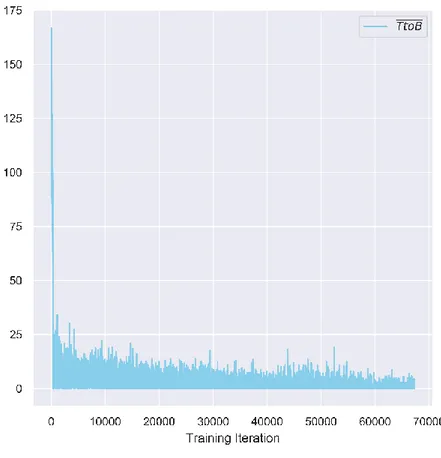
29 The evolution of the average inverse of episode duration – time remaining to backtesting – decreases over time, exhibiting very small average durations on the first few hundred iterations, rapidly converging towards 0. These dynamics are consistent with that of an agent which understands the consequences of over-optimizing the short-term reward through very small disclosure, resulting in a bankruptcy state. The statement is compliant with figure 2, where the agent obtained large negative rewards beyond -1. Given the bankruptcy state’s reward corresponds to -1, the fact that for such cases, the agent obtained, on average, rewards smaller than -1, is consistent with the episode duration analysis, as in the latter, the agent steers away from the minimal episode duration, thus accumulating increasingly negative rewards, which are added to the final state – bankruptcy – thus yielding a reward smaller than -1.
Figure 3 - The training process’ average time remaining to backtesting, or inverse episode duration as a function of training iterations.
30 4.2.3 Policy Analysis
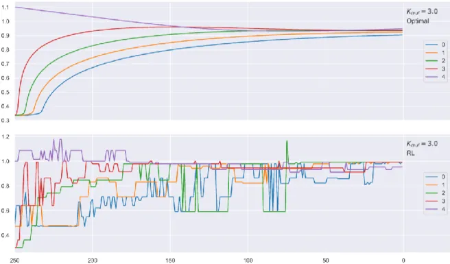
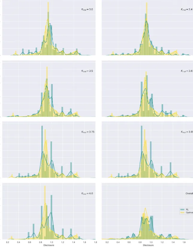
Given the produced policy is sub-optimal and has high variance, both of which, were expected, direct policy interpretation via graphs is not relevant, as a smooth policy was not learnt – see figure 6 and its discussion – and does not constitute this thesis’ goal. Yet, and despite the simulated benchmark to be performed in the next chapter, the current chapter compares each policies’ statistical indicators, to assess to what extent their outline differs.
Disclosure RL DP Mean 0.955 1.016 Standard deviation 0.248 0.439 IQR 0.184 0.201 𝑄1 0.832 0.860 𝑄3 1.016 1.061
Table 4 - The main statistical indicators for the reinforcement learning and dynamic programming policy’s disclosure, where 𝐼𝑄𝑅, 𝑄1 and 𝑄2 represent, the interquartile range, first and third quartiles, respectively.
The disclosure is measured in the interval ]0, 3] in accordance with equation (34).
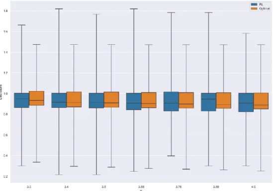
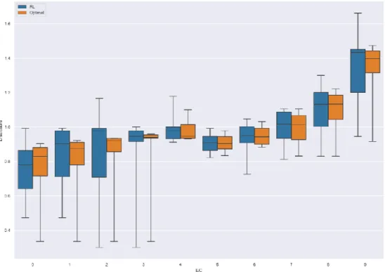
An initial comparison between each policies’ key statistical indicators suggests that the reinforcement learning policy reports, on average, lower percentages of the value-at-risk, regarding its counterpart, considering the entire policy. The artificial intelligence (AI) policy’s statistical indicators exhibit smaller standard deviation and interquartile-range. The optimal policy’s first quartile is larger than its AI counterpart, suggesting a less conservative behavior on the dynamic programming strategy, which is then compensated via higher disclosures, leading to a larger policy mean. Except for the last statement, these findings correspond to the opposite of the expected behavior. The previous table creates an illusion that the policy has converged, especially when combined with figure 4. The remainder of the current chapter will focus on explaining these results, and how they correlate with mean estimation convergence – typically referred to as convergence in mean – so as to unveil the actual convergence extent.
![Figure 2 – The training process’ average scaled rewards to the interval [-1, 0] as a function of training iterations](https://thumb-eu.123doks.com/thumbv2/123dok_br/18080146.865452/34.892.163.743.726.1105/figure-training-process-average-interval-function-training-iterations.webp)