MODELLING OF DAMAGE AND
FRACTURE OF ADVANCED
COMPOSITES
by
Ant´
onio Rui Melro
A Thesis submitted for the degree of Doctor of Philosophy of the University of Porto
ABSTRACT
With the boom of the information age, the doors to novel techniques and more intensive computational processes have opened wide. What yesterday was impossible to achieve, today is becoming a reality. Concepts such as multiscale modelling, merging the worlds of macro- and micromechanics, are establishing themselves as viable alternatives to experimental procedures in the characterisation of the mechanical behaviour of complex materials.
Advanced composite materials are a perfect field for application of such modelling concepts. At the micro-scale level, composites exhibit two distinct phases – the fibrous reinforcements and the matrix resin. The fibres provide strength and stiffness while the matrix gives lateral support to the fibres. Micromechanics provides the means to analyse the constitutive behaviour of each of these constituents and study the influence of each one in the overall mechanical properties of the composite.
This thesis provides new tools for the micromechanical study of com-posite materials. An algorithm to generate a random distribution of fibres with a high fibre volume fraction is developed. The algorithm is statistically verified for the randomness of its results. The generated distributions are used to develop representative volume elements of real composite materials at the micro-scale.
The concept of periodic boundary conditions is applied throughout the thesis. This type of boundary conditions forces the continuity of the material in opposite faces of the representative volume element, as well as the conti-nuity of the displacement field. Results from the micromechanical analyses are submitted to volumetric homogenisation to obtain the macromechanical behaviour of the homogenised composite.
A constitutive damage model has been developed for each constituent of the composite. A plasticity model is implemented to simulate the mechanical behaviour of the matrix, based on available experimental evidence. The plasticity model considers pressure dependency and different yield strengths in tension and compression. Both constituents follow damage evolution laws developed in the framework of thermodynamics of admissible processes. The implemented damage laws do not suffer from mesh dependency.
Both constitutive models were implemented in a commercial finite ele-ment software. The algorithms for generation of random distributions and application of periodic boundary conditions, as well as for post-processing results were all implemented in a package of scripts which provides the pos-sibility to execute all required operations in a sequential and automatic way
without the need for user intervention.
Two applications of these methodologies are presented. The first in-volves the use of the implemented subroutines to plot failure envelopes of a uniaxial composite under different loading conditions. Results from the micromechanical modelling are compared with the results of an analytical failure criterion recently proposed for composite materials.
The constitutive damage models developed are also applied to textile composites. A 5-harness satin wet weave is modelled using CAD software and a representative unit-cell of the material is generated. The yarns are modelled using a transversely isotropic damage law while the matrix is con-sidered to follow the elasto-plastic with damage constitutive law developed in this thesis. Different loading conditions are applied and the evolution of damage obtained from numerical analysis is compared with experimental information available in the literature.
RESUMO
Com o eclodir da era da informa¸c˜ao, as portas de novas t´ecnicas e pro-cessos computacionais mais intensivos foram abertas. O que ontem era im-poss´ıvel de atingir, hoje torna-se realidade. Conceitos como modela¸c˜ao em multi-escala, unificando os mundos da macro- e micromecˆanica, tˆem-se es-tabelecido como alternativas vi´aveis aos procedimentos experimentais de caracteriza¸c˜ao do comportamento mecˆanico de materiais complexos.
Materiais comp´ositos avan¸cados s˜ao uma ´area perfeita para a aplica¸c˜ao de tais conceitos de modela¸c˜ao. Ao n´ıvel da micro-escala, os materiais comp´ositos exibem duas fases distintas – as fibras de refor¸co e a matriz. As fibras fornecem a resistˆencia e rigidez enquanto a matriz providencia o apoio lateral `as fibras. A micromecˆanica permite a an´alise do comporta-mento constitutivo de cada um dos constituintes e o estudo da influˆencia de cada um nas propriedades mecˆanicas globais do comp´osito.
Esta tese fornece um conjunto de novas ferramentas para o estudo mi-cromecˆanico de materiais comp´ositos. Foi desenvolvido um algoritmo capaz de gerar uma distribui¸c˜ao aleat´oria de fibras com uma fra¸c˜ao vol´umica el-evada. A aleatoriedade dos resultados gerados ´e estatisticamente compro-vada. As distribui¸c˜oes geradas s˜ao usadas para o desenvolvimento de ele-mentos de volume representativos de materiais comp´ositos `a micro-escala.
O conceito de condi¸c˜oes fronteira peri´odicas ´e aplicado ao longo da tese. Este tipo de condi¸c˜oes fronteira obriga `a existˆencia de continuidade do ma-terial em faces opostas do elemento de volume representativo, bem como a continuidade do campo de deslocamentos. Os resultados das an´alises mi-cromecˆanicas s˜ao submetidas a homogeneiza¸c˜ao volum´etrica de modo a obter o comportamento macromecˆanico do material comp´osito homogeneizado.
Um modelo constitutivo de dano foi desenvolvido para cada um dos cons-tituintes do material comp´osito. O comportamento n˜ao-linear da matriz ´e modelado atrav´es de um modelo de plasticidade, escolhido com base em resultados experimentais recentes. O modelo de plasticidade entra em con-sidera¸c˜ao com a dependˆencia `a press˜ao e diferentes tens˜oes de cedˆencia `a tens˜ao e `a compress˜ao. Os modelos constitutivos seguem leis de evolu¸c˜ao de dano desenvolvidas no ˆambito da termodinˆamica dos processos revers´ıveis. ´
E garantido que as leis de dano n˜ao sofrem de dependˆencia do tamanho da malha.
Os dois modelos constitutivos foram implementados num software co-mercial de elementos finitos. Os algoritmos para gera¸c˜ao de distribui¸c˜oes aleat´orias e aplica¸c˜ao de condi¸c˜oes fronteira peri´odicas, bem como para p´
os--processamento de resultados foram compilados num pacote de scripts que oferece a possibilidade de executar todas as opera¸c˜oes de modo sequencial e autom´atico sem necessidade de interven¸c˜ao directa por parte do utilizador. Duas aplica¸c˜oes destas metodologias s˜ao apresentadas. A primeira en-volve o uso das subrotinas desenvolvidas na gera¸c˜ao de envelopes de ru-tura de um material comp´osito uniaxial sob diferentes condi¸c˜oes de carrega-mento. Os resultados da modela¸c˜ao micromecˆanica s˜ao comparados com as previs˜oes de um modelo anal´ıtico de rutura recentemente proposto para materiais comp´ositos.
Os modelos constitutivos de dano desenvolvidos s˜ao tamb´em aplicados a materiais comp´ositos tˆexteis. Um tecido com a geometria de 5-harness satin ´e modelado recorrendo a software CAD e uma unidade-celular representativa do material ´e gerada com base nesse modelo. As fibras tˆexteis s˜ao mode-ladas usando uma lei de dano para materiais transversalmente isotr´opicos, enquanto para a matriz se considera que esta segue a lei constitutiva elasto-pl´astica com dano desenvolvida nesta tese. Diferentes condi¸c˜oes de car-regamento mecˆanico s˜ao impostas e a evolu¸c˜ao de dano obtida atrav´es de an´alise num´erica ´e comparada com a informa¸c˜ao experimental dispon´ıvel na literatura.
R´
ESUM´
E
Avec le boom de l’`ere de l’information, les portes `a nouvelles techni-ques et proc´ed´es de calcul plus intensive ont largement ouvert. Ce qui hier ´etait impossible `a r´ealiser, aujourd’hui, est devenue une r´ealit´e. Des concepts tels que la mod´elisation multi-´echelle, la fusion des mondes de la macro- et micro-m´ecanique, s’´etablissent comme des alternatives viables `
a des proc´edures exp´erimentales dans la caract´erisation du comportement m´ecanique des mat´eriaux complexes.
Les mat´eriaux composites avanc´es sont un domaine id´eal pour l’applica-tion de ces concepts de mod´elisal’applica-tion. Au niveau micro-´echelle, les mat´eriaux composites pr´esentent deux phases distinctes - les renforts fibreux et la trice de r´esine. Les fibres offrent r´esistance et rigidit´e alors que la ma-trice donne un support lat´eral sur les fibres. La microm´ecanique fournit les moyens pour analyser le comportement constitutif de chacun de ces constituants et d’´etudier l’influence de chacun d’eux dans les propri´et´es m´ecaniques du composite.
Cette th`ese propose de nouveaux outils pour l’´etude microm´ecanique des mat´eriaux composites. On a d´evelopp´e un algorithme qui permet de g´en´erer une distribution al´eatoire des fibres avec une fraction volumique ´elev´e. L’algorithme est statistiquement v´erifi´ee pour le caract`ere al´eatoire de ses r´esultats. Les distributions g´en´er´ees sont utilis´ees pour le d´eveloppement des ´el´ements de volume repr´esentantifs des mat´eriaux composites r´eels `a la micro-´echelle.
La notion de conditions aux limites p´eriodiques a ´et´e toujours pr´esente pendent la formulation de cette th`ese. Ce type de conditions aux limites force de la continuit´e de la mati`ere dans les faces oppos´ees de l’´el´ement de volume repr´esentatif, ainsi que la continuit´e du champ de d´eplacement. Les r´esultats des analyses microm´ecaniques sont soumis `a une homog´en´eisation volum´etrique pour obtenir le comportement macrom´ecanique du mat´eriel composite homog´en´eis´e.
Un mod`ele d’endommagement constitutif a ´et´e ´elabor´e pour chacun des constituants du composite. On a utilis´e un mod`ele de plasticit´e pour simuler le comportement m´ecanique de la matrice, fond´ee sur les preuves exp´erimentales disponibles. Le mod`ele de plasticit´e consid`ere la d´ependance `
a la pression et diff´erents limites d’´elasticit´e en traction et compression. Les deux constituants suivent les lois d’´evolution de l’endommagement d´evelopp´e dans le cadre de la thermodynamique des processus admissibles. Les lois d’endommagement qu’on a utilis´ees ne souffrent pas de d´ependance `a l’´egard de la maille.
Les deux mod`eles constitutifs ont ´et´e impl´ement´ees dans un logiciel com-mercial d’´el´ements finis. Les algorithmes de g´en´eration de distributions al´eatoires et d’application des conditions aux limites p´eriodiques, ainsi que de post-traitement des r´esultats ont ´et´e tous mis en œuvre dans un en-semble de scripts qui pr´evoit la possibilit´e d’ex´ecuter toutes les op´erations n´ecessaires de fa¸con s´equentielle et automatique sans avoir besoin de l’inter-vention de l’utilisateur.
Deux applications de ces m´ethodes sont pr´esent´ees. La premi`ere con-cerne l’utilisation des routines impl´ement´ees pour repr´esenter graphique-ment les enveloppes de rupture d’un composite uniaxial sous diff´erentes con-ditions de chargement. Les r´esultats de la mod´elisation microm´ecanique sont compar´es avec les r´esultats d’un crit`ere de rupture analytique r´ecemment propos´e pour les mat´eriaux composites.
Les mod`eles constitutifs d´evelopp´es sont aussi appliqu´es aux composi-tes textiles. Un textile du type 5-harness satin est mod´elis´e en utilisant un logiciel de CAO et une unit´e repr´esentative de la mati`ere est g´en´er´ee. Les fils sont mod´elis´es avec une loi d’endommagement transversalement isotrope alors qu’on consid`ere que la matrice a suivi le comportement ´elasto-plastique avec la loi constitutive d´evelopp´ee dans cette th`ese. Diff´erentes conditions de chargement sont appliqu´ees et l’´evolution d’endommagement r´esultant de l’analyse num´erique est compar´ee avec les informations exp´erimentales disponibles dans la litt´erature.
ACKNOWLEDGEMENTS
I wish to thank the patience and availability of both my supervisors, Prof. Pedro P. Camanho and Prof. Silvestre T. Pinho, who have tried to guide this blind monkey through the mysterious and intertwined paths of the PhD road. It has been a long road, riddled with the most diverse obstacles and Sisyphean tasks. . . But I hope the boat has reached safe harbour now. During the initial stage of development of non-linear models, Prof. Fran-cisco Pires provided a valuable start-up assistance with the understanding of the analytical and numerical pathways necessary to their successful im-plementation.
To Julieta Santos, one of the most tenacious people around me, but without who it would be fairly impossible for me to have reached this level in my life. Thank you for being always close and tender but, most importantly, thank you for giving me my wings.
I express my gratitude towards Funda¸c˜ao para a Ciˆencia e a Tecnologia for awarding me a doctoral degree grant funded by POPH QREN -Tipologia 4.1 - Forma¸c˜ao Avan¸cada, sponsored by Fundo Social Europeu. A reference also to the research grant awarded to me in the last year of doctoral studies from project PDCTE/EME/65099/2003 - Development of failure models and criteria for 5-harness satin weaved composite obtained by RTM.
To my workgroup and peer colleagues, Miguel Bessa, Giuseppe Catalan-otti, Cassilda Tavares, Hannes K¨orber, Hilal Er¸cin, Matthias Vogler, Pedro Martins, Carla Roque, Marco Parente, and Jorge Belinha I thank their friendship, support and valuable discussions throughout this endeavour.
For their invaluable help with all the bureaucratic paperwork and con-tract signing, I thank Mrs. J´ulia Meira, Mrs. Fernanda Fonseca, Mrs. Z´elia Prior and Mrs. Luzia Monteiro.
Not to forget some of the most extraordinary students I was lucky to come across during my PhD years. I will not name any as I might forget some and that would be extremely unfair. It has been an enormous pleasure to have been granted the opportunity to share the little knowledge I have with all these young and bright minds of the future.
To all those whose simple existence has shed light on me in different levels of life, I thank you from the deep ends of my soul, independently of where and how you are in present day.
Abstract i
Resumo iii
R´esum´e v
Acknowledgements vii
Table of Contents ix
List of Symbols xiii
List of Figures xxi
List of Tables xxvii
1 Introduction 1
2 Development of a SRVE 9
2.1 Introduction and state of the art . . . 9
2.1.1 Representative Volume Element . . . 11
2.1.2 Size of a RVE . . . 11
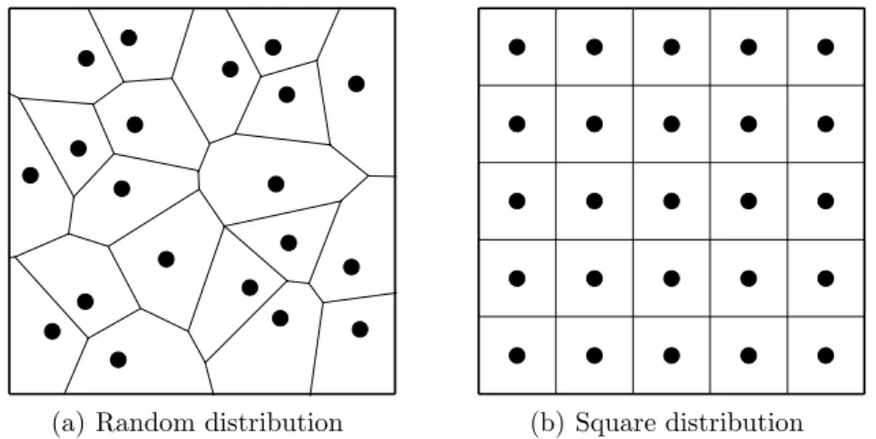
2.1.3 Spatial distribution of fibres inside the RVE . . . 14
2.1.4 Methodologies to generate transverse randomness of reinforcement . . . 17
2.1.5 Statistical spatial descriptors . . . 20
2.1.6 Conclusion . . . 26
2.2 MATLABr script to generate a SRVE . . . 27
2.2.1 Definition of the SRVE . . . 27
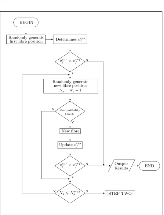
2.2.2 Main flowchart . . . 28
2.2.3 STEP ONE – Hard-core model . . . 30
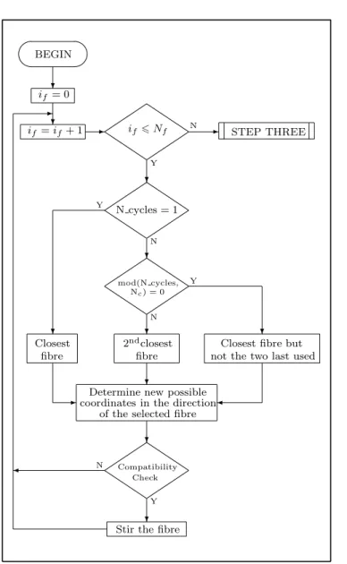
2.2.4 STEP TWO – Stirring the fibres . . . 32
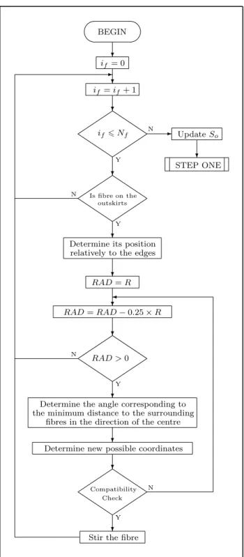
2.2.5 STEP THREE – Fibres in the outskirts . . . 35
2.2.6 Auxiliary functions . . . 38
2.2.7 Examples of generated fibre spatial distributions . . . 39 ix
2.3 Statistical characterisation . . . 46
2.3.1 Time . . . 46
2.3.2 Voronoi polygon areas and neighbouring distances . . 47
2.3.3 Ripley’s K function . . . 48
2.3.4 Pair distribution function . . . 52
2.3.5 Nearest neighbours . . . 52
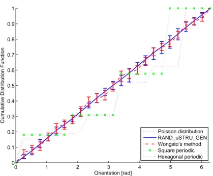
2.3.6 Nearest neighbour orientations . . . 57
2.4 Material characterisation of generated SRVE . . . 59
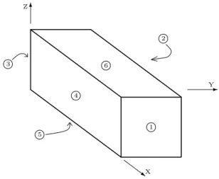
2.4.1 Generated SRVEs . . . 59
2.4.2 Finite element modelling . . . 59
2.4.3 Analyses and Results . . . 62
2.5 Conclusions . . . 65
3 Elastic properties 67 3.1 Introduction and state of the art . . . 67
3.1.1 Effective properties of transverse isotropic materials . 68 3.1.2 Analytical methods . . . 70
3.1.3 Numerical methods . . . 75
3.1.4 Periodic boundary conditions in 3D . . . 80
3.2 Generation of the RVE . . . 84
3.2.1 3D geometry and mesh . . . 84
3.2.2 Definition of PBC’s and pre-processing for FE analysis 86 3.2.3 Obtaining the elastic properties . . . 87
3.3 Comparison of methods . . . 89
3.4 Parametric studies . . . 97
3.4.1 RVE size . . . 97
3.4.2 Fibre radius . . . 100
3.4.3 RVE thickness . . . 100
3.4.4 Minimum gap between fibres . . . 100
3.5 Conclusions . . . 100
4 Plasticity model for epoxy resins 107 4.1 Plasticity theory . . . 107
4.1.1 Additive decomposition of the strain tensor . . . 108
4.1.2 Elastic law . . . 109
4.1.3 Yield function . . . 109
4.1.4 Plastic flow and loading/unloading conditions . . . 110
4.1.5 Hardening law . . . 111
4.1.6 Plastic flow rule . . . 111
4.1.7 Plastic multiplier . . . 112
4.1.8 Elastoplastic tangent operator . . . 113
4.2 Computational plasticity . . . 114
4.3 Plastic response of epoxy polymers . . . 118
4.4.1 Yield surface formulation . . . 125
4.4.2 Flow rule . . . 127
4.4.3 Hardening law . . . 130
4.4.4 Return mapping algorithm . . . 131
4.4.5 Consistent tangent operator . . . 134
4.5 Computational implementation . . . 137
4.6 Verification of elasto-plastic model . . . 140
4.6.1 One-element testing . . . 140
4.7 Application to composite volume elements . . . 141
4.7.1 Transverse tension . . . 141
4.7.2 Longitudinal shear . . . 142
4.7.3 Transverse shear . . . 143
4.7.4 Transverse compression . . . 143
4.7.5 Combined transverse compression and shear . . . 144
4.8 Conclusions . . . 145 5 Damage models 147 5.1 Damage in composites . . . 147 5.1.1 Macro-scale . . . 148 5.1.2 Meso-scale . . . 148 5.1.3 Micro-scale . . . 154
5.1.4 Damage prediction at the micro-level: state of the art 158 5.2 Numerical simulation of damage . . . 165
5.2.1 Crack band model . . . 167
5.2.2 Damage mechanics theory . . . 168
5.3 Definition of damage model . . . 174
5.3.1 Matrix . . . 174
5.3.2 Fibrous reinforcements . . . 183
5.4 Comput. implement. of the damage models . . . 190
5.4.1 Matrix . . . 190
5.4.2 Fibrous reinforcements . . . 192
5.4.3 Determining the damage parameters . . . 193
5.5 Verification of the damage models . . . 196
5.5.1 One-element testing . . . 196
5.5.2 Open-hole tensile tests . . . 199
5.6 Application to composite volume elements . . . 204
5.6.1 Transverse tension . . . 204
5.6.2 Longitudinal shear . . . 205
5.6.3 Transverse shear . . . 206
5.6.4 Transverse compression . . . 206
5.6.5 Combined transverse compression and shear . . . 207
5.6.6 Longitudinal tension . . . 208
6 Failure envelopes 211
6.1 Analytical model . . . 211
6.2 Failure envelopes . . . 215
6.2.1 Biaxial transverse load . . . 216
6.2.2 Transverse normal and longitudinal shear load τ12 . . 218
6.2.3 Transverse normal and longitudinal shear load τ13 . . 220
6.2.4 Transverse normal and transverse shear load . . . 222
6.3 Conclusions . . . 224
7 Application to textile composites 225 7.1 Different types of textile composites . . . 226
7.2 State of the art on 5-harness satins . . . 229
7.3 Generation of representative volume element . . . 234
7.3.1 Geometry of weave . . . 234
7.4 Periodic boundary conditions . . . 238
7.5 Constitutive models . . . 240
7.6 Elastic and strength properties of yarns . . . 242
7.7 Numerical study of 5-harness satin . . . 244
7.7.1 Uniaxial tension . . . 245
7.7.2 In-plane shear . . . 245
7.7.3 Biaxial tension . . . 248
7.7.4 Uniaxial tension and in-plane shear . . . 248
7.8 Conclusions . . . 251
8 Conclusions and future work 253 8.1 Achievements . . . 253 8.2 Improvements . . . 256 8.3 Future Work . . . 258 8.3.1 Multiscale analyses . . . 258 8.3.2 Distributed computing . . . 259 Bibliography 262
A MATLABr script for RAND uSTRU GEN 277
B MATLABr script for pre-processing 279
C FORTRAN code with plasticity model 281
D UMAT with both constitutive models 283
Chapter 2
a Representative volume element size
Ei Young’s modulus in i-direction
g(h) Pair distribution function
Gij Shear modulus in ij-plane
if Counter of number of fibres in algorithm RAND uSTRU GEN
k Random factor between 0 and 1 in Wongsto’s
perturbation process
K(h) Ripley’s K function
b
K(h) Estimate of Ripley’s K function
KH(h) Ripley’s K function for a hard-core point pattern KP(h) Ripley’s K function for a Poisson point pattern b
L(h) Difference between bK(h) and KH(h)
Nc Number of iterations before changing criterion in step two of algorithm RAND uSTRU GEN
Nf Number of fibre positions generated by RAND uSTRU GEN Ng Current number of attempts of fibre placement in step one
of algorithm RAND uSTRU GEN
Ngmax Maximum number of attempts of fibre placement in step one of algorithm RAND uSTRU GEN
Ni Current number of iterations in algorithm RAND uSTRU GEN Nmax
i Maximum number of iterations the algorithm
RAND uSTRU GENis allowed to execute
R Fibre radius
So Initial square size in step three of RAND uSTRU GEN
S+ Increment to be given to square size in step three of RAND uSTRU GEN
vf Fibre volume fraction
vcurf Current fibre volume fraction in RAND uSTRU GEN vreqf Requested fibre volume fraction for RAND uSTRU GEN δ Ratio of representative volume element size to fibre radius
∆min Minimum distance between fibres
ε Strain tensor
θw Direction of displacement in Wongsto’s perturbation process
νij Poisson’s ratio
ν(x) Average of variable x
ρ(x) Coefficient of variation of variable x
ρA Coefficient of variation of areas of Voronoi cells ρD Coefficient of variation of neighbouring distances
ρw Maximum distance in Wongsto’s perturbation process
σ Stress tensor
σ(x) Standard deviation of variable x
2D 2-Dimensional
3D 3-Dimensional
CDF Cumulative Distribution Function
CFRP Carbon Fibre Reinforced Polymer
CMC Ceramic Matrix Composite
FEA Finite Element Analysis
MMC Metal Matrix Composite
PBC Periodic Boundary Conditions
PDF Probability Density Function
RVE Representative Volume Element
SRVE Statistical Representative Volume Element Chapter 3
a Width of representative volume element
b Height of representative volume element
c Thickness of representative volume element
C Stiffness tensor
Cijkl Stiffness tensor in Voigt notation
Cijklf Stiffness tensor of the fibre in Voigt notation Cijklm Stiffness tensor of the matrix in Voigt notation
Ei Young’s modulus in i-direction
Ef Young’s modulus of isotropic fibre material
Em Young’s modulus of isotropic matrix material
Gij Shear modulus in ij-plane
Gf Shear modulus of isotropic fibre material
Gm Shear modulus of isotropic matrix material
k23 Plain strain bulk modulus
kf Plain strain bulk modulus of isotropic fibre material km Plain strain bulk modulus of isotropic matrix material
K Bulk modulus
Km Bulk modulus of isotropic matrix material
S Compliance tensor
Sijkl Compliance tensor in Voigt notation
Sijklf Compliance tensor of the fibre in Voigt notation Sm
ijkl Compliance tensor of the matrix in Voigt notation
uni Degree of freedom i of node n
V Volume of representative volume element
Vf Fibre volume fraction
Vm Matrix volume fraction
W Strain energy density function
ε Strain tensor
εij Strain tensor in Voigt notation
εo Far-field strain tensor
νij Poisson’s ratio
νf Poisson’s ratio of isotropic fibre material νm Poisson’s ratio of isotropic matrix material
σ Stress tensor
σij Stress tensor in Voigt notation
2D 2-Dimensional
3D 3-Dimensional
API Application Programming Interface
CCA Composite Cylinder Assemblage model
FEA Finite Element Analysis
Hashin+ Upper Bound of Hashin’s model
Hashin- Lower Bound of Hashin’s model
MMC Metal Matrix Composite
PBC Periodic Boundary Conditions
RVE Representative Volume Element
StMat Strength of Materials model
Chapter 4
De Elastic stiffness tensor
Dep Elastoplastic tangent operator Ei Young’s modulus in i-direction Eep Elastoplastic tangent modulus g Non-associative flow potential
G Elastic shear modulus
H Generalised hardening modulus
I Second order identity tensor I1 First invariant of stress tensor Itr
1 First invariant of trial stress tensor
Jtr
2 Second invariant of deviatoric trial stress tensor
K Elastic bulk modulus
N Flow vector
p Hydrostatic pressure
ptr Hydrostatic component of trial stress tensor q Set of variables affected by hardening S Deviatoric stress tensor
Str Deviatoric trial stress tensor
α Hardening variables
γ Plastic multiplier
∆x Increment of variable x
ε Strain tensor
εtr Trial strain tensor εe Elastic strain tensor
εed Deviatoric component of elastic strain tensor εe
v Volumetric component of elastic strain tensor εp Plastic strain tensor
εpd Deviatoric component of plastic strain tensor εpe Equivalent plastic strain
εpv Volumetric component of plastic strain tensor νij Poisson’s ratio
νp Plastic Poisson’s ratio
σ Stress tensor
σo Uniaxial yield stress σc Compressive yield stress σs Shear yield stress σt Tensile yield stress σvm Von Mises stress σtr Trial stress tensor
Φ Yield surface
Ψ Flow potential
Chapter 5
C Damaged stiffness tensor
Cf Stiffness tensor of fibre material
CfT Constitutive tangent operator in damage model for fibre Cm Stiffness tensor of matrix material
CmT Constitutive tangent operator in damage model for matrix
Co Non-damaged stiffness tensor
d Damage variable
df Damage variable in fibre damage model
Ei Young’s modulus in i-direction
Em Non-damaged Young’s modulus of matrix material
Eo Non-damaged Young’s modulus
Fd
f Damage activation function in damage model of fibre
Fmd Damage activation function in damage model of matrix
F I Failure Index
Gij Shear modulus in ij-plane
Go Non-damaged shear modulus
Gf e Fracture energy
Gf f Fracture energy in mode I of fibre material Gf m Fracture energy in mode I of matrix material
Gm Complementary free energy density of matrix damage model
GP
m Complementary free energy density of matrix damage model
associated with plastic flow
Gf Complementary free energy density of fibre damage model
Hf Compliance tensor of fibre material
Hm Compliance tensor of matrix material
Hfo Non-damaged compliance tensor of fibre material Ho
m Non-damaged compliance tensor of matrix material
I Second order identity tensor
I1 First invariant of stress tensor ˜
I1 First invariant of effective stress tensor ˜
J2 Second invariant of effective deviatoric stress tensor
K Bulk modulus
Ko Non-damaged bulk modulus
le Characteristic element length
Q Shear strength in xy-plane
rf Internal damage variable in damage model of fibre rm Internal damage variable in damage model of matrix
R Shear strength in xz-plane
S Shear strength in yz-plane
SL Longitudinal shear strength
ST Transverse shear strength
ui Displacement in i-direction
U Energy required for complete failure of one element
Uv Dilatational energy density
XC Compressive strength in x-direction
XT Tensile strength in x-direction
XfT Uniaxial tensile strength of fibre material XC
m Uniaxial compressive strength of matrix material XmT Uniaxial tensile strength of matrix material
YC Compressive strength in y-direction
Ym Associated thermodynamic force in damage model of matrix YT Tensile strength in y-direction
ZC Compressive strength in z-direction
ZT Tensile strength in z-direction
α Fracture angle under transverse compressive loads
Γij Ultimate shear strain in ij-plane
ε Strain tensor
εeq Equivalent strain
εCij Ultimate compressive strain εTij Ultimate tensile strain
ηL Longitudinal friction coefficient ηT Transverse friction coefficient
Ξf Rate of energy dissipation per unit volume in fibre material Ξm Rate of energy dissipation per unit volume in matrix material
νij Poisson’s ratio
νm Non-damaged Poisson’s ratio of matrix material
νo Non-damaged Poisson’s ratio
σ Stress tensor
˜
σ Effective stress tensor
σn Stress component normal to fracture plane
τL Longitudinal shear component in fracture plane
τT Transverse shear component in fracture plane
φd
f Loading function for damage model of fibre
φdm Loading function for damage model of matrix
Ψ Energy dissipated per unit volume
Ψf Energy dissipated per unit volume in damage model of fibre Ψm Energy dissipated per unit volume in damage model of matrix
BEM Boundary Element Model
OHT Open Hole Tensile geometry
RVE Representative Volume Element
UMAT User subroutine to define a material’s mechanical behaviour in commercial finite element analysis software ABAQUSr
VCCT Virtual Crack Closure Technique
WWFE World Wide Failure Exercise
Chapter 6
Ei Young’s modulus in i-direction
Gij Shear modulus in ij-plane
SL Longitudinal shear strength
SLis In-situ longitudinal shear strength STis In-situ transverse shear strength
YT Transverse tensile strength YTis In-situ transverse tensile strength
α Fracture angle under transverse compressive loads
εo Far-field strain tensor
εT1 Maximum tensile strain in longitudinal direction ηL Longitudinal friction coefficient
ηT Transverse friction coefficient
νij Poisson’s ratio
σ Stress tensor
σφ Stress tensor in rotated reference frame
σI Maximum principal stress on a transverse plane to the fibres σN Normal stress component in fracture plane
τL Longitudinal shear component in fracture plane τT Transverse shear component in fracture plane F F C Failure criterion for fibre compression
F F T Failure criterion for fibre tension
F KM C Failure criterion for matrix compression in rotated reference frame
F KM T Failure criterion for matrix tension in rotated reference frame F M C Failure criterion for matrix compression
F M T Failure criterion for matrix tension Chapter 7
a Width of representative volume element
c Thickness of representative volume element Ei Young’s modulus in i-direction
E◦
i Young’s modulus in i-direction of satin weave
FN Damage activation function in mode N
Gij Shear modulus in ij-plane G◦
12 Shear modulus in 12-plane of satin weave GF CIC Fracture toughness for longitudinal compression GF EIC Fracture toughness in mode I for longitudinal tension,
exponential damage evolution law
GF LIC Fracture toughness in mode I for longitudinal tension, linear damage evolution law
GMIC Fracture toughness in mode I for transverse tension GMIIC Fracture toughness in mode II for transverse shear rN Internal damage variable for failure mode N SL Longitudinal shear strength
un
i Degree of freedom i of node n
XC Compressive strength
XP O Fibre pull-out strength
XT Tensile strength
YC Transverse compressive strength YT Transverse tensile strength
αii Coefficient of thermal expansion in i-direction
ε Strain tensor
εo Far-field strain tensor νij Poisson’s ratio
ν12◦ Poisson’s ratio in 12-plane of satin weave
σo Homogenised stress tensor
˜
σ Effective stress tensor
φN Loading function in mode N
2D 2-Dimensional
CAD Computer Aided Design
PBC Periodic Boundary Conditions
RVE Representative Volume Element
Chapter 8
I1 First invariant of stress tensor
J2 Second invariant of deviatoric stress tensor
J3 Third invariant of deviatoric stress tensor
ε◦P Strain tensor at integration point P at macro-scale
σ◦P Stress tensor at integration point P at macro-scale
BOINC Berkeley Open Infrastructure for Network Computing
CPU Central Processing Unit
GNU Gnu’s Not Unix
GPU Graphics Processing Unit
SETI@Home Search for Extraterrestrial Intelligence at Home
Chapter 2
2.1 Two patterned spatial distributions of reinforcements . . . 15 2.2 Matsuda et al. ’s spatial distributions of reinforcements . . . 16 2.3 Perturbation process proposed by Wongsto and Li . . . 20 2.4 Voronoi cells . . . 21 2.5 Examples of K(h) and g(h) functions by Pyrz . . . 26 2.6 Definition of SRVE regions . . . 27 2.7 Flowchart of algorithm RAND uSTRU GEN . . . 29 2.8 Flowchart of STEP ONE in algorithm RAND uSTRU GEN . . . . 31 2.9 Flowchart of STEP TWO in algorithm RAND uSTRU GEN . . . 33 2.10 Concept behind STEP TWO . . . 34 2.11 Flowchart of STEP THREE in algorithm RAND uSTRU GEN . . 36 2.12 Definition of the outskirts in STEP THREE . . . 37 2.13 Evolution of fibre spatial distribution – sequence 1 . . . 39 2.14 Evolution of fibre spatial distribution – sequence 2 . . . 40 2.15 Evolution of fibre spatial distribution – sequence 3 . . . 41 2.16 Evolution of fibre spatial distribution – sequence 4 . . . 42 2.17 Evolution of fibre spatial distribution – sequence 5 . . . 43 2.18 Evolution of fibre spatial distribution – sequence 6 . . . 44 2.19 Evolution of fibre spatial distribution – sequence 7 . . . 45 2.20 Fibre distributions in analysis with vfreq= 56% . . . 49 2.21 Fibre distributions in analysis with vfreq= 65% . . . 50 2.22 L(h) function for vreqf = 56% . . . 51 2.23 L(h) function for vreqf = 65% . . . 51 2.24 Pair distribution function for vreqf = 56% . . . 53 2.25 Pair distribution function for vreqf = 65% . . . 53 2.26 First nearest neighbour function for vreqf = 56% . . . 54 2.27 First nearest neighbour function for vreqf = 65% . . . 54 2.28 Second nearest neighbour function for vreqf = 56% . . . 55 2.29 Second nearest neighbour function for vreqf = 65% . . . 55
2.30 Third nearest neighbour function for vfreq= 56% . . . 56 2.31 Third nearest neighbour function for vfreq= 65% . . . 56 2.32 Nearest neighbour orientation for vfreq= 56% . . . 58 2.33 Nearest neighbour orientation for vfreq= 65% . . . 58 2.34 Generated SRVEs for transversal isotropy demonstration . . . 59 2.35 Generated triangular mesh . . . 60 2.36 Periodic boundary conditions . . . 61 2.37 Young’s moduli and transverse shear modulus . . . 63 2.38 Poisson’s ratios . . . 64
Chapter 3
3.1 Composite cylinder assemblage model . . . 73 3.2 Unit cell RVEs based on periodic distributions . . . 76 3.3 Rigid boundary conditions . . . 78 3.4 Embedded cell approach . . . 79 3.5 Periodic boundary conditions. . . 80 3.6 Face numbering of RVE for application of PBC . . . 81 3.7 Edge numbering of RVE for application of PBC . . . 82 3.8 Vertex numbering of RVE for application of PBC . . . 83 3.9 Solids for both matrix and fibre set . . . 85 3.10 Final solid with generated random distribution of fibres . . . 85 3.11 Final mesh of generated random distribution of fibres . . . . 86 3.12 Longitudinal Young’s modulus for AS4/3501-6 . . . 90 3.13 Transverse Young’s modulus for AS4/3501-6 . . . 90 3.14 Longitudinal Poisson’s ratio for AS4/3501-6 . . . 91 3.15 Longitudinal shear modulus for AS4/3501-6 . . . 91 3.16 Transverse shear modulus for AS4/3501-6 . . . 92 3.17 Transverse Poisson’s ratio for AS4/3501-6 . . . 92 3.18 Longitudinal Young’s modulus for Silenka/MY750/HY917/
DY063 . . . 93 3.19 Transverse Young’s modulus for Silenka/MY750/
HY917/DY063 . . . 93 3.20 Longitudinal Poisson’s ratio for Silenka/MY750/HY917/DY063 94 3.21 Longitudinal shear modulus for Silenka/MY750/HY917/DY063 94 3.22 Transverse shear modulus for Silenka/MY750/HY917/DY063 95 3.23 Transverse Poisson’s ratio for Silenka/MY750/HY917/DY063 95 3.24 AS4’s effective engineering properties as a function of RVE size 98 3.25 Silenka’s effective engineering properties as a function of RVE
size . . . 99 3.26 AS4’s effective engineering properties as a function of fibre
3.27 Silenka’s effective engineering properties as a function of fibre radius . . . 102 3.28 AS4’s effective engineering properties as a function of RVE
thickness . . . 103 3.29 Silenka’s effective engineering properties as a function of RVE
thickness . . . 104 3.30 AS4’s effective engineering properties as a function of
mini-mum fibre gap . . . 105 3.31 Silenka’s effective engineering properties as a function of
min-imum fibre gap . . . 106
Chapter 4
4.1 Mathematical model of uniaxial tensile test . . . 108 4.2 Return mapping scheme . . . 116 4.3 Results of tensile tests by Fiedler et al. . . 120 4.4 Results of compression tests by Fiedler et al. . . 120 4.5 Results of torsion tests by Fiedler et al. . . 120 4.6 Paraboloidal criterion with experimental data by Fiedler et al. 122 4.7 Paraboloidal yield surface . . . 124 4.8 Flowchart of implicit elastic predictor/return mapping
algo-rithm . . . 137 4.9 Flowchart of return mapping algorithm . . . 138 4.10 Flowchart for improving plastic multiplier’s initial estimate . 139 4.11 Comparison of experimental data with numerical results from
one-element mesh . . . 140 4.12 Results for transverse tension example . . . 142 4.13 Results for longitudinal shear example . . . 142 4.14 Results for transverse shear example . . . 143 4.15 Results for transverse compression example . . . 144 4.16 Results for combined transverse shear and compression example144
Chapter 5
5.1 Puck’s action plane (image from D´avila and Camanho) . . . . 152 5.2 Example of matrix cracks . . . 154 5.3 Interfacial debonding in a HTA/L135i composite . . . 155 5.4 Micrograph showing the fibre pull-out effect on a B/Al
com-posite . . . 156 5.5 Formation of a kink band . . . 156 5.6 Fibre fracture . . . 157 5.7 Single fibre model under transverse compression . . . 161
5.8 Parabolic yield and failure criterion . . . 164 5.9 Mesh-dependency caused by ill-posedness of CDM . . . 166 5.10 Idealised elastic response of damaged material under uniaxial
load . . . 170 5.11 Damage domain for isotropic damaged materials . . . 173 5.12 Flowchart of constitutive model for matrix material . . . 191 5.13 Flowchart of constitutive model for reinforcement material . . 192 5.14 Flowchart of secant method . . . 194 5.15 Flowchart of Simpson’s rule . . . 195 5.16 Example of material law . . . 197 5.17 Stress-strain curves for one-element tests of matrix material . 198 5.18 Stress-strain curves for one-element tests of fibre material . . 198 5.19 Geometry of open-hole tension specimen . . . 199 5.20 Detail of mesh for open-hole tension analyses . . . 199 5.21 Dependence on toughness for epoxy material . . . 200 5.22 Dependence on element size for epoxy material . . . 201 5.23 Dependence on toughness for Carbon fibres . . . 202 5.24 Dependence on element size for Carbon fibres . . . 202 5.25 Dependence on toughness for Glass fibres . . . 203 5.26 Dependence on element size for Glass fibres . . . 203 5.27 Results for transverse tension example . . . 204 5.28 Results for longitudinal shear example . . . 205 5.29 Results for transverse shear example . . . 206 5.30 Results for transverse compression example . . . 207 5.31 Results for combined transverse shear and compression example208 5.32 Results for longitudinal tension example . . . 209
Chapter 6
6.1 Puck’s action plane (image from D´avila and Camanho) . . . . 212 6.2 Misalignment of fibres . . . 214 6.3 Failure envelope for biaxial transverse stresses for Carbon
fi-bre composite . . . 217 6.4 Failure envelope for biaxial transverse stresses for Glass fibre
composite . . . 217 6.5 Failure envelope for transverse normal stress with
longitudi-nal shear τ12 for Carbon fibre composite . . . 219 6.6 Failure envelope for transverse normal stress with
longitudi-nal shear τ12 for Glass fibre composite . . . 219 6.7 Failure envelope for transverse normal stress with
longitudi-nal shear τ13 for Carbon fibre composite . . . 221 6.8 Failure envelope for transverse normal stress with
6.9 Failure envelope for transverse normal stress with transverse shear for Carbon fibre composite . . . 223 6.10 Failure envelope for transverse normal stress with transverse
shear for Glass fibre composite . . . 223
Chapter 7
7.1 Different types of weave patterns . . . 227 7.2 Ishikawa’s idealised mosaic model . . . 229 7.3 Schematic view of Fibre Inclination Model . . . 230 7.4 Idealised angle interlock preform of a satin weave . . . 230 7.5 Model geometry proposed by King et al. . . 231 7.6 Three-dimensional model of plain weave by Zako et al. . . . 232 7.7 Three-dimensional model of 5-harness satin weave by
Daggu-mati et al. . . 233 7.8 Micrograph of 5-harness satin . . . 234 7.9 General dimensions of 5-harness satin weave . . . 235 7.10 Crimp points of 5-harness satin weave . . . 235 7.11 Three-dimensional model for the yarns . . . 236 7.12 Three-dimensional model for the matrix . . . 236 7.13 Assembled model prepared for meshing . . . 237 7.14 Meshed RVE with tetrahedra elements . . . 237 7.15 Detail of the meshed RVE . . . 237 7.16 Face numbering of RVE for application of 2D PBC . . . 238 7.17 Edge numbering of RVE for application of 2D PBC . . . 239 7.18 Results for uniaxial tensile load . . . 246 7.19 Results for in-plane shear load . . . 247 7.20 Results for biaxial tensile load . . . 249 7.21 Results for combination of uniaxial tensile load with in-plane
Chapter 2
2.1 Summary of analysed criteria and results by Trias et al. . . . 14 2.2 Comparison of measured and calculated engineering constants
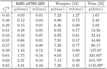
by Gusev . . . 17 2.3 Simulation times to obtain different volume fractions,
accord-ing with Trias’ model . . . 19 2.4 Average and standard deviations of time in minutes required
to run each algorithm . . . 47 2.5 Coefficient of variation for Voronoi polygon areas and
dis-tances to neighbouring fibres . . . 48 2.6 Elastic properties of constituents . . . 60 2.7 Calculated effective properties . . . 62 2.8 Proof of transverse isotropy . . . 62
Chapter 3
3.1 Material properties . . . 89
Chapter 4
4.1 Mechanical properties measured by Fiedler et al. . . 121 4.2 Hardening data measured by Fiedler et al. . . 122
Chapter 5
5.1 Fracture properties . . . 196 5.2 Dimensions of open-hole tension specimen . . . 199 5.3 Parameters used in matrix model verification . . . 200 5.4 Parameters used in Carbon fibre model verification . . . 201
5.5 Parameters used in Glass fibre model verification . . . 201
Chapter 6
6.1 Elastic properties of constituents . . . 215 6.2 Elastic properties of composite systems . . . 215 6.3 Strength properties of composite systems . . . 215 6.4 Definition of loading trajectories . . . 216 6.5 Definition of loading trajectories . . . 218 6.6 Definition of loading trajectories . . . 220 6.7 Definition of loading trajectories . . . 222 Chapter 7
7.1 5-harness satin dimensions . . . 235 7.2 Geometry of the crimp region . . . 235 7.3 Material properties of yarn constituents . . . 242 7.4 Material properties of yarns after homogenisation . . . 243 7.5 Remaining material properties of yarns . . . 243 7.6 Elastic properties of 5-harness satin . . . 244
Introduction
There are two mistakes one can make along the road to truth: not going all the way, and not starting.
Buddha
Composites are regarded as the materials of the future, which will rev-olutionise the industry, help improve environment conditions thanks to the savings they have to offer, provide more safety and easiness of use to different objects and machines, and allow for an even greater number of alternative applications in different fields of engineering.
However, what most people do not realise is that composite materials have in fact been a part of man’s life since the early stages of human civiliza-tion. As a matter of fact, even of man himself. The muscular system of the human body is a perfect example of how the arrangement of multiple fibrous systems can provide strength, versatility and efficiency to a mechanical sys-tem. Indeed, there are in Nature several examples of composite materials. The most obvious and useful to man throughout centuries is undoubtedly wood. Wood is made out of an arrangement of cellulose fibres in a matrix of lignin. The fibres provide tensile strength to the wood while the matrix provides lateral support to the fibres and compressive resistance. And this is the easiest and most common definition of a composite material, taught in every engineering school: a composite is made of two or more constituent materials with different mechanical properties but when put together, each constituent plays a different role in the final mechanical behaviour of the composite.
First evidences of man-made composite materials appear in the cradle of human civilization, when straw and mud were burnt together to form bricks for construction purposes [1]. The technique was used by the Israelites in the Middle East for their Egyptian rulers and is described in the Book
of Exodus. In the same epoch, for the manufacture of papyrus sheets for writing, ancient Egyptians stripped the stem of the papyrus plant into thin but long strips. These strips were then laid side by side. Another layer was laid on top of these, but with the fibres of the plant in a perpendicular direction to the first layer. Several layers were added afterwards to provide enough strength and durability to the papyrus papers for writing. Thus, the first orthotropic laminates were born, out of the simple human need to express itself. . .
Throughout the centuries, there was no strong reason for man to ded-icate much of his time and ingenuity into improving the manufacture and applicability or explore all the potential that composite materials have to offer. Only after the industrial revolution and the growing need for stronger materials, engineers started looking again at combining different materials to obtain better overall mechanical properties. It was in the mid 1800’s that the first attempts at creating a new building material capable of withstand-ing greater stresses began to take place. Joseph Louis Lambot found that the strength of the concrete could be increased by adding to it in its wet state thin bars of steel. Different companies attempted to develop a pro-duction process for this idea, but only in 1878 the first patent was issued, giving rise to the use of reinforced concrete in civil engineering. This new material quickly achieved high popularity since it brought to architecture and civil engineering the possibility to build higher while reducing material weight and increasing longevity of the constructions.
Advanced composite materials as they are known today began gaining shape in 1930 when almost by accident an engineer began wondering about a fibre which formed while applying lettering to a glass bottle [2]. Fibre glass began being manufactured and commercialised first as an insulation material, but soon after it began being applied in the quickly growing aero-nautic industry, first in reinforced plastic dies for manufacture of prototype components, and later in jigs and fixtures for forming and holding aircraft sections and assemblies.
World War II provided the opportunity for the development of many components made of composite materials in the naval and aeronautic indus-try. A significant boost was given in the knowledge of polymers reinforced with fibre glass, their manufacture processes and applications. After the War, the composite industry began looking at different markets where the accumulated knowledge could be applied. The growing automobile industry provided the perfect field for commercial exploration of these materials.
The beginning of the space age in the 1950’s brought the ultimate thrust for the development of advanced composite materials. In 1961 the first patent for production of carbon fibres was issued and soon after carbon fibres
began being commercially available. This allowed for even greater stiffness to weight reductions. New, better, lighter, and stronger components for the aerospace industry began to appear along with new manufacturing processes such as the filament wounding technology. Boron and aramid fibres were respectively introduced in the late 1960’s and early 1970’s.
Not only the fibrous reinforcements suffered a significant evolution; new polymers were also introduced throughout the years allowing for the number of application fields of composites to increase tremendously, expanding from aerospace industry to sports equipment, medical apparatus, defence systems, thermally and chemically demanding environments, and electrical/electronic equipment. And to think it all began with simple mud and straw. . .
Throughout these years of growth in the composite industry, the only procedure to determine whether a given material or component was struc-turally fit to meet the needs was experimentation. The component needed to be manufactured and tested – most of the times to complete destruction – in order to determine its elastic and strength properties. Analytical methods were limited in their application and computers available at the time were not capable of performing advanced calculus in an acceptable time frame.
The computer age which began in the 1990’s provided a magnificent tool for designers and engineers to model parts, components, assemblies, and structures to a level of detail where experimental data is only required for material characterisation purposes, leaving all the iterative process of part development and geometry optimisation to numerical analyses.
Macromechanical analysis is the easiest to perform and the one which requires less computational effort. It allows the designer to study stress patterns and stress concentration regions in the component assuming the composite to be an homogeneous material. Several failure criteria have been proposed throughout the years which can be applied at this level of analyses. The finite element method is seldom used in order to model the mechanical behaviour of the components.
A more detailed study can be performed with mesomechanical analysis. At this level, the mechanical behaviour of a lamina is modelled using con-stitutive material models which still consider the lamina as an homogeneous material. Computational effort is not very high and a more profound study of different damage mechanisms can be performed.
Thanks to the most recent advances in computer technology, network computing and distributed computing, a new level of analysis is rapidly gaining importance and making a stand for itself. Micromechanical analysis looks upon the behaviour of each constituent of the composite, i.e. the
com-posite is seen as an heterogeneous material. Although computationally more expensive, it allows the analyst to have a good overview on the influence of each constituent in the mechanical behaviour of the composite. All kinds of damage mechanisms can be recreated at this level of analysis.
Thanks to numerical homogenisation techniques, the stress and strain fields acquired with micromechanical analyses can provide the constitutive behaviour of the lamina, or even of the laminate. If each of the constituents of the composite is modelled with a physically sound constitutive model, the composite’s elastic, strength, and eventually non-linear properties can be fully determined.
Multi-scale analyses can be performed by using the best out of each level of analysis; meso- or macromechanical analyses provide far-field strain fields on each integration point while the stress field is computed through homogenisation techniques of micromechanical analyses results.
Thesis motivation
Most of the constitutive models presented to date which attempt to simu-late the mechanical behaviour of the composite suffer from a predicament: they are not suited for prediction of the non-linear behaviour of the com-posite, namely under transverse shear, longitudinal shear, and transverse compression, or combinations of different loads.
Being able to predict the non-linear behaviour in composite materials under different loading conditions would allow analysts, designers and engi-neers to harness most of the features which still make advanced composites such a tantalising material to dimension and analyse in the most diverse applications. This non-linear behaviour of the composite is associated with one of the constituents – the matrix.
A possible approach to tackle this problem is by developing a continuum damage model for the matrix material which can be applied in a representa-tive volume element of the microstructure of the composite. This represen-tative volume element should be statistically equivalent to the real material and be able to represent the random distribution of reinforcements that is visible in micrographies of the transverse cross-section of the composite. The representative volume element needs to be loaded under the most general three dimensional strain state so that the influence of the different loading schemes and non-linear and damage mechanisms can be properly studied.
representa-tive volume elements will need to be post-processed using homogenisation techniques in order to obtain the true non-linear behaviour at the lamina level. With the mechanical behaviour of the lamina properly characterised, it is possible to compare the results of the model with available experimental data and other analytical and/or numerical methods to estimate elastic and strength properties of the composite.
There are several limitations on what can be achieved with experimen-tal work. Some loading conditions are extremely difficult to obtain or even impossible given the geometry of the test specimens. Thus, many analyti-cal models for strength prediction can not be validated using experimental data. Three dimensional micromechanical analyses along with homogenisa-tion techniques can provide very detailed and realistic informahomogenisa-tion for any loading condition, allowing for a complete validation of any analytical model. Micromechanical analyses, given the very detailed insight it is capable of providing on the influence of each constituent on the overall mechan-ical behaviour of the composite, will allow for a better understanding of the sequence of events from damage initiation to ultimate fracture of the composite. This knowledge can later be used to attempt to control how a specific damage mechanism is triggered, minimise its hazardous effects and extend the life of the structural component.
Reducing the need for extensive and prolonged experimental work can also be achieved thanks to micromechanical analyses. Considerable cost, material and time savings can be obtained if the micromechanical models are capable of reproducing the results commonly obtained only via experimental procedures.
Thesis objectives
Given the current state of the art in micromechanical analyses of unidirec-tional long-fibre reinforced composite materials, this thesis aims at address-ing the issues of how to generate a representative volume element of the real material and, with the application of adequate boundary conditions, perform micromechanical numerical analyses on it.
The representative volume element will distinguish the two constituents of the composite material – matrix and fibre. Each constituent will have its mechanical behaviour modelled using a thermodynamically sound constitu-tive model, capable of harnessing both linear and non-linear behaviour.
constitutive models in an implicit finite element scheme and apply them to the generated representative volume elements. Results will be put through a volumetric homogenisation process, thus achieving knowledge about the failure strength as well as about which damage mechanisms are associated with each loading scenario. This methodology should be easily reproducible and implemented in other types of composite materials, such as woven com-posites.
Thesis layout
The thesis has been structured so that each chapter approaches one different topic. Care was taken so that this work could be followed and understood by both experienced and untrained readers. Each chapter begins with a review of the state of the art on the subject the chapter is dedicated to, followed by a short but elucidative theoretical introduction to the concepts necessary for the development of the analytical or numerical models presented.
Chapter 2 presents a new algorithm capable of generating a statistically equivalent random distribution of reinforcements with a high fibre volume fraction in a very short period of time. The algorithm is validated using an array of statistical tools and numerical analyses. This algorithm allows for the generation of representative volume elements in three dimensions. How the finite element model can be created, including the application of three dimensional periodic boundary conditions, is presented in chapter 3. A sequence of numerical analyses on different generated distributions is per-formed in order to estimate the elastic constants of a composite material after homogenisation of the stress and strain fields obtained from the mi-cromechanical analyses. A batch of parametric studies is also conducted in order to determine the influence of some geometrical parameters.
The constitutive model for an epoxy resin begins being developed in chapter 4. A plasticity model based on an experimental characterisation of an epoxy resin is implemented in a commercial finite element software. The model is capable of acquiring the most significant properties of an epoxy resin, such as different tensile and compressive yield strengths and pressure dependency. The implemented plasticity model was verified and validated using a sequence of loading conditions applied to different representative volume elements.
The constitutive model of an epoxy resin is completed in chapter 5 with the implementation of an isotropic damage model. This formulation has been developed with the aid of a crack band model capable of inducing mesh independency to the results obtained. Also the reinforcing material was the
subject of development and implementation of a simple mesh-independent transversely isotropic damage model. Both damage models were validated for mesh independency. A similar sequence of analyses on different volume elements that had been performed in chapter 4 is executed here.
With the development of two constitutive models for each of the com-posite’s constituents – matrix and fibre – it is now possible to perform full micromechanical analyses for complete numerical characterisation of a given composite system. Different failure envelopes are outlined in chapter 6, some of them almost impossible to obtain through experimental work, and the re-sults compared with a three dimensional analytical damage model recently proposed.
Finally, in chapter 7 an application of the presented concepts to a tex-tile composite is made. The constitutive damage model developed for the matrix is used on the embedding matrix of the textile, while the yarns are characterised using identical procedures to those in chapter 6 to determine the elastic and strength parameters. These properties are then fed to a transversely isotropic damage model previously developed.
The thesis wraps up in chapter 8 with a summary of achievements, sug-gestions for improvements on the presented methodologies and applications, and a discussion on possible follow-up work in the field of micromechanics using distributed computing.
Development of a
Statistically
Representative Volume
Element
What we call random is just patterns we can’t decipher.
Chuck Palahniuk
When diving into the micro-scale world of heterogeneous materials, there exist two possibilities to numerically model a part’s mechanical behaviour: to mesh the complete part and all of its constituents or to consider the existence of a sufficiently small but representative volume element of the material at hand. While the first option is clearly out of question due to considerably high human and computational effort on meshing and analysis, the latter has been the subject of thorough studies as it provides a method to quantitatively characterize the material’s mechanical behaviour without demanding for an exaggerated computational effort.
This chapter addresses some of the questions related with the appli-cation of the Representative Volume Element (RVE) concept to long fibre reinforced composites, its dimension, generation and statistical equivalence with the bulk material.
2.1
Introduction and state of the art
The mechanics of laminated composite materials can be tackled at three different scales, depending on the problem at hand [3]–[6]:
Micro-scale – This is the scale of the heterogeneity in the com-posite. The mechanical behaviour of the two constituents (fibre and matrix) is the main focus of the analyses per-formed at this scale. The interaction between constituents and the resulting behaviour of the composite (micro-strain and -stress fields) is the main concern of this scale level. Both constituents are seen as individual homogeneous ma-terials. Micro-crack initiation and debonding between fibre and matrix can be easily modelled at this scale. One can also study the effects on the laminate’s strength and stiff-ness of each individual constituent’s properties.
Meso-scale – The scale of the ply thickness. The ply is taken as the building block of the composite, being considered as an homogeneous material with transverse isotropy in the case of unidirectional long fibre composites. The ply me-chanical and elastic properties can be determined through experimentation, but modelling at this scale does not pro-vide any information about the interaction between con-stituents. However, this scale can be much more easily ap-plied to the analysis of large structures than the micro-scale as it does not demand too much computational effort. De-lamination is normally predicted using this scale-level. Macro-scale – The laminate and the structure are at this scale
level. The material is assumed homogeneous and the effects of the constituent materials are represented only by aver-aged apparent properties of the composite material.
Although the meso- and macro-scale material properties can be deter-mined experimentally, it is of interest to establish a relation between the macro-scale mechanical behaviour and the constituents’ properties. This would allow considerable savings on experimental craft and work and pro-vide a deeper knowledge about the real composite’s behaviour leading to a more efficient tailoring of the laminates’ properties according to the engi-neers’ needs for a given application.
However, taking into account all the variables to be considered, perform-ing a thorough analysis at the micro-scale level would be a nearly impossible task. To overcome this difficulty, the concept of statistically homogeneity is normally used [7]. It is considered that there exists a statistical homo-geneous material with the same average properties (like stress and strain) as the heterogeneous material. Calculations can then be performed in this statistically equivalent material.
Assuming that there exists a scale-level for which the properties can be averaged and that this scale is small compared with the real laminate or structure dimensions, one can perform analysis on the material’s re-sponse with reasonable computational effort and still consider the inter-actions between the constituents and their influence on micro-stress (and micro-strain) fields, micro-crack initiation, fibre-matrix interfacial damage, etc. This scale-level is known as a Representative Volume Element (RVE).
2.1.1 Representative Volume Element
The mechanical behaviour of heterogeneous materials can be described at an intermediate scale level by a Representative Volume Element (RVE). The first definition of a RVE dates back to 1963 when Hill [8] defined the concept as a microstructural sub-region that is representative of the entire microstructure in an average sense. The RVE must be [8]:
(a) structurally representative of the mixture of constituents on average, and (b) contain a sufficient number of inclusions for the apparent overall moduli to be effectively independent of the surface values of traction and displacement, as long as these are ‘macroscopically uniform’ .
Drugan and Willis [9] use in their work a slightly different definition for RVE:
the smallest material volume element of the composite for which the usual spatially constant “overall modulus” macroscopic con-stitutive representation is a sufficiently accurate model to repre-sent mean constitutive response.
These definitions refer to an ideal infinite length RVE and so can not be used in computational mechanics. It is thus required to find a finite dimension for the RVE. Different approaches have been suggested in the literature. Some of the most relevant are presented in subsection 2.1.2.
2.1.2 Size of a RVE
The RVE can not have a too large dimension as that would endanger the possibility to numerically analyse it; however, it can not be too small either as this would jeopardise its representativeness of the material in analysis.
Using their definition of RVE, Drugan and Willis [9] demonstrated that the minimum RVE size needs to be at most twice the reinforcement diameter for any reinforcement volume fraction and for several sets of matrix and reinforcement moduli. Although this is computationally attractive, it should be kept in mind that only the global bulk properties were analysed. No attention was given to micro-stress and micro-strain distributions in the RVE nor the effects of a non-linear constitutive model were studied.
Shan et al. [10] studied the micro-structure of a Ceramic Matrix Com-posite (CMC) with random distribution and size of the reinforcement. The study made use of a digital-image analysis process [11] by which the rein-forcement’s spatial distribution would be statistically characterized using six parameters. A computer simulation of hard-core random fibre arrangement was then generated making use of those six parameters, creating fibre-rich and -poor regions which would have a statistically equivalent spatial distri-bution to the real material. They concluded that a window of approximately 40 times the average fibre radius for a volume fraction of 35% represented both geometrically (using a set of statistical functions to quantitatively eval-uate the fibre distribution) and mechanically (through the analysis of the distribution of maximum principal stress on the matrix) the constitutive behaviour of the material. It should be noted though that the constituents’ elastic moduli presented a ratio of 2.3 : 1. This is not the case for CFRP where ratios of 60 : 1 between the constituents’ elastic moduli are common. Swaminathan et al. presented a two-part study on a polymeric matrix reinforced with steel fibres [12]–[13] where in the first part the size of an SRVE1 for unidirectional composite materials without damage was accessed, while in the second part, the same study was conducted but considering interfacial debonding. By using various statistical functions of geometry, stresses, and strains, the authors concluded that, just by including damage, the size of the SRVE had to be doubled in order to maintain a good estimate of the effective elastic stiffness tensor. This leads to the conclusion that the size of the SRVE must be determined considering the purpose of the analysis. If a linear elastic analysis is to be performed, the SRVE size can be considerably smaller than for a viscoelastic-plastic analysis with damage, for example.
Gitman et al. [14] demonstrated that the size of the RVE hardly depends on the loading scheme (tension and shear tests were performed) neither it does on a parameter of interest (stress based or stiffness based) judged using a chi-square criterion given by equation (2.1),
1The abbreviation SRVE will be used in this Thesis when there is a statistical
equiva-lence to the bulk material while RVE refers only to the concept of representative volume element.
χ2 = n X i=1 (ai− hai)2 hai (2.1)
where ai is the investigated parameter, hai is the average of ai and n is the number of realisations, i.e. there are n unit cells with the same size but different inclusion distributions. Five unit cells for each volume fraction studied were generated, each having a different spatial distribution of fibres. However, Gitman et al. [14] also concluded that there is a strong depen-dence of the size of the RVE on the material properties of the constituents (like changing stiffness ratio) as well as of the volume fraction of reinforce-ment.
Trias et al. [15] performed a thorough study where the size of a RVE for long fibre reinforced composites was scrutinized. Various mechanical and statistical variables to analyse different sizes of RVEs were used. The functions and variables used as criteria were:
1. Fibre content. 2. Effective Properties.
3. Hill Condition, as defined by equation (2.2).
hσ : εi = hσi : hεi (2.2)
4. Stress and Strain Fields.
5. Probability Density Functions (PDF) of stress and strain in the matrix. 6. Distance distributions.
Trias et al. [15] defined a parameter δ given by equation (2.3),
δ = a
R (2.3)
where a is the RVE edge length and R is the fibre radius. The results of this study are summarised in table 2.1.
Analysing table 2.1 and using equation (2.3) it can be seen that the minimum size for a SRVE is 50 times the fibre radius. This seems to be the most comprehensive study on the field of RVE size for analyses of long fibre reinforced composites made of a carbon fibre and epoxy matrix, the
![Table 2.1: Summary of analysed criteria and results by Trias et al. [15].](https://thumb-eu.123doks.com/thumbv2/123dok_br/19178552.944262/44.892.213.742.252.767/table-summary-analysed-criteria-results-trias-et-al.webp)
![Table 2.2: Comparison of measured and calculated engineering constants by Gusev [21].](https://thumb-eu.123doks.com/thumbv2/123dok_br/19178552.944262/47.892.158.663.265.441/table-comparison-measured-calculated-engineering-constants-gusev.webp)