Vol. 34, No. 04, pp. 1161 – 1174, October – December, 2017 dx.doi.org/10.1590/0104-6632.20170344s20160272
* To whom correspondence should be addressed
A TVD SCHEME FOR 3D UNSTRUCTURED GRIDS
APPLIED TO COMPOSITIONAL RESERVOIR
SIMULATION
B. R. B. Fernandes
1, I. da C. M. Lima
2, E. P. Drumond Filho
2,
J. C. B. de Oliveira
2, F. Marcondes
3* and K. Sepehrnoori
11Center for Petroleum and Geosystems Engineering, The University of Texas at Austin, USA 2Laboratory of Computational Fluid Dynamics, Federal University of Ceará, Brazil 3Department of Metallurgical Engineering and Materials Science, Federal University of Ceará, Brazil
* Corresponding author: Email [email protected]
(Submitted: April 28, 2016; Revised: June 25, 2016; Accepted: August 11, 2016)
Abstract – In reducing the grid orientation effect for the numerical solution of partial differential equations, interpolation functions play an important role when the advective transport of the governing equations is considered. This is due to the fact that, in general, the unknowns are evaluated in the vertices of the elements and such properties must be extrapolated to inner parts of the elements. First-order schemes, such as upwind, are the easiest methods to use for performing the extrapolation of the properties. However, such methods introduce a large amount of numerical diffusion in the solution. A few higher-order interpolation schemes, on the other hand, are capable of providing solutions free of numerical diffusion, increasing the accuracy of the method and reducing the computational efforts required. In this work, we investigate the TVD interpolation scheme for three-dimensional unstructured grids in conjunction with Element-based Finite Volume Method (EbFVM) using four types of elements: hexahedron, tetrahedron, prism and pyramid.
Keywords: Higher-order TVD scheme, Compositional reservoir simulation, IMPEC approach, EbFVM.
INTRODUCTION
Interpolation schemes play an important role when
numerical methods such as finite-volume method are
used. Usually, most of the unknowns are evaluated in the center of each grid block, for structured grids, or in each vertex, for cell-vertex grids. However, in order to compute
advective and diffusive terms it is necessary to extrapolate
these variables from the cell’s center or vertex of the grid to the interfaces of the grid blocks. This is performed through the use of interpolation functions. Unfortunately, accurate interpolation schemes cannot be used arbitrarily for advective dominant problems. The use of high-order
schemes for the advective dominant problems yields spurious oscillations in the solution. In order to overcome this limitation, the use of a Total Variation Diminishing (TVD) scheme can be an alternative option. It is known that TVD schemes can preserve the monotonicity of the solution, hence avoiding spurious oscillations.
Higher-order TVD schemes usually blend the stability of the upwind schemes with the use of higher-order terms
through the use of flux-limiters. Van Leer (1979) developed the first monotonicity preserving flux-limiter. However,
the importance of the TVD in the monotonicity preserving was only discussed later by Harten (1983). Further, Sweby (1984) developed the TVD region for one-dimensional
of Chemical
Brazilian Journal of Chemical Engineering
problems. Several flux-limiters were later introduced and
studied by other authors, such as Roe (1983), Chakravarthy and Osher (1983), Roe (1986) and Koren (1993).
However, the application of these functions for unstructured grids was not straightforward. The Control-volume Finite Element Method (CVFEM) presented by Baliga and Patankar (1980) was used in conjunction with lower-order schemes; they used upwind and exponential schemes. This exponential function, also known as Flow-Oriented Interpolation (FLO), performs the interpolation based on the exponential element shape functions for the element’s average velocity and linear for the normal direction. Prakash (1986) added the source terms evaluation to the original FLO function, giving rise to the FLOS scheme. Later, Maliska (2004) renamed the CVFEM as Element-based Finite Volume Method (EbFVM), since we still have a conservative approach that borrows the idea
of elements and shape functions from the finite-element
method. New interpolation functions were introduced for the EbFVM, mainly for the simulation of skew grids. Hassam et al. (1983) and Schneider and Raw (1986) were
the first authors to propose skew upwind schemes for
two-dimensional problems. Also, Swaminathan and Voller (1992a, 1992b) adapted the streamline upwind Petrov-Garlekin (SUPG) function developed by Brooks and Hughes (1995) from Cartesian to unstructured grids using EbFVM, presenting the streamline upwind control volume (SUCV). Many of those schemes may produce results with second-order accuracy in space, however at the cost of
low numerical stability and possibly downwind influence, which requires a proper treatment, and in general, they are reduced to first order schemes.
Various TVD schemes have been studied and implemented for unstructured grids, such as Bruner and Walters (1995), and Hou et al. (2011, 2012). However, none of those works aimed at the application of TVD in cell-vertex approaches like as EbFVM. Just recently, Fernandes et al. (2013), based on the work of Darwish
and Moukalled (2003), introduced a TVD scheme for 2D unstructured grids for the EbFVM in conjunction with compositional reservoir simulation. Later, Fernandes et al. (2015a) extended the method for solving three-dimensional problems using Hexahedron element grids. In this work, we extend the work presented by Fernandes et al. (2015a) to tetrahedron, prism, and pyramid elements as well as hybrid element grids. This implementation is performed in the in-house compositional reservoir simulator UTCOMP (1990). UTCOMP is an IMPEC-based (Implicit Pressure Explicit Compositional) compositional, multiphase/ multicomponent simulator that can take into account up to four phases developed at The University of Texas at Austin. The EbFVM implemented in the UTCOMP simulator are based on Marcondes and Sepehrnoori (2010), Marcondes et al. (2013) and Santos et al. (2013) for the General Purpose Adaptive Reservoir Simulator (GPAS). In UTCOMP, the implementation for 2D and 3D unstructured grids using the EbFVM and the IMPEC approach are presented in Fernandes et al. (2012) and Araújo et al. (2016). Additionally, IMPSAT (Implicit Pressure and Saturations) approaches (Fernandes et al., 2014; Fernandes et. al., 2015b) and two volume balance based fully implicit approaches (Fernandes, 2014; Fernandes et al., 2016) were implemented for both Cartesian and unstructured grids. In this manuscript, only IMPEC will be considered.
MATHEMATICAL MODEL
The isothermal fluid flow in porous media can be modeled through a material balance equation for each chemical species and constraint equations. The local equilibrium is assumed in order to model the hydrocarbon
properties, amounts and compositions (Chang, 1990).
The material balance equation of each component considering both advection and diffusion transport and assuming multiphase Darcy’s flow is written as
1 1
1
0 ;
1, 2,..,
,
1
np np
i i
ij
j ij j j j j ij c c
j j
b b
N
q
x
k
S
x
i
n n
V
t
=ξ
λ
φ
=ξ
V
∂
− ∇ ⋅
⋅∇Φ +
Κ ⋅∇
−
=
=
+
∂
∑
∑
where nc represents the number of hydrocarbon components, nc+1 refers to the water component, np is the number of
fluid phases,
ij
Κ
is the physical dispersion tensor,k
is the absolute permeability tensor, Ni is the number of molesof the i-th component, ξj and λj represent, respectively, the
molar density and the mobility of the j-th phase, φ is the
formation porosity, xij represents the mole fraction of the
i-th component in the j-th phase, qi is the molar flow rate of the i-th component of a grid block that contains a well, and Vb stands for the bulk volume of the grid block. The
hydraulic potential of a phase, Φj, is given by
Z
P
j j j=
−
γ
Φ
where Pj e
γ
j are the pressure and specific gravity of the phase j, respectively, and Z denotes the depth, which is positive in the downward direction.Local phase equilibrium is assumed between all
hydrocarbon phases in each grid block. In this work, grid block refers to the control volume that is assembled around each vertex of the grid. This condition is represented by the (1)
phase fugacities (f), as follows:
0 ;
1,....,
;
2,...,
j r
i i c p
f
−
f
=
i
=
n
j
=
n
where the superscript r describes the reference phase, and fugacity is a function described by
(
)
ln
;
1,...,
;
2,...,
j
i ij ij c p
f
=
x
φ
i
=
n
j
=
n
In Eq. (4), ∅ij stands for the fugacity coefficient of
the i-th component in the j-th phase. The mole fraction
constraint equation, for each hydrocarbon phase, and the Rachford-Rice equation are given by
1 1
(
1)
1 0 ,
2,..,
;
0
1
(
1)
nc nc
i i
ij p
i i i
z K
x
j
n
K
ν
= =−
− =
=
=
+
−
∑
∑
where zi and Ki are the overall mole fraction and the
equilibrium ratio of the component i, respectively, and υ is
the gas mole fraction in the absence of water.
The calculations associated with phase equilibrium and
PVT properties are conducted using the Peng-Robinson
Equation of State (Peng and Robinson, 1978). It is assumed
that there is no mass transfer between the water and hydrocarbon phases. Therefore, water is not included in the
flash calculations. Further details about this calculation can
be found in Perschke (1988).
The last equation is the volume constraint equation,
which is given by
1
1
n p j jS
==
∑
where Sj denotes the saturation of the phase j.
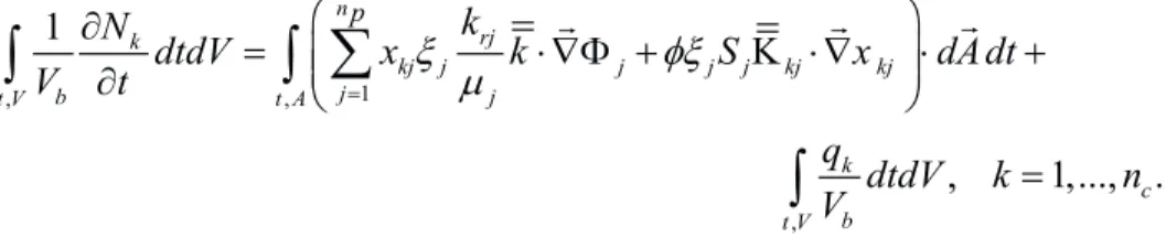
The UTCOMP simulator is based in an IMPEC (Implicit Pressure Explicit Composition) formulation as described by Àcs et al. (1985). The unknown primary variables are the oil pressure and the total number of moles of each component. The oil pressure is obtained from a volume balance, giving rise to the following expression:
0
1 1 1
1
.
n
nc p nc
rj
t k
kj
tk tk
f kj j j j j kj
k j k
b j b
k
V
P
q
c
V
x
k
S
x
V
V
P
t
V
φ
ξ
φξ
µ
= = =
−
∂
∂
=
∇ ⋅
⋅∇Φ + ∇ ⋅
Κ ∇
+
∂
∂
∑ ∑
∑
The applied formulation evaluates the oil pressure implicitly, while all the remaining properties are explicitly evaluated from the previous time step. The mole balance
and flash calculations, for instance, are only conducted
after the pressure at the new time is evaluated.
APPROXIMATE EQUATIONS
In the EbFVM, the physical domain is divided into elements, which are sub-divided into sub-elements according to the number of vertices. These sub-elements are called sub-control volumes, since the material balance
equations are integrated to each one of these sub-elements.
Figure 1 shows the four elements investigated in this work. For each element, a local coordinate system is established.
This allows the simulator to perform the flow rate at each
interface of the sub-control volume, etc. Regardless of how distorted the element is. It is important to stress that except for the pyramid element, the sub-control volumes
of the other three elements always have three quadrilateral
integration surfaces, where the material balance is evaluated; the sub-control volumes of the pyramid element associated to the base have also three integration surfaces, but they are triangular surfaces, and the sub-control volume
associated to apex of the pyramid has 4 quadrilateral
integration surfaces.
In order to obtain the approximate balance equation for each component and pressure, Eqs. (1) and (7) are
integrated in time and for each sub-control of each
element. Integrating, for instance, Eq. (1), in space and
time and applying the Gauss theorem for the advective and dispersion terms, we obtain:
1
, ,
,
1
,
1,...,
.
n
rj k
kj j j j j kj kj j
b j
t V t A
k c b t V p
k
N
dtdV
x
k
S
x
dA dt
V
t
q
dtdV
k
n
V
ξ
φξ
µ
=
∂
=
⋅∇Φ +
Κ ⋅∇
⋅
+
Brazilian Journal of Chemical Engineering
In order to perform the integrations of the first and second terms of Eq. (8), it is necessary to make use of
the shape functions. The shape functions, for hexahedron,
prism, tetrahedron, and pyramid elements, are respectively
given by Eqs. (9) through (12).
(a)
(b)
(c)
(d)
Figure 1. Sub-control volumes for all element types. a) Hexahedron; b) Tetrahedron; c) Prism; and d) Pyramid.
1 2
3 4
5 6
7 8
(1
)(1
)(1
)
(1
)(1
)(1
)
( , , )
;
( , , )
8
8
(1
)(1
)(1
)
(1
)(1
)(1
)
( , , )
;
( , , )
8
8
(1
)(1
)(1
)
(1
)(1
)(1
)
( , , )
;
( , , )
8
8
(1
)(1
)(1
)
(1
( , , )
;
( , , )
8
s
t
p
s
t
p
N s t p
N s t p
s
t
p
s
t
p
N s t p
N s t p
s
t
p
s
t
p
N s t p
N s t p
s
t
p
s
N s t p
N s t p
+
−
+
+
−
−
=
=
−
−
−
−
−
+
=
=
+
+
+
+
+
−
=
=
−
+
−
−
=
=
)(1
)(1
)
8
t
p
+
+
1 2
3 4
5 6
( , , ) (1
)(1
) ;
( , , )
(1
)
( , , )
(1
) ;
( , , )
(1
)
( , , )
;
( , , )
N s t p
s t
p
N s t p
s
p
N s t p
t
p
N s t p
p
s t
N s t p
sp
N s t p
tp
= − −
−
=
−
=
−
=
− −
=
=
, 1 2 3 4( , , ) 1
;
( , , )
( , , )
;
( , , )
N s t p
s t
p
N s t p
s
N s t p
t
N s t p
p
= − − −
=
=
=
, 1 2 3 4 51
( , , )
[(1
)(1
)
/ (1
)]
4
1
( , , )
[(1
)(1
)
/ (1
)]
4
1
( , , )
[(1
)(1
)
/ (1
)]
4
( , , ) [(1
)(1
)
/ (1
)]
( , , )
.
N s t p
s
t
p
stp
p
N s t p
s
t
p
stp
p
N s t p
s
t
p
stp
p
N s t p
s
t
p
stp
p
N s t p
p
=
−
− − +
−
=
+
− − −
−
=
+
+ − −
−
= −
+ − −
−
=
Using the shape functions, the area, volume, and
gradients that are necessary to evaluate each term of Eq. (8),
can be easily evaluated. Further details of this calculation can be found in Marcondes et al. (2013) and Santos et al.
(2013). Adopting an explicit scheme and evaluating the physical properties at each interface of the control volume,
the following expressions for the first and second terms of Eq. (8) are obtained:
, ,
,
;
1,...,
;
1,...,
1
o
m i m m
m i v c
i i
b m
Vscv
N
N
Acc
m
N
i
n
V
t
t
=
−
=
=
+
∆
∆
,
(
)
, 1 30 0 0 0 0 0
1 1
; 1,..., ; , 1,.., 3; 1,..., 1
p
p
n
m i j ij j j j j ij ij
j A
n
j ij
j ij j nl n j j nl n v c
ip j l ip lip
F x K S K x dA
x
x K A S K A m N n l i n
x x
ξ λ φξ
ξ λ φξ
=
= =
= ∇Φ + ∇ =
∂Φ ∂
+ = = = + ∂ ∂
∑
∫
∑ ∑
where ip denotes each integration point located on the surfaces of each sub-control volume and Nv is the number of vertices of each element. A similar procedure is
performed for the pressure equation. Substituting Eqs. (13) and (14) in Eq. (8), the following equation for each
sub-control volume of each element is obtained:
, ,
0 ;
1,...,
;
1,...,
1
m i m i i e c
Acc
+
F
+ =
q
m
=
N
i
=
n
+
.
Brazilian Journal of Chemical Engineering
The above equation stands for the material conservation
for each sub-control volume of each element. The total material balance of each grid volume is computed assembling the contributions of all sub-control volumes that share the same vertex. This procedure is described in detail in Marcondes et al. (2013).
In order to evaluate each term of Eq. (14), it is necessary
to calculate physical properties, such as mole fractions, phase molar densities, and mobilities at the integration points of each sub-control volume. This extrapolation is conducted through interpolation functions. In this work, two interpolation schemes are implemented for the four
element types shown before: a first order upwind, and a second order TVD in conjunction with two flux-limiters.
The upwind interpolation for the EbFVM is analogous to the classic upwind used for Cartesian grids. Considering, for instance, the integration point 1, for all elements shown in Figure 1, the product of physical properties is evaluated by
(
)
,2 ,2 ,21 1
,1 ,1 ,1
1
.
.
0
.
.
0
ij j j j
ip ij j j ip
ij j j j
ip
x
if K
dA
x
x
if K
dA
ξ λ
ξ λ
ξ λ
∇Φ
≤
=
∇Φ
>
.In Eq. (16), the normal to the integration surface
is always positive when it is orientated in the outward direction of that interface.
For the TVD function, we will investigate two
flux-limiters to switch between lower and higher-order schemes. Although the scheme proposed by Fernandes et al. (2013) for approximating the successive slope ratio
has been shown to be efficient for 2D unstructured grids,
results obtained by Fernandes et al. (2014) demonstrated
that, when the gravitational effects are added this scheme is
more prone to spurious oscillations. Therefore, in this work we used the successive slope ratio proposed by Darwish and Moukalled (2003), that performed better than the one used by Fernandes et al. (2013) and Fernandes et al. (2014). According to Darwish and Moukalled (2003), the interpolation of any physical property for the EbFVM can
be evaluated through the following equation:
( )
2
D U f U
r
fδ
= ∆ +
ψ
∆ − ∆
.
In Eq. (17), the subscript f denotes the integration point where the property needs to be evaluated, U denotes the property evaluated in the upwind vertex, D denotes the property evaluated in the downwind vertex, and rf is the successive slope ratio. In this investigation, we will
employ the following equation given by Darwish and
Moukalled (2003) to evaluate the slope ratio:
(
)
(
)
2 U. UD D U
f
D U
r
r = ∇∆ ∆ − ∆ − ∆
∆ − ∆
,
where
∇∆
Urepresents the property’s gradient evaluatedat the upwind vertex, and
∆
r
UD is the vector distance from the upwind node to the downwind node. The gradient at the vertex is evaluated by the volumetric average of the gradient of all elements that share the same vertex (Tran et al., 2006).Finally, the two flux-limiters investigated in this work
for the TVD interpolation function are the MINMOD (Roe, 1986), or MM, as we shall call it from now on, the most
diffusive limiter, and the Koren (1993), a very compressive
limiter. Their expressions are given, respectively, by
MINMOD:
ψ
( )rf =max 0, min 1,(
( )
rf)
,
Koren:
( )
max 0, min 2, 2 ,
2
3
f
f f
r
r
r
ψ
=
+
.
RESULTS
Three case studies will be presented to investigate
the current implementation. The first is an advection-dispersion tracer injection in a quarter of five-spot, the
second case study is a CO2 flooding, and the third case is a CO2 injection in an irregular reservoir. The accuracy of the TVD schemes is presented for each element individually, although the method presented is implemented in a general way and hybrid grids composed of hexahedron, tetrahedron, pyramid or prism can be considered without any further consideration.
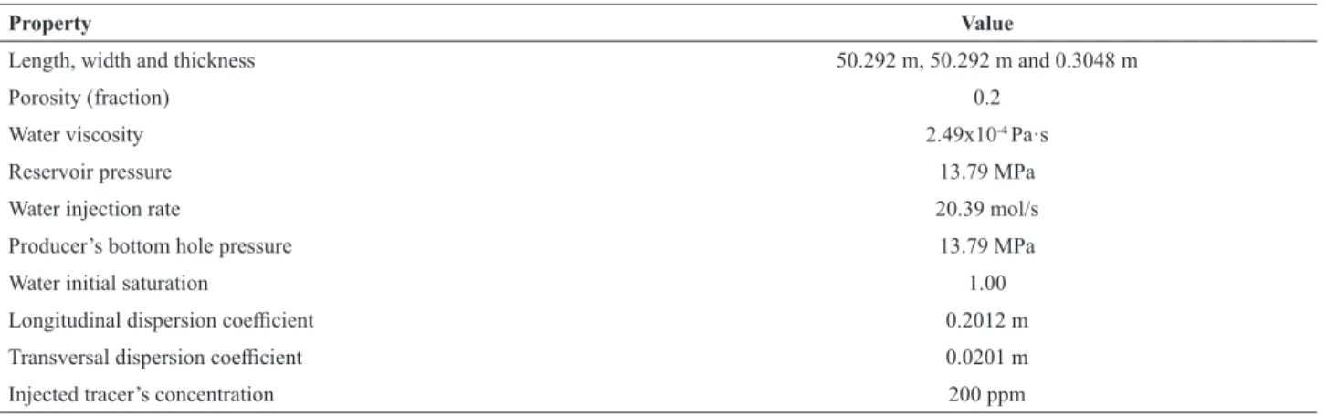
In the first case, a non-reactive tracer is injected in a quarter of five-spot. Water is the only mobile phase and
the tracer does not partition in any other phase other than water. Tracer is injected along with water until a pore volume injected (PVI) of 0.02. After 0.02 PVI, just water
is injected. Gravitational effects are neglected in order to
validate the solutions with the analytical solution given by Abbaszadeh-Dehghani and Brigham (1984). All data for
this case are presented in Table 1. A quarter-of-five spot configuration is used with two vertical wells in the corners.
The grids are formed dividing the reservoir as a Cartesian grid. For elements other than hexahedron, each grid cell is divided again to form the other elements, such as prisms, pyramids, and tetrahedrons.
(16)
(17)
(18)
(19)
The tracer’s effluent profile is presented in Figure 2,
where two grids were used to compare each interpolation function to the exact solution. The results obtained for hexahedron, tetrahedron, prism, and pyramid elements are presented Figures 2a and 2b, 2c and 2d, 2e and 2f, and 2g
and 2h, respectively. As expected, the Koren’s TVD
flux-limiter is always the most accurate while the upwind is less accurate. For the 50x50 grid using hexahedron elements,
the results for the Koren’s flux-limiter were almost in
good agreement with the exact solution. For the grids with tetrahedron elements, the results of the TVD, although accurate, but were not as accurate as for the other elements.
One possible reason for this is the grid orientation effect.
Also, due to the shape functions the tetrahedron is the less accurate element. As can be observed from Figure 2f, the
result obtained with Koren’s flux limiter matches the exact solution. Results presented in Fig. 2h were quite good for
pyramid elements as well.
In the second case study gravity effects are considered.
In this case, CO2 is injected in a quarter of five-spot
configuration. We illustrate this case by running a coarse and a fine grid for hexahedrons, tetrahedrons, and prism elements. The reservoir data and fluid properties for this
case are presented in Table 2. Corey’s model (Corey, 1986) is used for modeling the multiphase relative permeability curves.
The oil and gas volumetric production rate curves are presented in Figure 3. It can be observed that, for the hexahedron and prism element grids, the solution for the upwind scheme converges to the higher resolution schemes
as the grid is refined for both Koren and MINMOD (MM) flux limiters. However, for the tetrahedron element, it can be seen that refining the grid makes the solution
for the upwind scheme deviate from the TVD schemes investigated. The reason for such behavior is that all grids employed in this case study have the same number of vertices in the Z-direction. Since the tetrahedron element is the less accurate element and few vertices in the Z-direction are commonly used in reservoir simulation, the
upwind solutions for the tetrahedron elements have a poor resolution in the Z-direction. As we use the TVD schemes, the resolution in the Z-direction is highly increased and the curves converge to the correct answer. This argument was
confirmed by running more refined grids in the Z-direction,
which resulted in an upwind solution closer to that of the TVD solution.
The gas saturation fields at 260 days for the coarser
grids are presented in Figure 3, where it can observed that the gas saturation front is more dispersed when using the upwind scheme, and less dispersed for MM and Koren’s
flux limiters. This shows how effective the TVD schemes are in reducing the effects of the numerical dispersion.
The third Case is similar to Case 2, but now an irregular reservoir is considered. The reservoir geometry is presented in Figure 5.We used the same data set shown in Table 2, except for the reservoir dimensions. This case shows that a better accuracy can still be obtained when using TVD even if the grid elements are distorted or vary in size. We present the gas production curves in Figure 6. From Figure 6, it can be clearly observed that the upwind curves tend to
that obtained by using Koren’s flux limiter. It also indicates
that the TVD scheme can produce accurate results even for irregular grids.
Figure 6 presents a comparison of the gas saturation field between the upwind and TVD scheme using a Koren flux
limiter, in a plane cut between two of the injecting wells, for the coarser grids at 500 days. This view was chosen
for showing both gravity and displacement effects of the gas saturation front. From this figure, once again it can be observed that the fields obtained with the TVD function
present less numerical dispersion than those obtained with the upwind function. The TVD scheme was not only capable to capture a sharper gas front, but also shows that the gas is expected to migrate to the higher reservoir layers. Such behavior is in accordance to that observed when the
grid is refined in the Z-direction, showing that the TVD
schemes also enhanced the accuracy of the gravitational
effects.
Table 1. Fluid and reservoir data for Case 1.
Property Value
Length, width and thickness 50.292 m, 50.292 m and 0.3048 m
Porosity (fraction) 0.2
Water viscosity 2.49x10⁻⁴ Pa·s
Reservoir pressure 13.79 MPa
Water injection rate 20.39 mol/s
Producer’s bottom hole pressure 13.79 MPa
Water initial saturation 1.00
Longitudinal dispersion coefficient 0.2012 m
Transversal dispersion coefficient 0.0201 m
Brazilian Journal of Chemical Engineering
Figure 2. Tracer concentration in the production well. a) 30x30 hexahedron elements, b) 50x50 hexahedron elements, c) 30x30 tetrahedron elements, d) 50x50 tetrahedron elements, e) 30x30 prism elements, f) 50x50 prism elements, and g) 30x30 pyramid elements, h) 50x50 pyramid elements.
(a) (b)
(c) (d)
(e) (f)
Figure 3. Oil and gas volumetric production rates for each element - Case 2. a) Oil - hexahedron, b) gas - hexahedron, c) oil - tetrahedron, d) gas - tetrahedron, e) oil - prism, f) gas - prism.
(a) (b)
(c) (d)
Brazilian Journal of Chemical Engineering
Figure 4. Gas saturation at 260 days - Case 2. Hexahedron grid with 4410 vertices: a) upwind, b) MM, c) Koren; Tetrahedron grid with 4410 vertices: d) upwind, e) MM, f) Koren; Prism grid with 4410 vertices: g) upwind, h) MM, i) Koren.
Figure 5. Reservoir geometry – Case 3.
(a) (b) (c)
(d) (e) (f)
Figure 6. Gas volumetric production rates for each element - Case 3. a) Hexahedron, b) tetrahedron, c) prism, and d) pyramid.
(a) (b)
(c) (d)
Table 2. Fluid and reservoir data for Cases 2 and 3.
Property Value
Length, width and thickness 170.69 m, 170.69 m and 0.3048 m
Porosity (fraction) 0.163
Water saturation 0.25
Reservoir pressure 19.65 MPa
Permeability in X-, Y-, Z-directions 1.974×10⁻¹³ m2, 1.974×10⁻¹³ m2, 1.974×10⁻¹⁴ m2
Formation temperature 400 K
Gas injection rate 14.16×10³ m3/d
Producer’s bottom hole pressure 19.65 MPa
Residual saturation (water, oil-water, oil-gas, gas) 0.25, 0.2, 0.2, 0.05
Relative permeability end points (water, oil, gas) 1.0, 0.7, 0.3
Residual permeability exponents (water, oil-water, oil-gas, gas) 1.5, 2.5, 2.5, 2.5
Initial fluid composition (CO2, C1, C2-3, C4-6, C7-14, C15-24, C25+)
Brazilian Journal of Chemical Engineering
Figure 7. Gas saturation at 260 days - Case 3. Hexahedron grid with 13858 vertices: a) upwind, b) Koren; Tetrahedron grid with 13858 vertices: c) upwind, d) Koren; Prism grid with 13858 vertices: e) upwind, f) Koren; Pyramid grid with 25858 vertices: g) upwind, h) Koren.
(a)
(b)
(c)
(d)
(e)
(f)
CONCLUSIONS
Two 3D TVD interpolation functions (MINMOD and Koren) in conjunction with unstructured grids were implemented in a compositional reservoir simulator using the Element based Finite-Volume Method considering four element types: hexahedron, tetrahedron, prism,
and pyramids and two-flux limiters. Comparison of the
results using both TVD schemes and the upwind scheme shows that TVD schemes produce more accurate non-oscillatory results. In addition, the EbFVM in conjunction with the higher-order TVD limiters can easily be applied to irregular grids in order to model irregularly shaped complex reservoirs. Also, the proposed method (EbFVM with higher-order TVD limiters) allows the usage of coarse grids, while maintaining high accuracy for the computational results.
NOMENCLATURE
A Area (m2)
Acc Accumulation term of the material balance (mol/d)
f
c Rock compressibility (Pa-1)
F Advective flux term of the material balance (mol/d)
f
Fractionary flow or fugacity for the equilibriumconstraint
g Gravity (m/d2)
J Mole flux transported by dispersion (mol/m² d)
K Equilibrium ratio
K Absolute permeability tensor (m2)
r
k
Relative permeabilityN Number of moles (mol) or shape function
c
n
Number of componentsp
n Number of phases
P Pressure (Pa)
q Well mole rate (mol/d)
S Saturation
t Time (s)
b
V
Bulk volume (m3)p
V Pore volume (m3)
t
V
Total fluid volume (m3)ti
V Total fluid Partial molar volume (m3/mol)
i
V Phase partial molar volume (m3/mol)
x Phase mole fraction
z Overall mole fraction Greek Letters
γ Specific gravity (Pa/m)
ξ Mole density (mol/m3)
φ Porosity
λ Phase mobility (Pa-1 d-1)
Φ
Hydraulic potential (Pa)µ Viscosity (Pa d)
ν Mole fraction in the absence of water Superscripts
n Previous time step level 1
n+ New time step level Subscripts
i Control volume
j Phase
k Component
r Reference phase
t
Total
ACKNOWLEGMENTS
The authors would like to acknowledge PETROBRAS
S/A Company for their financial support of this work.
Also, the authors would like to thank the ESSS Company for providing Kraken® for pre- and post-processing the results. Finally, Francisco Marcondes would like to
acknowledge CNPq (The National Council for Scientific and Technological Development of Brazil) for its financial
support through grant no. 3054152012-3.
REFERENCES
Abbaszadeh-Dehghani, M. and Brigham, W.E., Analysis of Well-to-Well Tracer Flow to Determine Reservoir Layering. Journal of Petroleum Technology, 36, 1753-1762 (1984). Àcs, G., Doleschall, S. and Farkas, E., General Purpose
Compositional Model, SPE Journal, 25, 543-553 (1985). Araújo, A.L.S., Fernandes, B.R.B., Drumond Filho, E.P., Araujo,
R.M., Lima, I.C.M., Gonçalves, A.D.R., Marcondes, F., and Sepehrnoori, K., 3D Compositional Reservoir Simulation in Conjunction with Unstructured Grids. Brazilian Journal of Chemical Engineering, 33, 347-360 (2016).
Baliga, B.R. and Patankar, S.V., A New Finite-Element Formulation for Convection-Diffusion Problems. Numerical Heat Transfer, 3, 393-409 (1980).
Brooks, A.N. and Hughes, T.J.R., Streamline Upwind/Petrov-Galerkin Formulations for Convection Dominated Flows with Particular Emphasis on the Incompressible Navier-Stokes Equations. Computer Methods in Applied Mechanics and Engineering, 32, 199-259 (1982).
Brazilian Journal of Chemical Engineering
Chakravarthy, S.R. and Osher, S., High Resolution Applications of the Osher Upwind Scheme for the Euler Equations. 6th
Computational Fluid Dynamics Conf., Danvers, USA, 13 Jul – 15 Jul (1983).
Chang, Y.-B., Development and Application of an Equation of State Compositional Simulator. Ph.D. thesis. The University of Texas at Austin (1990).
Corey, A.T., Mathematics of Immiscible Fluids in Porous Media. Water Resources Publication, Littleton, CO, USA(1986). Darwish, M.S. and Moukalled, F., TVD Schemes for Unstructured
Grids. International Journal of Heat and Mass Transfer, 46, 599-611 (2003).
Fernandes, B.R.B., Lima, I.C.M., Araújo, A.L.S., Marcondes, F., and Sepehrnoori, K., 2D Compositional Reservoir Simulation Using Unstructured Grids in Heterogeneous Reservoirs. 10th
World Congress on Computational Mechanics, São Paulos, Brazil, 8 Jul - 13 Jul (2012).
Fernandes, B.R.B., Marcondes F. and Sepehrnoori, K., Investigation of Several Interpolation Functions for Unstructured Meshes in Conjunction with Compositional Reservoir Simulation. Numerical Heat Transfer, Part A: Applications, 64, 974-993 (2013).
Fernandes, B.R.B., Varavei, A., Marcondes, F., and Sepehrnoori, K., Comparison of an IMPEC and a Semi-Implicit Formulation for Compositional Reservoir Simulation. Brazilian Journal of Chemical Engineering, 31, 977-991 (2014).
Fernandes, B.R.B., Implicit and Semi-Implicit Techniques for the Compositional Petroleum Reservoir Simulation based on Volume Balance. Master’s dissertation. Federal University of Ceará (2014).
Fernandes, B.R.B., Gonçalves, A.D.R., Drumond Filho, E.P., Lima, I.C.M., Marcondes, F. and Sepehrnoori, K., A 3D Total Variation Diminishing Scheme for Compositional Reservoir Simulation using the Element-based Finite-Volume Method. Numerical Heat Transfer, Part A: Applications, 67, 839-856 (2015a).
Fernandes, B.R.B., Marcondes, F., and Sepehrnoori, K., Sequential Implicit Approach for Compositional Reservoir Simulation in Conjunction with Unstructured Grids. 23rd
ABCM International Congress of Mechanical Engineering, Rio de Janeiro, Brazil, 6 Dec - 11 Dec (2015b).
Fernandes, B.R.B., Marcondes, F., and Sepehrnoori, K., Comparison of Two Volume Balance Fully Implicit Approaches in Conjunction with Unstructured Grids for Compositional Reservoir Simulation. Applied Mathematical Modelling, 40, 5153-5170 (2016).
Harten, A., High Resolution Schemes for Hyperbolic Conservation Laws. Journal of Computational Physics, 49, 357-393 (1983). Hassan, Y.A., Rice, J.G. and Kim, J.H., A Stable Mass-Flow-Weighted Two-Dimensional Skew Upwind. Numerical Heat Transfer, 6, 395-408 (1983).
Hou, J., Simons, F. and Hinkelmann, R., Improved Total Variation Diminishing Schemes for Advection Simulation on Arbitrary Grids. International Journal for Numerical Methods in Fluids, 70, 359-382 (2011).
Hou, J., Simons, F. and Hinkelmann, R., A New TVD Method for Advection Simulation on 2D Unstructured Grids. International Journal for Numerical Methods in Fluids, 71, 1260-1281 (2012).
Koren, B., A Robust Upwind Discretization Method for Advection, Diffusion and Source Terms. Numerical Methods for Advection-Diffusion Problems, p. 117-138 (1993). Maliska, C.R., Computational Heat Transfer and Fluid Mechanics
(In Portuguese), 2nd Ed., LTC, Rio de Janeiro (2004).
Marcondes F., Santos, L.O.S., Varavei, A. and Sepehrnoori, K., A 3D Hybrid Element-based Finite-Volume Method for Heterogeneous and Anisotropic Compositional Reservoir Simulation. Journal of Petroleum Science & Engineering, 108, 342-351 (2013).
Marcondes, F. and Sepehrnoori, K., An Element-Based Finite Volume-Method Approach for Heterogeneous and Anisotropic Compositional Reservoir Simulation. Journal of Petroleum Science & Engineering, 73, 99-106 (2010). Peng, D.Y. and Robinson D.B., The Characterization of the
Heptanes and Heavier Fractions for the GPA Peng-Robinson Programs. Gas Processors Association, (1978).
Perschke D.R., Equation of State Phase Behavior Modelling for Compositional Simulator, Ph.D. Thesis. The University of Texas at Austin (1988).
Prakash, C., An Improved Control Volume Finite-Element Method for Heat and Mass Transfer, and for Fluid Flow Using Equal-Order Velocity-Pressure Interpolation. Numerical Heat Transfer, 9, 253-276 (1986).
Roe, P.L., Some contributions to the modelling of discontinuous flows. Summer Seminar on Applied Mathematics, La Jolla, USA, 27 Jun – 8 Jul (1983).
Roe, P.L., Some Characteristic-Based Schemes for the Euler Equations. Annual Review of Fluid Mechanics, 18, 337-365 (1986).
Santos, L.O.S., Marcondes, F.and Sepehrnoori, K., A 3D Compositional Miscible Gas Flooding Simulator with Dispersion Using Element-based Finite-Volume Method. Journal of Petroleum Science & Engineering, 112, 61-68 (2013).
Schneider, G.E. and Raw, M.J., A Skewed, Positive Influence Coefficient Upwinding Procedure for Control-Volume-Based Finite-Element Convection-Diffusion Computation. Numerical Heat Transfer, 9, 1-26 (1986).
Swaminathan, C.R. and Voller, V.R., Streamline Upwind Scheme for Control-Volume Finite Elements, Part I: Formulations. Numerical Heat Transfer, Part B: Fundamentals, 22, 95-107 (1992a).
Swaminathan, C.R. and Voller, V.R., Streamline Upwind Scheme for Control-Volume Finite Elements, Part II: Implementation and Comparison with the SUPG Finite-Element Scheme. Numerical Heat Transfer, Part B: Fundamentals, 22, 109-124 (1992b).
Sweby, P.K., High Resolution Schemes Using Flux Limiters for Hyperbolic Conservation Laws. SIAM Journal on Numerical Analysis, 21, 995-1011 (1984).
Tran, L.D., Masson, C. and Smaïli, A., A Stable Second-Order Mass-Weighted Upwind Scheme for Unstructured Meshes. International Journal for Numerical Methods in Fluids, 51, 749-771 (2006).