Repositório Institucional UFC: An Adaptive implicit compositional reservoir approach using 2D/3D unstructured grids

CENTRO DE TECNOLOGIA

DEPARTAMENTO DE ENGENHARIA QUÍMICA

PROGRAMA DE PÓS-GRADUAÇÃO EM ENGENHARIA QUÍMICA

EDILSON PIMENTEL DRUMOND FILHO

AN ADAPTIVE IMPLICIT COMPOSITIONAL RESERVOIR APPROACH USING 2D/3D UNSTRUCTURED GRIDS

AN ADAPTIVE IMPLICIT COMPOSITIONAL RESERVOIR APPROACH USING 2D/3D UNSTRUCTURED GRIDS

Dissertação apresentada ao Curso de do Programa de Pós-Graduação em Engenharia Química do Centro de Tecnologia da Universi-dade Federal do Ceará, como requisito parcial à obtenção do título de mestre em Engenharia Química. Área de Concentração: Engenharia Química

Orientador: Prof. Dr. Francisco Marcon-des

Gerada automaticamente pelo módulo Catalog, mediante os dados fornecidos pelo(a) autor(a)

D858a Drumond, Edilson.

An Adaptive Implicit Compositional Reservoir Approach Using 2D/3D Unstructured Grids / Edilson Drumond. – 2017.

104 f. : il. color.

Dissertação (mestrado) – Universidade Federal do Ceará, Centro de Tecnologia, Programa de Pós-Graduação em Engenharia Química, Fortaleza, 2017.

Orientação: Prof. Dr. Francisco Marcondes.

AN ADAPTIVE IMPLICIT COMPOSITIONAL RESERVOIR APPROACH USING 2D/3D UNSTRUCTURED GRIDS

Thesis presented to the Graduate Program in Chemical Engineering of the Federal University of Ceará as a partial requirement for obtaining the Master’s degree in Chemical Engineering. Concentration Area: Chemical Processes.

Approved in: August 11th, 2017

COMITEE MEMBERS

Prof. Dr. Francisco Marcondes (Orientador) Federal University of Ceará (UFC)

Prof. Dr. Luis Glauber Rodrigues Federal University of Ceará (UFC)

Prof. Dr. Sebastião Mardônio Pereira de Lucena Federal University of Ceará (UFC)

Primarily, I must express my undying gratitude to my mother, Terezinha Bandeira, for the constant support and confidence in my competence, as well as for the countless lessons she taught me during the years. I also have to recognize and thank Edilson Pimentel Drumond, my father for always putting our family first. I am proud to carry his name and his teachings.

A lot of gratitude also has to be directed at my fiancée, Raíssa Azevedo. Even through the hardships, she has been my safe heaven. I am extremely thankful for the affection and patience I demanded from you. To my brothers, Rômulo and Felipe, I own many thanks for the times they, unwillingly, made me realize what was really important. I still need to show my great friend, Victor, how much I value our conversations and how they provided a relief in the worst moments.

I thank my supervisor, Prof. Francisco Marcondes, for supporting me through this research and long before. His example has taught me to continuously strive to achieve more and become a better professional. To my colleagues during these years, my sincere thanks. All of them helped me to along the way, even if they are not aware. I avoid to mention everyone by name, fearing anyone might accidentally be left out.

Um dos principais aspectos da simulação composicional de reservatórios são os algoritmos, ou formulações, utilizadas para a solução das equações de fluxo. A pesquisa na literatura mostra o desenvolvimento de diversos métodos nas últimas décadas, sempre focados na melhoria de precisão dos resultados e de performance. A escolha das variáveis primárias e o nível de implici-tude são dois meios fundamentais pelos quais tais formulações diferenciam-se. Modelos Implicit Pressure, Explicit Composition tratam uma única variável implícita, reduzindo o tempo de computação por passo de tempo, tornando-se, simultaneamente, mais vulnerável à instabilidade numérica. Em contraposição, os modelos Fully Implicit avaliam todas as variavéis primárias acopladas na matrix Jacobiana, de forma a alcançar grande estabilidade numérica. O tamanho dos sistemas lineares, no entanto, é muito maior, requerendo maior esforço computacional por passo de tempo. É desenvolvido uma metodologia que incorporar as duas formulações para produzir um método adaptativo com diferentes níveis de implicitude ao longo das simulações. Isso é possível identificando as fontes de instabilidade no reservatório e avaliando-as em um procedimento dinâmico. Dois critérios de seleção são aplicados para estabelecer a correta quantidade de variáveis implícitas por volume da malha e para conduzir as devidas trocas de formulação. Adicionalmente, o Adaptive Implicit Method (AIM) é combinaddo com a técnica EbFVM para malhas não estruturadas, possibilitando o uso para reservatórios com geometrias complexas. A precisão do AIM é comparada com os métodos IMPEC e Fully Implicit para vários casos de estudo em termos de curvas de produção de óleo e gás, e através dos tempos de computação para comparação de desempenho.

One of the main aspects of compositional reservoir simulation concerns the algorithms, or formulations, to solve flow equations. A literature survey shows that several approaches have been developed in the last decades, always aiming increasing the accuracy of results and run performances. The choice of primary variables and applied implicitness level are two of the fundamental ways in which these methods differentiate themselves. Implicit Pressure, Explicit Composition models treat a single variable implicit, reducing the run time for each time step while becoming more vulnerable to numerical instabilities. On the other hand, Fully Implicit schemes evaluate all primary variables coupled within the Jacobian matrix, which confers great stability, but produces much larger linear systems and are, therefore, more expensive per time step. Herein, we develop a model that incorporates both formulations to produce an adaptive method with variable level of implicitness throughout the simulation. This is achieved by identifying the sources of instabilities in a reservoir and setting them implicit in a dynamic procedure. Two switching criteria are applied into establishing the correct amount of implicit unknowns for each grid volume and performing the required shifts. Additionally, this Adaptive Implicit Method (AIM) is combined with the EbFVM scheme for unstructured meshes, enabling the handling of more complex reservoir geometries. The accuracy of the Adaptive Implicit Method is compared with both IMPEC and Fully Implicit formulations for several case studies in terms of oil and gas production rate curves, while the CPU run times are applied into verifying performance.

Figure 1 – EbFVM mesh sample. . . 46

Figure 2 – Grid volume assembling in EbFVM mesh. . . 47

Figure 3 – Quadrilateral element transformation. . . 47

Figure 4 – Triangular element transformation. . . 47

Figure 5 – Three-dimensional grid elements: a)Hexahedron, b)Tetrahedron, c)Prism, and d)Pyramid. . . 49

Figure 6 – EbFVM mesh with 9 volumes. . . 58

Figure 7 – Full Jacobian Matrix. . . 58

Figure 8 – Reduced Jacobian Matrix. . . 59

Figure 9 – Threshold criterion flow chart. . . 61

Figure 10 – Two-dimensional quadrilateral grid composed of 7,021 nodes. . . 65

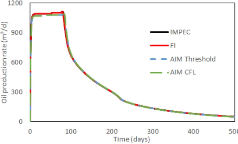
Figure 11 – Oil production rates for Case study 1 (QOFS-3comp). . . 67

Figure 12 – Gas production rates for Case study 1 (QOFS-3comp). . . 67

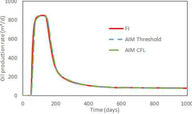
Figure 13 – Oil production rates for Case study 2 (QOFS-6comp). . . 69

Figure 14 – Gas production rates for Case study 2 (QOFS-6comp). . . 69

Figure 15 – Oil production rates for various CFL values (QOFS-3comp). . . 71

Figure 16 – Gas production rates for various CFL values (QOFS-3comp). . . 71

Figure 17 – Oil production rates for various CFL values (QOFS-6comp). . . 72

Figure 18 – Gas production rates for various CFL values (QOFS-6comp). . . 72

Figure 19 – Two-dimensional meshes: (a) 7,449 nodes with triangular elements and (b) 7,942 nodes with mixed elements. . . 73

Figure 20 – Oil production rates comparison for the 7,021 nodes quadrilateral mesh (QOFS-3comp case). . . 74

Figure 21 – Gas production rates comparison for the 7,021 nodes quadrilateral mesh (QOFS-3comp case). . . 74

Figure 22 – Gas saturation profile at 100 days for Case 1. . . 75

Figure 23 – Oil production rates comparison for the 7,449 nodes triangular mesh (QOFS-3comp case). . . 75

3comp case). . . 76 Figure 26 – Gas production rates comparison for the 7,942 nodes mixed mesh

(QOFS-3comp case). . . 76 Figure 27 – Oil production rates comparison for the 7,021 nodes quadrilateral mesh

(QOFS-6comp case). . . 77 Figure 28 – Gas production rates comparison for the 7,021 nodes quadrilateral mesh

(QOFS-6comp case). . . 77 Figure 29 – Gas saturation profile at 1300 days for Case 2. . . 78 Figure 30 – Oil production rates comparison for the 7,449 nodes triangular mesh

(QOFS-6comp). . . 79 Figure 31 – Gas production rates comparison for the 7,449 nodes triangular mesh

(QOFS-6comp case). . . 79 Figure 32 – Oil production rates comparison for 7,942 nodes mixed mesh (QOFS-6comp). 80 Figure 33 – Gas production rates comparison for 7,942 nodes mixed mesh (QOFS-6comp). 80 Figure 34 – Three-dimensional 19,044 volumes grid composed of hexahedron elements. 81 Figure 35 – Oil production rates comparison for the 19,044 nodes hexahedron elements

mesh. . . 81 Figure 36 – Gas production rates comparison for the 19,044 nodes hexahedron elements

mesh. . . 81 Figure 37 – Gas saturation field at 150 days for the QOFS-6comp 3D case. . . 82 Figure 38 – Two-dimensional irregular reservoir grid composed of 27,271 nodes. . . 83 Figure 39 – Porosity field for two-dimensional irregular reservoir grid composed of 27,271

nodes. . . 83 Figure 40 – X and Y permeability field for two-dimensional irregular reservoir grid

composed of 27,271 nodes. . . 83 Figure 41 – Oil production rates comparison for the 27,271 nodes mixed elements mesh. 84 Figure 42 – Gas production rates comparison for the 27,271 nodes mixed elements mesh. 84 Figure 43 – Gas saturation field at 150 days for two-dimensional irregular reservoir grid

composed of 27,271 nodes. . . 85 Figure 44 – Three-dimensional 19,928 volumes grid composed of hexahedron,

Figure 46 – Gas production rates comparison for the 19,928 nodes mesh. . . 87 Figure 47 – Gas saturation field at 700 days for the 19,928 volumes mesh. . . 88 Figure 48 – Grid element formed by the (1), (2), (3) and (4) vertices. . . 97 Figure 49 – Threshold AIM Oil production rates comparison for the 7,021 nodes

quadri-lateral elements mesh (QOFS-3comp case). . . 99 Figure 50 – Threshold AIM Gas production rates comparison for the 7,021 nodes

quadri-lateral elements mesh (QOFS-3comp case). . . 99 Figure 51 – Threshold AIM Oil production rates comparison for the 7,449 nodes

triangu-lar elements mesh (QOFS-3comp case). . . 100 Figure 52 – Threshold AIM Gas production rates comparison for the 7,449 nodes

triangu-lar elements mesh (QOFS-3comp case). . . 100 Figure 53 – Threshold AIM Oil production rates comparison for the 7,942 nodes mixed

elements mesh (QOFS-3comp case). . . 101 Figure 54 – Threshold AIM Gas production rates comparison for the 7,942 nodes mixed

elements mesh (QOFS-3comp case). . . 101 Figure 55 – Threshold AIM Oil production rates comparison for the 7,021 nodes

quadri-lateral mesh (QOFS-6comp case). . . 102 Figure 56 – Threshold AIM Gas production rates comparison for the 7,021 nodes

quadri-lateral mesh (QOFS-6comp case). . . 103 Figure 57 – Threshold AIM Oil production rates comparison for the 7,449 nodes

triangu-lar elements mesh (QOFS-6comp case). . . 103 Figure 58 – Threshold AIM Gas production rates comparison for the 7,449 nodes

triangu-lar elements mesh (QOFS-6comp case). . . 104 Figure 59 – Threshold AIM Oil production rates comparison for the 7,942 nodes mixed

elements mesh (QOFS-6comp case). . . 105 Figure 60 – Threshold AIM Gas production rates comparison for the 7,942 nodes mixed

Table 1 – Reservoir data for case QOFS-3comp. . . 65

Table 2 – Fluid composition data for case QOFS-3comp. . . 65

Table 3 – Component data for case QOFS-3comp. . . 65

Table 4 – Operational conditions for case QOFS-3comp. . . 66

Table 5 – Binary interaction coefficient data for case QOFS-3comp. . . 66

Table 6 – Relative permeability data for case QOFS-3comp. . . 66

Table 7 – Simulation data for case QOFS-3comp. . . 66

Table 8 – Reservoir data for case QOFS-6comp. . . 68

Table 9 – Fluid composition data for case QOFS-6comp. . . 68

Table 10 – Component data for case QOFS-6comp. . . 68

Table 11 – Operational conditions for case QOFS-6comp. . . 68

Table 12 – Binary interaction coefficient data for case QOFS-6comp. . . 69

Table 13 – Relative permeability data for case QOFS-6comp. . . 69

Table 14 – Simulation data for case QOFS-6comp. . . 70

Table 15 – Simulation data for various CFL values (QOFS-3comp). . . 71

Table 16 – Simulation data for various CFL values (QOFS-6comp). . . 72

Table 17 – Simulation data comparison for 7,021 nodes quadrilateral mesh (QOFS-3comp). 74 Table 18 – Simulation data comparison for 7,449 nodes triangular mesh (QOFS-3comp). 76 Table 19 – Simulation data comparison for 7,942 nodes mixed mesh (QOFS-3comp). . . 77

Table 20 – Simulation data comparison for 7,021 nodes quadrilateral mesh (QOFS-6comp). 78 Table 21 – Simulation data comparison for 7,449 nodes triangular mesh (QOFS-6comp). 78 Table 22 – Simulation data comparison for 7,942 nodes mixed mesh (QOFS-6comp). . . 79

Table 23 – Simulation data comparison for 19,044 nodes hexahedron elements mesh. . . 82

Table 24 – Molar balance error data for 19,044 nodes hexahedron elements mesh. . . 82

Table 25 – Simulation data comparison for 27,271 nodes mixed elements mesh. . . 84

Table 26 – Molar balance error data for 27,271 nodes mixed elements mesh. . . 85

Table 27 – Permeability tensor for 3D irregular reservoir-6comp case. . . 86

Table 28 – Operational conditions for the Irregular grid-6comp case. . . 86

Table 29 – Simulation data comparison for 19,928 nodes mesh. . . 87

ments mesh (QOFS-3comp). . . 101 Table 32 – Threshold AIM Simulation data comparison for 7,942 nodes mixed elements

mesh (QOFS-3comp). . . 102 Table 33 – Threshold AIM Simulation data comparison for 7,021 nodes quadrilateral

mesh (QOFS-6comp). . . 103 Table 34 – Threshold AIM Simulation data comparison for 7,449 nodes triangular

ele-ments mesh (QOFS-6comp). . . 104 Table 35 – Threshold AIM Simulation data comparison for 7,942 nodes mixed elements

a Equation of state parameter

A Area

b Equation of state parameter

Cf Rock compressibility

D Depth

fi j Fugacity

F Gibbs phase rule degrees of freedom

Fi CFL function

g Gravity

GT Total Gibbs free energy

kr j Phase relative permeability ⇒

K Formation absolute permeability tensor ⇒

Kj Effective permeability tensor

Lj Phase mole fraction

MWi Molar mass

np Number of fluid phases

nc Number of hydrocarbon components

Ni Number of moles ˜

Ni Shape function

P Pressure

Pc Capillary pressure

qi Component molar flow rate

Qj Phase volumetric flow rate

R Universal gas constant

Sj Phase saturation

~uj Phase velocity

Vp Pore volume

Vt Total fluid volume

W I Well index

xi j Component phase molar fraction

Z Compressibility factor

ρj Phase mass density

ξj Phase molar density

µj Phase viscosity

µ_{i j} Chemical potential

λj Phase mobility

φ Porosity

Φ_j Phase hydraulic potential

ν Molar volume

1 INTRODUCTION . . . 17

1.1 Reservoir Simulation . . . 17

1.2 Research Objectives . . . 18

1.3 Chapters Overview . . . 18

2 LITERATURE REVIEW . . . 20

2.1 Numerical Formulations . . . 20

2.2 Adaptive Implicit Methods. . . 26

2.3 Griding . . . 29

3 PHYSICAL MODEL . . . 33

3.1 Material Balance Equations . . . 34

3.2 Constraint Equations. . . 35

3.3 Thermodynamic Equations . . . 37

3.3.1 Phase Equilibrium . . . 37

3.3.2 Phase Behavior . . . 38

3.4 Physical Properties . . . 40

3.4.1 Molar and Mass Densities . . . 40

3.4.2 Saturation . . . 40

3.4.3 Relative Permeability . . . 41

3.4.4 Capillary Pressure . . . 42

3.4.5 Viscosity . . . 42

3.5 Source Term. . . 44

4 NUMERICAL MODEL . . . 46

4.1 EbFVM Approach . . . 46

4.2 Discretized Equations . . . 51

4.3 Interpolation Function . . . 54

5 THE ADAPTIVE IMPLICIT METHOD . . . 55

5.1 Jacobian Evaluation . . . 56

5.2 Switching Criteria . . . 59

5.2.1 Threshold Criterion . . . 60

5.2.2 CFL-based Criterion . . . 60

6.1.1 Case study 1 . . . 64

6.1.2 Case study 2 . . . 67

6.2 Stable CFL Limit . . . 70

6.2.1 Case study 1 . . . 70

6.2.2 Case study 2 . . . 70

6.3 Comparison Between AIM, IMPEC and FI . . . 72

6.3.1 QOFS-3comp 2D . . . 73

6.3.2 QOFS-6comp 2D . . . 76

6.3.3 QOFS-6comp 3D . . . 80

6.3.4 2D Irregular reservoir-6comp . . . 82

6.3.5 3D Irregular reservoir-6comp . . . 85

7 CONCLUSIONS . . . 89

7.1 Future work . . . 90

BIBLIOGRAPHY . . . 91

APÊNDICES . . . 97

APPENDIX A – Implicitness Level Influence on Jacobian Matrix Equations 97 APPENDIX B – Threshold Optimization Procedure . . . 99

B.1 QOFS-3comp 2D . . . 99

B.2 QOFS-6comp 2D . . . 102

APPENDIX C – Newton-Raphson Convergence Criteria . . . 106

1 INTRODUCTION

This introductory chapter aims to present a general view of reservoir engineering and the related numerical simulation. Afterwards, the main objectives and importance of the work are presented, and a brief summary of the chapters is described.

1.1 Reservoir Simulation

The importance of the oil and gas industry is a commonly known fact. Its final products are applied in large scale on an enormous variety of fields, which explains the size of this market. For instance, in 2016, the Brazilian production went up to 2.144 million barrels per day (ECONOMIA, 2017). In the US, an average of 12.704 millions barrels per day were produced in 2015 (STATISTA, 2017). An expected consequence of theses number is the impact on global markets. For decades, the economy has been profoundly affected by the result of political events on oil prices.

Given this scenario, it is no surprise that oil production has attracted the attention of companies and research groups in a continuous effort to improve efficiency and reduce risks. Evaluating the entire petroleum chain, extracting oil is likely the most uncertainty prone step. The advent of computational simulators produced a huge impact on this field, since these tools enabled a much faster increase on effectiveness in a few decades than observed before. Reservoir simulation has become a key instrument for companies evaluating new and old prospects, as well as academic researches studying new production processes.

1.2 Research Objectives

The first goal of this work is to implement and verify the advantages of an Adaptive Implicit Method (AIM) when compared with other methods. The new model is born from the combination of the ACS et al. (1985) Implicit Pressure, Explicit Composition and the FERNANDES (2014) formulations. These are also the techniques against which the comparison is performed.

Achieving this objective requires the evaluation of production curves accuracy and performance in terms of CPU time. Several two and three-dimensional case studies, mainly gas flooding problems, are applied in multiple reservoir geometries. We should note the different fluids produce very distinct problems concerning the phase behavior, giving a chance to see how the scheme performs.

Another major aspect considered is the role of switching criterion for the AIM. A weak shifting algorithm can effectively undermine any performance improvement and produce instabilities. Therefore, a complementary objective of the present study is to implement two already reportedly used criteria. All comparisons are done for both approaches in order to understand their behavior in various situations.

Finally, we aim at combining the AIM with Element-based Finite Volume Method unstructured grids. This represents the chief scientific contribution of the research, since there are not many studies concerning the association of these methodologies. All these points combined can produce a new, faster and reliable formulation.

1.3 Chapters Overview

Chapter 2 provides an analysis on the state of art in reservoir simulation. The focus lies first on numerical formulations, the different approaches and increasing complexity. In sequence, an evaluation of the adaptive methods is presented. Finally, griding techniques are reviewed aiming specifically unstructured meshes.

Following, Chapter 3 shows the mathematical model behind the implemented for-mulation. The chapter sections investigate the material balances (flow equations), constraint relations and phase behavior description for a compositional scheme.

THOMAS; THURNAL (1982) and COATS (2001) switching criteria.

2 LITERATURE REVIEW

This chapter is dedicated to review the main aspects discussed in this work as an effort to verify contributions to the state of art on reservoir simulation. Three sections explore each specific matter: the development of numerical formulations; the advent and evolution of the Adaptive Implicit approach; and griding techniques, with special focus on unstructured meshes.

2.1 Numerical Formulations

Petroleum reservoir simulation is a relatively recent area of study. The theoretical basis behind multiphase flow in porous media was known for quite some time. However, the model’s complexity, composed of several equations and unknowns, made its application prohibitive. Before the second half of the 20th century, most models were extremely simple and based on analytic solutions for overall material balances or one-dimensional problems (COATS, 1982). These were far from reproducing actual field applications and limited to very specific analysis. For instance, one of the first applied techniques was proposed by Buckley e Leverett (1942). Their analytical model described incompressible and immiscible flow up to two phases. The advent of computers and their rapid advancement allowed for the development of more sophisticated numerical methods which led to a surge on the amount of works published in the matter (COATS, 1982). These simulators, developed around the 1960’s, also presented some limitations. Most methods focused on two-phase and three-phase black oil problems, as well as recovery methods associated to depletion or pressure maintenance. Most field applications were actually well described by theses models, posing no serious issues.

The scenario dramatically changed in the next decade. The 1973 Oil Crisis was the first of a series of politically motivated embargoes that caused a fast rise of oil prices on the international market (GUARDIAN, 2011), which in turn allowed for the widespread implementation of enhanced oil recovery (EOR) processes. More complex simulators were developed in order to describe phenomenons such as miscible flow, chemical injection and CO2 injection, as well as handle more elaborate equilibrium calculations. Kazemiet al.(1978) was one of the first to propose a compositional formulation for three-dimensional reservoir with up to three fluid phases, while still evaluating phase equilibrium calculations through correlations. As a consequence, phase related properties calculation generated relevant convergence issues.

into their simulator , and showed how it improves the convergence rates. From this point on, most models proposed in the literature also will lay hand of advantages of using EOS. However, before we proceed further, there should be a deeper investigation on the concept of formulation in order to better differentiate the studies mentioned in this work. Describing flow in porous medium requires the evaluation of several variables, specially if we are dealing with multiphase and multicomponent fluids. Computing all these unknowns in an iterative procedure leads to a huge computational effort, therefore many algorithms, or formulations, have been proposed to optimize performance and guarantee stability. It is important to note not all properties must be computed in order to define a system, as expressed by the Gibb’s phase rule:

F =n+2₋np (2.1)

The above expression calculates the minimum amount of intensive properties re-quired to describe a thermodynamic state (F), also called degrees of freedom, as a function of both the number of phases (np) and components (n) in equilibrium. Once these unknowns are evaluated, all remaining properties are computed afterwards. It is important to highlight applying this expression assumes the local equilibrium condition, meaning every point in the reservoir must be in phase equilibrium. Additionally, adjustments are required for the reservoir production specific case. First, the methodology developed in this work, in accordance with several studies in the literature, is isothermal, meaning one less intensive property to be determined. Following, another usual procedure applied here is to remove water from the flash calculations. This requires two modifications on Eq. (2.1): replacingnfor the number of hydrocarbon components (nc), and

npfornp−1. Finally, the evaluation of phase flow demands the calculation of phase saturations, adding anothernp−1 degrees of freedom, since the saturation constraint can be used to compute the remaining saturation.

np

∑

Sj=1 (2.2)

All theses changes implemented make Eq. (2.1) assume the form:

F =nc+1 (2.3)

remainder of properties, called secondary variables, are all computed as a functions of them. Additionally, the extensive state is defined if we include a single more degree of freedom, like, for instance, a hydrocarbon component amount of moles. The definition of primary and secondary variables is relevant mainly because all reservoir simulations models apply them into their scope. For instance, Fussel e Fussel (1979) applies a dynamic primary variables selection. Apart from pressure, the remaining state defining unknowns are chose according to the predominant phase in each grid block. Should more gas phase moles be present in a given control volume, the amount of oil phase moles per pore volume and nc−1 oil phase compositions are selected. The procedure is analogous for oil phase predominant volumes. From these variables, only the pressure is treated implicit, yielding an Implicit Pressure/ Explicit Composition (IMPEC) model. The first Fully Implicit model for compositional simulation was proposed by Coats (1980). The Redlich e Kwong (1949) EOS is used to describe phase behavior. Additionally, the author chooses to account for capillary, gravity and viscous forces. Only physical dispersion is neglected. As the name suggests, this approach means to treat all primary variables implicit. Initially, each Jacobian matrix entry has a 2nc+4 size, accounting for oil and gas phases molar fractions, all saturations and pressure. A Gaussian elimination decouples the secondary unknowns from the linear system, yieldingnc+1 sized entries. We should note the remaining primary variables are dependent on the amount of phases present in each grid block. For the case the two hydrocarbon phases exist, the gas phase pressure, both saturations andnc−2 gas compositions are chosen. If only the gas phase is encountered, the pressure, saturation andnc−1 compositions for the gas phase are the primary unknowns. The choice is analogous for volumes containing only the oil phase. The author reports stable runs even for thermodynamic conditions close to the critical point, while noting significant numerical dispersion. The FI method, as largely reported in the literature, served as the counterpoint for the IMPES, since it guarantees great stability at the cost of larger Jacobian matrix. This concept is further developed later on this chapter.

not able to attain quadratic convergence. Young e Stephenson (1983) also proposed changes to IMPEC model. The authors modified the Jacobian matrix structure from Fussel e Fussel (1979), reordering equations in an effort to improve efficiency and facilitate the insertion of new fluid properties correlations. As for the primary variables, there is no dependence on the number of existing phases. The chosen parameters are pressure, gas phase amount of moles per pore volume, andnc−1 gas phase compositions.

A new IMPEC approach was shown by Acs et al.(1985). A volume constraint is the basis for the pressure equation. This feature itself is not innovative. Both Kazemi et al. (1978) and Nghiemet al.(1981) used this notion. The difference, however, lies in the procedure. Starting from the assumption the total fluid volume must equal the pore volume, both terms are expanded by a Taylor series truncated in the first order term. The equation generated from this development is unique for it is completely decoupled from phase behavior calculations and its discretized version is linear. This produces an important consequence. Since no non-linearities exist, there is no need for an Newton iterative procedure. Another significant change is on the primary variables. The authors argue phase saturations, as volumetric ratios, are not usual thermodynamic parameters. Instead, pressure and the nc component masses are selected. It should be noted, however, the method presents two rather undesirable features. First, obtaining the pressure equation requires computing total fluid volume derivatives, a complex task not describe in Acs et al. (1985). Following, the truncation on the first order term demands a volumetric error term to be placed into the equation. This addition, however described as a means to maintain the volumetric error stable and allow large time steps, not always produces the desired effect (WONGet al., 1990).

Chienet al.(1985) designed a variation from the Coats (1980) model. The parameters are decoupled from the linear system in the same manner. However, the authors opted for a different set of primary variables. Pressure, nc(np−1) phase equilibrium ratios, water and

nc−1 hydrocarbon components overall molar fraction are selected. This group yieldsnc(np−1) extra variables than required by Eq. (2.3). The pivotal unknowns, as named by the authors, are removed from the matrix. Finally, only pressure and the overall molar fractions are solved implicit.

Following thenp−1 phase saturations are also implicitly computed. This requires an evaluation of phase velocities between the two steps, meaning morenpimplicit parameters. Goods results are reported while highlighting the method presents inherit inconsistencies generated from the phase velocities evaluation and the molar fractions treatment. The author does not discusses this matter beyond mention, and notes no relevant errors were observed.

Later, Quandalle e Savary (1989) addressed these matters. They verified two main sources for the already mentioned inconsistencies. One of them is related to the relative perme-abilities and capillary pressures. When solving the pressure linear system, these properties are treated explicit. Nevertheless, computing saturations demands an implicit evaluation of the same parameters. The second issue is observed by the factnc+1 flow equations are able to provide a solution fornc+2 unknowns. As a consequence, the gas phase saturation is evaluated in two different ways: a secondary variable obtained as a result of the flash calculations and, at the same time, an input parameter for calculating the implicit relative permeabilities and capillary pressures. The authors define extranc−2 compositional parameters for the flow equations. A set of primary variables is built by these new unknowns, the oil phase pressure, gas and water phases saturations. Further, the relative permeabilities and capillary pressures are submitted to an implicit approximation in the event of computing the interblock flow terms in the pressure equation.

leads to smaller maximum time steps, also effecting run CPU times. The authors also found many similarities between the two sets of formulations, such as in the Jacobian matrix. This is also verified in the computed derivatives. While VB methods obtain it through direct analytic calculations, the same values appear as a consequence of the Gaussian elimination in NR techniques.

Watts et al. (1991) proposed a Fully Implicit variation of Acs et al. (1985) for thermal simulation. The authors argue this approach was necessary to handle thermal recovery processes, once the level of implicitness of Acset al.(1985) and Watts (1986) was not enough to handle the high flow rates near wells and the strong coupling between energy and flow equations. Comparison with commercial packages revealed competitive results. Also on modified models, Branco e Rodriguez (1996) presented an approach with a implicitness degree between FI formulations and Watts (1986). Within an iterative step, compositions are fixed and all unknowns but pressure andnp−1 phase saturations are decoupled from the Jacobian matrix, yieldingnpxnp sized entries. Only after the implicit parameters are computed, the evaluation of compositions and remaining properties is performed.

Wanget al.(1997) aimed reducing the non-linearities in the fugacity equation and, therefore, improve convergence. This was done by choosing pressure,ncamount of hydrocarbon component moles and thencequilibrium ratio logarithms on their FI formulation. It should be noted, however, theln(K)parameters are removed from the linear system through factorization and solved only afterwards.

2.2 Adaptive Implicit Methods

For several years, most simulators applied implicit pressure, explicit saturation (IMPES) models or its variations, mainly because those were the only techniques capable of handling field scale problems due to limited computational resources. Fully Implicit models were limited to a few theoretical case studies. The memory and computational effort required for this approach made the application on more complex problems prohibitive. At the same time, explicit techniques imposed severe restrictions to time step size, specially for some specific regions of the reservoir like well surroundings, as in coning studies (COLLINSet al., 1992)), and saturation fronts.

Thomas e Thurnal (1983) and Thomas e Thurnal (1983)) set up the first black oil Adaptive Implicit Method, which will also be referred as TT from now on, by acknowledging there is no need to treat the entire simulation domain FI. At any given time step during a run, some regions of the reservoir present potential sources of instability IMPEC methods are not able to handle. The authors argue only these areas need the maximum level of implicitness. This way only a certain amount of variables really need to be calculated into the linear system, reducing the computational effort required and allowing large time steps. Each primary unknown was computed implicit if its total variation over the previous time step exceeded a previously defined threshold. This stability test is based on Peaceman (1977) with some extrapolation. The authors note these property variation limit values do not hold any theoretical basis and each simulation should be submitted to preliminary trial runs in order to achieve optimal thresholds.

Another variation, the Inexact Adaptive Newton (IAN) method, was presented by Bertiger e Kelsey (1985), where the off-diagonal Jacobian matrix coefficients relating to the explicit unknowns are only removed. This yields a linear system closer to the Fully Implicit models, which, as argued by the authors, can produce more stable runs in comparison with AIM. However, this approach is non-conservative in essence, causing a new possibly source of instability. Tan (1988) addresses this issue by reintroducing the residual errors as source terms in the respective equations in the next time step, reporting successful limitation the material errors.

to implicit) are allowed until another well becomes operational and the procedures starts again. The authors reported stable runs and optimized CPU times in comparison with a FI model. Another major modification concerned the evaluation of explicit unknowns. As proposed by Thomas e Thurnal (1982), at each Newtonian iterative step, the explicit variables are updated following the primary unknowns evaluation. This new approach first obtained the Newton-Raphson iterative procedure convergence for the implicit unknowns. Only then, all explicit properties were computed. Russel (1989) compared both methodologies, noting the AIM label would better suit the latter, while TT actually provided a shortcut to the FI solution. We should emphasize there is not an overall consensus about this matter.

Later, alternatives to the threshold switching criterion were the subject of many works. Forsyth (1989) argued the original approach aimed to bound the model solution, which does not necessarily guarantees stability. The author then proposed another threshold to preserve monotonicity, which in term would lead to stable runs. Funget al.(1989) developed an entirely different numerical test for black oil simulations aiming to improve the AIM stability. The principle was to predict whether numerical errors would increase in the next time step for each grid volume, and then set implicit all primary variables in these blocks. The backward switching, from implicit to explicit, followed an analogous procedure, and would leave only pressure inside the Jacobian matrix, as in an IMPEC model. Similar results to the original threshold criterion were found while avoiding the trial and error procedure. This procedure was, however, too cumbersome to be applied in the entire grid. Therefore, only the blocks in the IMPES/FI interface were tested every few time steps. At the same time, Grabenstetteret al.(1991) noted the numerical criterion was develop to identify whether the entire domain was unstable. In turn, Fung et al.(1989) simplify the method for single volumes stability check without profound discussion on its merit.

relevant instability. It should be noted both Russel (1989) and Grabenstetteret al.(1991) methods are advantageous in face of Funget al.(1989) approach, for most required derivatives are already computed on a simulator, greatly reducing the computational effort. The Grabenstetter et al. (1991) formulation was studied by Collins et al. (1992), outperforming both IMPEC and FI formulations. We should note Collins et al.(1992) decouples the flash calculations from the primary equations, similar to Forsyth e Sammon (1986).

The CFL condition was also the subject of Young e Russel (1993). The authors proposed a more robust mixed switching criterion. A CFL based criterion is written in such a way to account for the influence of all downstream neighbors for any given block, and supported by a complementary threshold. This addition is rendered necessary once the CFL criterion itself does not guarantee stability in problems where strong nonlinearities occur. This set up, the authors point, allows for the CFL limit to exceed the unity. Good results are reported in comparison with Fully Implicit models. However, it is highlighted the comparative performance with IMPES does not show significant enhancements. Meanwhile, the AIM approach was also evaluated for thermal simulators by Farkas e Valko (1994). The authors observed that coupling mass and energy constraint equations could impose even stricter time step size limitations. Hence, a direct IMPES formulation, derived from the Acset al.(1985) method, is proposed as the basis for a adaptive technique.

main difference lies on an exclusive CFL function for temperature, which in turn means three implicitness degrees are possible.

The Coats (2001) stability test is used in Cao e Aziz (2002) for their new technique, the IMPSAT based adaptive implicit model (IMPSAT-AIM). The authors argue the IMPSAT can outperform both IMPEC and FI, given its intermediate level of implicitness. Hence, the new adaptive approach admits a third evaluation for any given volume, yielding a combination of FI, IMPES and IMPSAT formulations. The reported results indicate the new model can consistently outperform the traditional AIM.

2.3 Griding

In order to implement all numerical formulations discussed in the previous sections it is necessary the spacial discretization of the model equations. This procedure, which allows problems to be evaluated at a discreet number of points, needs to be performed in a way to reduce simulation errors. We should also note all methods can respond well to different discretization, once their derivations are relatively grid independent. Still, for many decades all reservoir numerical calculations were based on orthogonal Cartesian grids. Spatial derivatives are usually described on the orthogonal system, which in turn makes it only "natural" to follow the same approach in a simulator (WADSLEY, 1980). However, as observed by Funget al.(1992), the application of Finite-Volume Methods (FVM) in conjunction with Cartesian grids produces a series of issues when attempting to describe complex geometries and discontinuities, which are almost unanimously present in real field simulations. Furthermore, Pedrosa e Aziz (1986) noted this type of mesh cannot satisfactorily represent near well flow.

The first alternative largely applied on reservoir simulators were the Boundary Fitted (BF) meshes, also known as Corner Point (CP) grids. Their assessment is actually similar to the Cartesian discretization. These are still structured orthogonal meshes. However, the BF approach dictates the grid has to fit the domain boundaries, hence its name. Their application on reservoir engineering dates the work of Sheldon e Dougherty (1961) on front-tracking simulation for open pattern displacements. Hirasaki e O’Dell (1970) applied this method for simulations on reservoir with changing dip and thickness, and stated the new approach presents a much more accurate portrait of the geometry, leading to lower numerical errors. Similar results are reported by Wadsley (1980).

before also occurring on relevant numerical errors, causing accuracy issues. Leventhal et al. (1985) was able to avoid this problem adjusting the grid lines tangent to match the streamlines on a single phase flow solution. A Non-Orthogonal BF (NOBF) technique, a presented by Chu (1971), proved to better address such cases. Nevertheless, this approach would only gain notoriety after the study conducted by Thompsonet al.(1974). Maliska e Raithby (1984) applied the NOBF to fluid problems on varying cross-sectional ducts for two and three-dimensional grids. The authors report the mesh layout greatly influences the linear system shape, defining the number of points on the pressure equation. Later, the same approach was applied by Cunhaet

al.(1994) for two-phase (water + oil) black oil simulations with 2D meshes. The results show NOBF can mitigate grid orientation effects. Maliskaet al.(1994) presented similar results for black oil three-dimensional problems. Later, Maliska et al.(1997) combined the NOBF with a black oil Fully Implicit approach using pressure and mass fractions as primary unknowns. A well model is also proposed to address non-orthogonality. Edwards (1998) adopted another approach, by retaining the same linear system bandwidth as in Cartesian grid discretization, and inserting the cross-flux terms into the residual term. The author argues the method provides more accurate results in comparison with orthogonal alternatives, while better handling full tensors. Marcondeset al.(2005) expanded Maliskaet al.(1997) for FI compositional simulation. Good agreement was found for three-dimensional water flooding problems, while mesh orientation effects were not reported. The authors also evaluated the Boundary Fitted method in conjunction with parallel computing, obtaining good speedups for a relative large number of processors. Regarding cross-flow terms, Marcondeset al.(2008) showed their absence in the linear system can produce relevant discrepancies even for meshes with small distortion levels.

proposed the name Element-based Finite Volume Method (EbFVM). This nomenclature has been increasingly adopted since then. In the present work, the author will also apply the EbFVM label.

Unstructured grids in reservoir simulation first appeared on Heinemann e Brand (1988), closely followed by Heinemann et al. (1989). The presented method generates the Perpendicular Bisection (PEBI) grids. This approach requires the grid to be constructed in a way all interfaces between two neighboring control volumes must be perpendicular to the line segment composed by the center of these volumes. The consequence is only two points are taken into account when evaluating fluxes though any given interface.

Rozon (1989) was the first to apply unstructured EbFVM meshes into reservoir simulation. Its work was limited to single phase flow problems using meshes composed only of quadrilateral elements. The author compares the method with an analytic solution, reporting a good agreement. Forsyth (1990) used the EbFVM grids on local grid refinement. Consistent computational time was observed for both FI and AIM. Funget al.(1992) went further, applying the EbFVM for multiphase flow problems in meshes of triangle elements. The results show the unstructured discretization outperforms Cartesian grids while allowing for local grid refinement without occurring on numerical errors. Darwish e Moukalled (2003) investigated Total Volume Diminishing (TVD) interpolations functions, originally developed for Cartesian meshes, in conjunction with unstructured grids. An extended analysis on this matter was performed by Fernandeset al.(2003). The authors adapted the work of Darwish e Moukalled (2003) on TVD schemes, implementing the MINMOD (ROE, 1986) and Koren (KOREN, 1993) flux limiters. Other interpolation functions are applied on unstructured grids by Fernandeset al.(2003): the Mass Weighted Upwind scheme (MAW) (Massonet al.(1994); Saabas e Baliga (1994a); Saabas e Baliga (1994b)), the Hurtadoet al.(2007) modified MAW, and a Streamline based Upwind method (Swaminathan e Voller (1992a); Swaminathan e Voller (1992b)).

3 PHYSICAL MODEL

As mentioned earlier, reservoirs are porous media in which various hydrocarbon components are unevenly distributed over several fluid phases. The most usually observed phases are water, oil, gas. Modeling such systems requires the evaluation of material balances, phase behavior and constraint equations. The last two set of expressions arise from the necessity to properly describe multiple fluid phases and the mass transfer between then.

The physical model applied in this work is built on a series of assumptions listed below:

1. Isothermal system.

2. Slightly compressible porous medium. 3. No-flow reservoir boundaries.

4. Flow is described by the multiphase Darcy’s law. 5. Physical dispersion is neglected.

6. Local phase equilibrium. 7. No chemical reactions occur.

8. The mass transfer between the water and hydrocarbon phases is neglected. 9. There are a maximum of two hydrocarbon phases in equilibrium.

All of these simplification hypothesis are widely used on academic and commercial simulators. Even so, we must discuss some of the listed items. First, the implications of the two last assumptions are investigated. Both of them relate to the amount of phases in thermodynamic equilibrium. For several applications, such hypothesis would not cause any concern. However, the results for the proposed formulation are obtained using gas flooding case studies. Additionally, these problems are characterized byCO2rich injection fluids. Such conditions, combined with the right thermodynamic state, may favor mass transfer between water and hydrocarbon phases, as well as the appearance of an extra hydrocarbon phase. Also, the physical dispersion influence might not be negligible for highly miscible phases. Nevertheless, we choose to maintain these simplifications in order to avoid the additional numerical complexity which their evaluation would produce. At the same time, the applied case studies have been severely tested with various formulations, constituting effective means of validating the work.

3.1 Material Balance Equations

Compositional models imply several hydrocarbon components (or pseudo-components) which may be present in several phases. This way, the material balance equation for each of the hydrocarbon components are described as in Chang (1990). After neglecting the physical dispersion term, they are given by

∂

∂t φ

np

∑

ξjSjxi j !

+~∇_· np

∑

ξjxi j~uj !

+q˙i Vb

=0, i=1, ...,nc (3.1)

whereφ stands for the medium porosity, ξj denotes the phase molar density, Sj is the phase saturation,xi j is thei−thcomponent molar fraction in the j−thphase,~ujdenotes the phase velocity vector, qi is the i−th component source/sink term andVb is the bulk volume. This equation is also written in similar fashion for water:

∂

∂t(φ ξwSw) +~∇·(ξw~uw) + ˙ qw Vb

=0 (3.2)

where thewsubscript denotes all the above mentioned properties are evaluated for the water phase. The first term on both balance equations represents the number of component moles variation with respect to time. This can be shown defining the total amount of moles for the

i₋thhydrocarbon component, as well as for water.

Ni=Vbφ np

∑

ξjSjxi j, i=1, ...,nc (3.3)

Nw=Vbφ ξwSw (3.4)

Replacing Eqs. (3.3) and (3.4) respectively into Eqs. (3.1) and (3.2) yields the modified material balances equations after some manipulation.

1 V_b

∂Ni ∂t +~∇·

np

∑

ξjxi j~uj !

+ q˙i

V_b =0, i=1, ...,nc (3.5)

1 Vb

∂Nw

∂t +

~_{∇·(ξw~uw) +}q˙w Vb

=0 (3.6)

Equations (3.5) and (3.6) require the evaluation of~uj. From assumption (4.), the phase velocities are computed by the Darcy’s law for multiphase flow, written as

~ uj=−

1 µj

⇒

whereµj is the phase viscosity,Φjdenotes the phase hydraulic potential, and ⇒

Kjis the effective permeability tensor. The last two parameters are described by the following expressions:

Φ_j=Pj−ρjgD, j=1, ...,np (3.8)

⇒ Kj=kr j

⇒

K, j=1, ...,np (3.9)

In Eqs. (3.8) and (3.9)Pj is the phase pressure,ρjdenotes the phase mass density,g is the gravity acceleration andDstands for the depth (positive in the downward direction),kr j is the j₋thphase relative permeability with respect to the reference phase, and

⇒

K denotes the formation absolute permeability tensor. Computing the phase pressures requires the evaluation of the capillary pressure relations. From a reference phase, set as the oil in UTCOMP, the capillary pressure relations with the remaining phases are computed.

Pj=Pr+Pc jr, j=1, ...,np (3.10)

wherePc jrstands for the capillary pressure between the j−thand the reference phase. These material balances yield the firstnc+1 primary equations. Previously, it was noted the system definition in intensive terms demands one more equation. The remaining expression is presented in the next section for it derives from a physical constraint condition.

3.2 Constraint Equations

The material balances shown require some physical constraints. It is important to notice these restrictions arise from the very definitions of some properties, such as phase saturations and molar fractions, as follows:

np

∑

Sj=1 (3.11)

nc

∑

xi j =1, j=1, ...,np (3.12)

the pressure equation as described by Acset al.(1985). Its development start with Eq. (3.13) below:

Vt

P,~N

=Vp(P) (3.13)

This equation basically states the total fluid volumeVtneeds to be precisely the same as the pore volumeVp. It also assumes the left hand side of the equation to be a function of both pressure and the total amount of moles of each component~_{N= (N1, ...,Nn}

c,Nnc+1). As for the

right hand side, the pore volume is taken solely as a pressure function. Deriving both sides of the equation with respect to time, and applying the chain rule yields the following expression:

∂Vt ∂P

Ni

∂P ∂t +

nc+1

∑

"

∂Vt ∂Ni

P,Nk(k₆=i)

∂Ni ∂t

#

=∂Vp ∂P

∂P

∂t (3.14)

Before we advance further, it is convenient to develop the left hand side of Eq. (3.14) defining the partial molar volume,Vti, as described in Eq. (3.15).

Vti =

∂Vt ∂Ni

P,Nk(k6=i)

(3.15)

Another important step on obtaining the pressure equation is to specify the pore volume as a pressure function. This can be achieved definingVp:

Vp=φVb (3.16)

In Eq. (3.16), the bulk volume is, for the purposes of this work, a constant and porosity, from assumption (2.), is a function of pressure described as

φ =φ0

1+Cf P−P0

(3.17)

where Cf is the rock compressibility, and φ0 is the formation porosity at a P0 reference pressure. Inserting Eqs. (3.15), (3.16) and (3.17) into Eq. (3.14) and rearranging the terms leads to

"

φ0Cf− 1 Vb ∂Vt ∂P Ni # ∂P ∂t =

1 Vb

nc+1

∑

Vti ∂Ni

∂t

(3.18)

Finally, theNiderivatives with respect to time can be obtained from Eqs. (3.5) and (3.6) simply by rearranging the equations. Once replaced into Eq. (3.18), the final pressure equation takes the form

"

φ0Cf− 1 Vb ∂Vt ∂P Ni # ∂P ∂t +Vtw

~_{∇·(ξw~uw) +}

nc

∑

Vti np

∑

~_{∇· ξjxi j~uj}

+ nc+1

∑

Vti qi Vb

=0

Equation (3.19) completes the set of primary equations. The complete model, however, still requires phase behavior and physical properties evaluation, both of which are explored in the next sections.

3.3 Thermodynamic Equations

Handling multi-phase systems requires the evaluation of phase equilibrium and thermodynamic states in order to compute several physical properties. The next sub-sections develop how these issues are tackled in the simulator.

3.3.1 Phase Equilibrium

At a given state (fixed temperature and pressure), the phase equilibrium is achieved when the total Gibbs free energyGT, described in Eq. (3.20), reaches a minimum.

GT = np

∑

nc

∑

ni jµi j (3.20)

whereni j and µi j are respectively the amount of moles and the chemical potential of component

iin phase j. The latter can be defined as follows:

µ_{i j}=µ0_{i j}+RTln fi j fi j0

,i=1, ...,nc, j=2, ...,np (3.21)

In Eq. (3.21) the superscript 0 means properties are evaluated at a reference state, and fi j denotes thei−thcomponent fugacity in phase j. This expression is simplified setting the chemical potential at the reference state as zero and fugacity as unity.

µ_{i j}=RTlnfi j,i=1, ...,nc, j=2, ...,np (3.22)

Replacing Eq. (3.22) into Eq. (3.20) and deriving the latter with respect toni j yields the total Gibbs free energy minimization condition as presented below:

lnfi j =lnfir, i=1, ...,nc, j=2, ...,np(j6=r) (3.23)

3.3.2 Phase Behavior

Once equilibrium between the hydrocarbon fluid phases is established, phase related properties need to be computed. Even though UTCOMP models phase behavior through various equations of state, only the Peng e Robinson (1976) EOS (PREOS), as implemented by Perschke (1988), is taken into account on the course of this study.

P= RT v₋b−

a

v(v+b) +b(v₋b) (3.24)

where parametersaandbare computed for pure substance as shown below:

a=Ω_aα(RTc) 2

Pc

(3.25)

b=Ω_bRTc Pc

(3.26)

The subscript c in Eqs. (3.25) and (3.26) denotes temperature and pressure are evaluated at the critical point, andRis the universal gas constant. TheΩ_aandΩ_bparameters are constant, andα is a function of the component and temperature. All three terms are presented as follows:

Ω_a=0.45724; Ω_b=0.0778 (3.27)

α =

(

1+m

"

1₋

T Tc

0.5#)2

(3.28)

wheremis computed as

m=     

0.37464+1.54226ω₋0.26992ω2, f or ω _≤0.49

0.379642+1.48503ω₋0.164423ω2+0.016666ω3, f or ω>0.49

(3.29)

In Eq. (3.29),ω denotes the acentric factor.

Equation (3.24) describes a simple one-component, two-phase system. For multi-phase/multicomponent problems, the PREOS assumes the following form:

P= RT vj−bj−

aj vj vj+bj

+bj vj−bj

Theaandbparameters are now phase related and obtained applying the mixing rule, yielding the results below:

aj= nc

∑

nc

∑

xi jxk jaik, j=2, ...,np (3.31)

bj= nc

∑

xi jbi, j=2, ...,np (3.32)

whereaikis computed as

aik= (1−κik) (aiak)0.5 (3.33)

Equation (3.33) basically allows for the binary iteration coefficientsκik influence to be accounted for on the phase behavior. The PREOS can also be described in terms of compressibility factorZ. This way, Eq. (3.30) admits the following form:

Z3_j− 1₋Bj

Z2_j+ Aj−3B2j−2Bj

Zj− AjBj−B2j−B3j

=0 (3.34)

where the parametersAjandBj are calculated as

Aj= ajP

(RT)2 (3.35)

Bj= bjP

RT (3.36)

It is important to note all above mentioned equations are solved regardingPas the oil phase pressure. Additionally, the solution of Eq. (3.34) can produce more than one real compressibility factor value. In this case, the realZj value providing the lower Gibbs free energy is chosen for each phase.

3.4 Physical Properties

In this section we present the equations applied to the fluid properties evaluation. These parameters are mainly modeled through EOS or correlations. Listed below are models for molar and mass densities, phase saturation, relative permeability, capillary pressure and viscosity.

3.4.1 Molar and Mass Densities

For the hydrocarbon phases, molar density is computed from the EOS compressibility factor:

ξj= P ZjRT

, j=2, ...,np (3.37)

The water phase is assumed slightly compressible, therefore a simple pressure function as follows:

ξw=ξw0

1+Cw P−P0

(3.38)

where ξ_w0 is the water molar density at the P0 reference pressure, and Cw is the water com-pressibility. As for the mass densities, the expression for hydrocarbon phases goes as below.

ρj=ξj nc

∑

xi jMWi (3.39)

In Eq. (3.39),MWiis thei−thcomponent molar mass. Analogously, the water mass density is computed as

ρw=ξwMWw (3.40)

3.4.2 Saturation

For hydrocarbon and water phases the saturations are respectively given by:

Sj= (1−Sw)

Lj/ξj ∑n_mp₌₂Lm/ξm

, j=2, ...,np−1 (3.41)

Sw= Nwνw

Vp

(3.42)

3.4.3 Relative Permeability

The UTCOMP has various relative permeability models implemented. For this work, only the modified Stone II approach (STONE, 1973) is taken into account. For a two-phase flow, the expressions are shown below:

krw=k0rw

Sw−Swr 1₋Swr−Sor

ew

(3.43)

kro=k0ro

So−Sor 1₋Swr−Sor

eo

(3.44)

wherekrw is the end-point permeability, Sr denotes the residual saturation and e is a model parameter.

A three-phase system version the model takes the form:

krw=k0rw

Sw−Swr 1₋Swr−Sorw

ew

(3.45)

krg=k0rg

Sg−Sgr 1₋Sgr−Swr−Sorg

eg

(3.46)

kro=k0row

krow k_row0 +krw

krog k0_row+krg

−(krw+krg)

(3.47)

wherek0_row denotes the end-point relative permeability for oil in water, Sorw and Sorg are the residual oil saturations in water and gas, respectively. Additionally, the relative permeabilities of oil in water and gas are described as follows:

krow=k0row ₁

−Sw−Sorw 1₋Swr−Sorw

eow

(3.48)

krog=krog0 ₁

−Sg−Swr−Sorg 1₋Swr−Sgr−Sorg

eog

(3.49)

The terms on Eqs. (3.48) and (3.49) are analogous to the ones previously described. Lastly, on a four-phase flow bothkrwandkrgare computed as in Eqs. (3.45) and (3.46). For the oil and second hydrocarbon liquid (l) phases, the following expressions apply:

kro=k0row So So+Sl

krow k0_row+krw

krog k0_row+krg

−(krw+krg)

(3.50)

k_rl =k0_row Sl So+Sl

krow k0_row+krw

krog k_row0 +krg

−(krw+krg)

3.4.4 Capillary Pressure

Leverett (1941) describes the capillary pressures as a function of interfacial tension, permeability, porosity and saturations. For the three-phase flow problem, the model assumes the form:

Pcwo=−Cpcσwo s

φ ky

1₋Sw

Epc _(3.52)

Pcog=−Cpcσog s

φ ky

Sw So+Sg

Epc

(3.53)

whereCpcandEpcare parameters evaluated through experimental data matching, andσ values denote the interfacial tension of the water and gas phases with respect to the oil phase. Addition-ally, theSparameters are the normalized phase saturations. For the purposes of this work, these properties are computed following the relative permeability Corey model (COREY, 1986), also implemented in UTCOMP. Their expressions follow:

Sw=

Sw−Swr 1₋Swr−Sorw−Sgr

(3.54)

So=

So−Sor 1₋Swr−Sorw−Sgr

(3.55)

Sg=

Sg−Sgr 1₋Swr−Sorw−Sgr

(3.56)

Finally, the interfacial tension between water and the hydrocarbon phases is constant and should be provided as part of the user input. On the other side, for the interfaces between two hydrocarbon phases, theσi j is calculated by the Macleod-Sugden correlation, Macleod (1923) and Sugden (1924), as a function of molar fractions, phase mole densities and the component parachor(ψk).

σ_{i j}0.25=0.016018 nc

∑

ψk ξixki−ξjxk j

, i=2, ...,np, j=2, ...,np (3.57)

3.4.5 Viscosity

is applied on this work. We begin the procedure evaluating the low-pressure, pure-component viscosity according to the Stiel e Thodos (1961) correlation.

˜ µi=

3.4x10−4_T0.94 r,i ζi

f or Tr,i≤0.15, i=1, ...,nc (3.58)

or

˜ µi=

1.776x10−4_(4.58T

r,i−1.67)5/8 ζi

, f or Tr,i>0.15, i=1, ...,nc (3.59)

whereTr,idenotes the reduced temperature andζiis a parameter computed as

ζi=

5.44T_c1_,i/6

MW1_i/2Pc2/3

, i=1, ...,nc (3.60)

The subsequent step is to apply the ˜µi in computing the low-pressure mixture viscosity as proposed by Herning e Zipperer (1936).

µ∗_j = nc

∑

xi jµ˜i√MWi/ nc

∑

xi j√MWi, j=1, ...,np (3.61)

Following, the phase viscosities are evaluated using the (Jossi) correlation:

µj=µ∗j+2.5x10−4 ξjr

ηj

f or ξjr≤0.18, j=1, ...,np (3.62)

or

µj=

µ∗_j+χ4_{j −}1 104ηj

f or ξjr>0.18, j=1, ...,np (3.63)

whereξjr is the reduced phase molar density,ηj andχj are equation parameters. These three terms are calculated as follows:

ξjr =ξj nc

∑

xi jνc,i (3.64)

ηj=5.44 nc

∑

xi jTc,i !1/6

/



 nc

∑

xi jWi

!1/2 _n c

∑

xi jPc,i !2/3

, j=1, ...,np (3.65)

3.5 Source Term

The well fluxes described in Eqs. (3.5) and (3.6) require a deeper evaluation. In this work, the Well Index (W I) approach is applied. Although several models are implemented, we only take advantage of the Peaceman (1978) and Peaceman (1983) method forW I calculation, adapting it to EbFVM meshes as reported by Funget al.(1992). Additionally, from the supported operation conditions in UTCOMP, the constant surface volumetric rate for injection wells and the constant bottom hole pressure (BHP) for both injection and producer wells are taken into account. We now discuss the source term form for each one of these conditions. Before, however, it is important to properly define the Well Index.

W Ij= ˙ qj Pw−Pj

, j=1, ...,np (3.67)

wherePwdenotes the well pressure at the point of evaluation. The Peaceman (1978) model, for vertical wells, computes the well index as below:

W Ij= p

kxky∆zλr j 25.14872lnr₀

rw

, j=1, ...,np (3.68)

In Eq. (3.68), ther0denotes the equivalent well radius, evaluate as follows:

r₀=0.28

_k

y kx

1₂

∆x2+kx ky 1₂ ∆y2 12 _k y kx 1₄

+kx ky

1₄

(3.69)

Concerning the operational conditions, for a constant surface volume injection regime the component mole flow rates are calculated at surface conditions. These rates must then be distributed among the well segments, as described below:

˙ qk,s=

"

W Is np

∑

λj,s/ ns

∑

W Il np

∑

λj,l !#

˙

qk,T, s=1, ...,ns, k=1, ...,np (3.70)

where the subscriptsdenotes the evaluation at each segment,nsis the total number of segments and ˙q_k,T the total mole flux for well. At the same time, we are able to compute the phase volumetric flow rates ˙Qj,sas follows:

˙

Qj,s=λj,sW Is Pj,s−Pw,s

Still treating injection wells, the constant BHP condition leads to the following expressions for the hydrocarbon and water molar rates respectively:

˙

q_k,s=z_{k,in j}1−WF νT,in j

np

∑

˙

Qj,s, s=1, ...,ns, k=1, ...,nc (3.72)

˙

qw,s=zw,in j WF νT,in j

np

∑

˙

Qj,s, s=1, ...,ns (3.73)

whereWF is the water fraction,zk,in j stands for thek−thcomponent overall mole fraction, and νT,in jis the total molar volume, all evaluated for the injection fluid.

As mentioned before, only the constant BHP regime is considered for producer wells. In this case, Eqs. (3.74) and (3.75) describe the molar flow rates for both hydrocarbon components and water.

˙ qk,s=

np

∑

xk j,sξj,sQ˙j,s, s=1, ...,ns, k=1, ...,nc (3.74)

˙

4 NUMERICAL MODEL

It is known the set of equations developed in the previous chapter, even though fully describing the main aspects of multiphase fluid flow in porous media, cannot be inserted into a reservoir simulator before a discretization procedure. The Element-based Finite Volume Method (EbFVM), our choice in this work, is described in detail for two and three-dimensional meshes on the next section. Following, the discretized version of the model equations are shown, as well as the advection terms treatment.

4.1 EbFVM Approach

Different from the Cartesian discretization, meshes are first divide in elements on the EbFVM approach. These entities can assume triangular and quadrilateral shapes for two-dimensional grids. For 3D meshes four elements are possible: hexahedron, tetrahedron, prism and pyramid. Figure (1) presents an example 2D grid with both element types.

Figure 1 – EbFVM mesh sample.

As the approach name suggests, the elements are not entities over which the material constraint is enforced. First, each element is split into sub-elements according to their number of nodes. For example, triangle elements have three sub-elements, and the quadrilateral ones present four. These entities are also called sub-control volumes (SCV) for the material balances and pressure equation are integrated over them. Finally, a single grid block is assembled by all SCV sharing the same node. A representation of this procedure for the mesh in Fig. (1) follows:

Figure 2 – Grid volume assembling in EbFVM mesh.

unusual and challenging practice.

Two main aspects need to be highlighted if we are to truly understand the EbFVM capabilities. First, this dual-mesh, cell-vertex approach accounts all equations at the element level, conferring the desired geometric flexibility. Second, all the grid elements we have seen so far are in the physical plane. No matter how distorted the element might look, all of them assume the same form when transported into the computational plane. This is shown for two-dimensional elements below.

Figure 3 – Quadrilateral element transformation.