Analysis of Subpopulation Proteomics and stress investigation of Pseudomonas putida KT2440 as a step towards deciphering population heterogeneities under varying environmental conditions

(1)

Universidade do Minho

Escola de Engenharia

Telma Cristina Oliveira Fernandes

Analysis of Subpopulation Proteomics and

stress investigation of

Pseudomonas putida

KT2440 as a step towards deciphering

population heterogeneities under varying

environmental conditions

(2)

Universidade do Minho

Escola de Engenharia

Departamento de Informática

Telma Cristina Oliveira Fernandes

Analysis of Subpopulation Proteomics and

stress investigation of

Pseudomonas putida

KT2440 as a step towards deciphering

population heterogeneities under varying

environmental conditions

Dissertação de Mestrado

Mestrado em Bioinformática

Trabalho realizado sob orientação de

Professor Doutor Ralf Takors

(3)

Acknowledgements

This work is not just the result of an individual effort, but rather a set of efforts that enabled me to finish one of the most important stages of my life. So I need to express a few words of thanks and deep appreciation to all who contributed directly or indirectly to the realization of this thesis.

My supervisor, Ralf Takors, for accepting me at the Institute of Biotechnology of the University of Stuttgart to perform my master thesis.

I appreciate all advice given of my co-supervisor, Professor Isabel Rocha. I thank her for the wisdom given during these two years and for the corrections and suggestions for the thesis, which ensured a greater enrichment of the same.

To Sarah Lieder, my greatest thanks for the guidance provided, unconditional support, friendship, I also thank the comments and pertinent suggestions given me during the realization of this thesis.

Christiane Mack and Michael Löffler for the friendship, affection and help that they have always shown to me.

I am very grateful to all my family for the encouragement received over the years, especially my parents, Luísa and Jorge, my brother and best friend, Miguel, my grandparents, Tila and my cousins Andreia and Magda.

To my aunt Susy the assistance provided by the accommodation that made possible the realization of my thesis at the University of Stuttgart.

To my boyfriend, Luís Correia, for remaining always on my side and supporting me during my academic life.

To all my friends, in particular to Rita Pacheco, Adriana Valente, Sophia Torres, Victor Costa, João Ribeiro, José Pacheco, and Andreia Carvalho for appropriate demonstrations of friendship and encouragement.

(4)

Abstract

Cell behavior differs even under identical micro-environmental conditions, resulting in cell heterogeneity. This phenomenon can transform a well producing bacterial population which is exposed to production-like stress conditions into subpopulations with reduced or even stopped product formation properties.

As a step towards understanding population heterogeneity it is necessary to apply sophisticated techniques, such as a combination of fluorescence activated cell sorting (FACS) and mass spectrometry (MS) resulting in proteomic information on the subpopulation level rather than on the whole population level.

The proteome of Pseudomonas putida KT2440 subpopulations were analysed in standard conditions (µ=0.2 h-1) using R and Bioconductor that will serve as basis for comparison of non-stressed to stressed conditions to find optimization targets to reduce cell-to-cell variability and improved productivity. Here, the differences in subpopulations at different growth rates (µ=0.1 h-1, µ=0.2 h-1 and µ=0.7 h-1) were investigated. The second part of the thesis included the investigation of tolerance levels of P. putida to biofuels precursors, for a successful establishment of the experimental set-up of stress conditions on P. putida cultures.

Flow cytometry analysis showed the existence of a two subpopulations at each growth rate: a one chromosome equivalent (C1n) and a two chromosome equivalent (C2n) subpopulation at µ=0.1 h-1 and µ=0.2 h-1 and at µ=0.7 h-1it was possible to see a subpopulation with two chromosome equivalent (C2n) and an additional subpopulation with multiple chromosome equivalents (CXn).

The statistical analysis on proteomic data and the experiments on phase two showed that P. putida KT2440 is very stable metabolically and it can tolerate solvents better than other industrial host systems. Therefore it can be concluded that P. putida KT2440 could be a promising candidate for a microbial cell factory chassis for industrial processes involving solvent production or 2 phase cultivation systems.

(5)

Resumo

O comportamento das células pode variar até com pequenas alterações no microambiente, podendo originar heterogeneidade celular. Este fenómeno pode converter populações bacterianas com elevada capacidade de produção em subpopulações onde a taxa de produtividade pode diminuir drasticamente ou até parar por completo.

Para esclarecer a heterogeneidade a nível bacteriano é necessário utilizar técnicas sofisticadas como a combinação da seleção de células ativadas por fluorescência (FACS) e espectrometria de massa (MS) originando dados de proteómica a nível das subpopulações bacterianas, e não apenas ao nível da população.

O proteoma das subpopulações de Pseudomonas putida KT2440 foi analisado em condições padrão (µ=0.2 h-1) usando o R e o Bioconductor que servirá como base para a comparação dos resultados das condições padrão e as condições de stresse para encontrar novas metas de otimização para reduzir a variabilidade entre subpopulações e melhorar a produtividade a nível industrial. Desta forma, diferentes taxas de crescimento foram testadas (µ=0.1 h-1, µ=0.2 h-1 and µ=0.7 h-1) nas diferentes subpopulações. A segunda parte da tese inclui a investigação de níveis de tolerância de P. putida a precursores para a produção de biocombustíveis, para ajudar a estabelecer as condições de stresse.

A análise da citometria de fluxo mostrou a existência de duas subpopulações em cada taxa de crescimento testada: subpopulação com um cromossoma equivalente (C1n) e uma subpopulação com dois cromossomas equivalente (C2n) foram encontradas nas taxas de crescimento de µ=0.1 h-1 e µ=0.2 h-1. Na taxa de crescimento de µ=0.7 h-1 foi possível ver uma subpopulação com dois cromossomas equivalente (C2n) e uma subpopulação adicional com vários cromossomos equivalente (CXn).

A análise estatística dos dados de proteómica bem como os resultados da fase dois mostraram que P. putida KT2440 é muito estável metabolicamente e pode tolerar solventes melhor que outras bactérias. Portanto, pode concluir-se que P. putida KT2440 pode ser um candidato promissor para processos industriais que envolvem a produção de solventes.

(6)

List of Figures

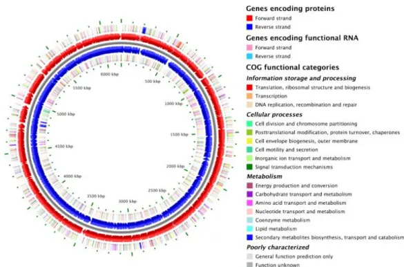
Figure 1 - Circular representation of the Pseudomonas putida KT2440 genome ... 3

Figure 2 - Bioreactor with P. putida KT 2440 cultures after and before suffer stress conditions. The green rectangle represents producing P. putida KT2440 populations, the orange and red rectangle show P-. putida KT2440 subpopulations with reduced and stopped product formation properties, respectively. ... 5

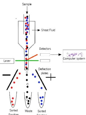
Figure 3 - Schematic diagram of a flow cytometer, showing the fluid sheath, laser, detectors, deflection plates and computer system. ... 6

Figure 4 - Block diagram showing the mass spectrometers components ... 8

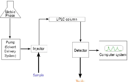
Figure 5 - Block diagram showing the components of an UPLC instrument. ... 9

Figure 6 - Thesis timeline and incorporation into the overall project. ... 11

Figure 7 - Main goal of the overall project. Understand the differences between subpopulations at the same environmental conditions but also at different environmental conditions. ... 11

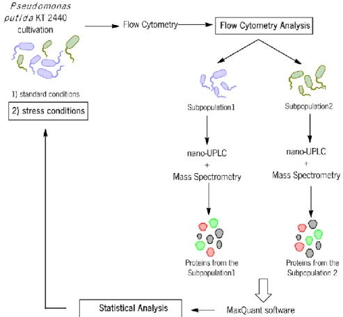
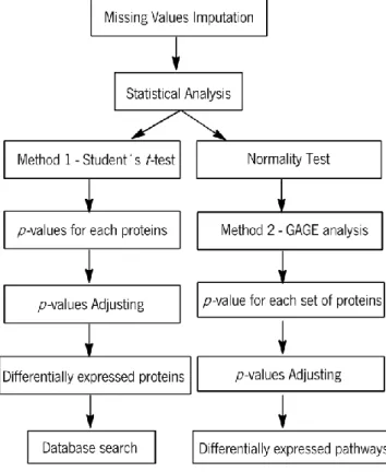
Figure 8 - Work methodology, showing the main steps from the overall project. The rectangles represent the work developed in this thesis. The first stage is the flow cytometry and statistical analysis of the proteomic data from the standard conditions and the second phase is the investigation of different relevant stress conditions. After set-up of the experiments for the stress conditions, these datasets will go through the same cycle of data analysis as the standard conditions. ... 12

Figure 9 - Schematic workflow of statistical analysis... 14

Figure 10 - (A) The plot represents the distribution of the events in the side scatter (SS.Log) and forward scatter (FS.Log) for the 8 samples. Inside the red ellipse are the cells of interest. The rest are debris according to the filter definition. (B) Flow cytometry characterization of P. putida KT 2440 subpopulations, the y-axis represents the samples and the x-axis represents the fluorescence signal captured for the channel 4 (FL.4.Log). ... 22

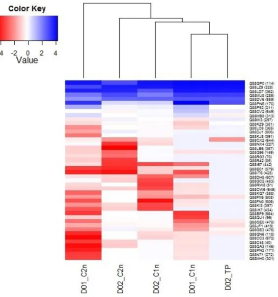
Figure 11 - (A) The plot represents the distribution of the events in the side scatter (SS.Log) and forward scatter (FS.Log) for the 6 samples. Inside the red ellipse are the cells of interest. The rest are debris according to the filter definition. (B) Flow cytometry characterization of P. putida KT 2440 subpopulations, the y-axis represents the samples and the x-axis represents the fluorescence signal captured for the channel 4 (FL.4.Log). ... 23 Figure 12 - Heat Map of up- and down-regulated differentially expressed proteins found in the samples D01_C1n, D01_C2n, D02_C1n, D02_C2n. D02_TP compared with the standard sample (D02_TS). Areas of red represent down-regulated proteins, while blue areas represent up-regulated proteins. Hierarchical clustering separates each sample. Proteins with Uniprot ID are

(9)

sample D07_ CXn. The mean t statistics is the mean of the individual statistics from multiple single array based gene set tests. Red points show differentially expressed and black points commonly expressed pathways. ... 34 Figure 14 - GAGE Mann-Whitney U test analysis. The upper subfigure shows pathways differentially expressed in sample D02_ C1n and the bottom subfigure pathways that are differentially expressed in the sample D02_ TP. The mean MW statistics is the mean of the individual statistics from multiple single array based gene set tests. Red points show differentially expressed and black points commonly expressed pathways. ... 35 Figure 15 - GAGE Mann-Whitney U test analysis. The upper subfigure shows pathways differentially expressed in sample D07_ C2n and the bottom subfigure pathways that are differentially expressed in the sample D07_ CXn. The mean t statistics is the mean of the individual statistics from multiple single array based gene set tests. Red points show differentially expressed and black points commonly expressed pathways. ... 36 Figure 16 - Pulse experiments with (R)-(+) Limonene. Graphic determining the linear regression of the logarithmic optical density of the growth rates before and after each pulse. Plotted is the natural logarithm of the optical density at 600 nm against time. The dashed vertical line marks the time of the pulse. The slope of the regression line drawn in the first four hours and the slope of the regression line drawn after the hour 4 are the growth rates before and after the solvent pulse, respectively. (A) pulse with 0.1 % (v/v); (B) pulse with 0.2 % (v/v) ; (C) pulse with 0.3 % (v/v); (D) pulse with 0.5 % (v/v) of (R)-(+) Limonene. ... 39 Figure 17 - Biomass dry weight. NO STRESS are the shaking flasks without a solvent pulse (standard sample). L 0.1 % represent the shaking flasks with 0.1 % (v/v) , L 0.2 % the shaking flasks with 0.2 % (v/v), L 0.3 %the shaking flasks with 0.3 % (v/v) and L 0.5 % the shaking flasks with 0.5 % (v/v) of (R)-(+) Limonene. * marks significantly different biomass dry weight results from the standard sample (NO STRESS)... 40 Figure 18 - Pulse experiments with α-Pinene. Graphic determining the linear regression of the

logarithmic optical density of the growth rates before and after each pulse. Plotted is the natural logarithm of the optical density at 600 nm against time. The dashed vertical line marks the time of the pulse. The slope of the regression line drawn in the first four hours and the slope of the regression line drawn after the hour 4 are the growth rates before and after the solvent pulse, respectively. (A) pulse with 0.1 % (v/v); (B) pulse with 0.2 % (v/v) (C) pulse with 0.3 % (v/v); (D) pulse with 0.5 % (v/v) of α-Pinene . ... 41

Figure 19 - Biomass dry weight. NO STRESS are the shaking flasks without a solvent pulse (standard sample). L 0.1 % represent the shaking flasks with 0.1 % (v/v) , L 0.2 % the shaking flasks with 0.2 % (v/v), L 0.3 %the shaking flasks with 0.3 % (v/v) and L 0.5 % the shaking flasks with 0.5 % (v/v) of α-Pinene. * marks significantly different biomass dry weight results from the standard sample (NO STRESS). ... 42 Figure 20 - Pulse experiments with Bisabolene. Graphic determining the linear regression of the logarithmic optical density of the growth rates before and after each pulse. Plotted is the natural logarithm of the optical density at 600 nm against time. The dashed vertical line marks the time of the pulse. The slope of the regression line drawn in the first four hours and the slope of the regression line drawn after the hour 4 are the growth rates before and after the solvent pulse respectively. (A) pulse with 0.1 % (v/v); (B) pulse with 0.2 % (v/v) (C) pulse with 0.3 % (v/v); (D) pulse with 0.5 % (v/v) of Bisabolene . ... 43

(10)

Figure 21 - Biomass dry weight. NO STRESS are the shaking flasks without a solvent pulse (standard sample). L 0.1 % represent the shaking flasks with 0.1 % (v/v) , L 0.2 % the shaking flasks with 0.2 % (v/v), L 0.3 %the shaking flasks with 0.3 % (v/v) and L 0.5 % the shaking flasks with 0.5 % (v/v) of Bisabolene. * marks significantly different biomass dry weight results from the standard sample (NO STRESS). ... 44

(11)

List of Tables

Table 1 - Classification of Pseudomonas putida ... 2

Table 2 - M12 solution composition ... 19

Table 3 - Trace elements solution composition ... 19

Table 4 - Quantification of different subpopulations (cell count) and their fluorescence (mean) in growth rate ranging µ =0.1 h-1 and µ =0.8 h-1. ... 22

.Table 5 - Quantification of different subpopulations (cell count) and their fluorescence (mean) in growth rate µ=0.1 h-1, µ=0.2 h-1 and µ=0.7 h-1. ... 23

Table 6 - Information about the proteins differentially expressed in the D01_C1n sample. ... 28

Table 7 - Information about the proteins differentially expressed of the D01_C2n sample. ... 29

Table 8 - Information about the proteins differentially expressed of the D02_C1n sample. ... 31

Table 9 - Information about the proteins differentially expressed of the D02_C2n sample ... 31

Table 10 - Information about the proteins differentially expressed of the D02_TP sample. ... 33

Table 11 - Summary of the growth rates before and after the pulse procedure with (R)-(+)-Limonene. ... 39

Table 12 - Differences between biomass weight in each concentration tested of (R)-(+) Limonene and the standard sample (NO STRESS). The p-values from the statistical analysis can also be found in this table. ND means not significantly different compared to the standard sample (NO STRESS). ... 40

Table 13 - Summarized growth rates before and after the pulse procedure with α-Pinene ... 42

Table 14 - Differences between biomass weights in each concentration tested of α-Pinene and the standard sample (NO STRESS). The p-values from the statistical analysis can also be found in this table. ... 42

Table 15 - Summarized growth rates before and after the pulse procedure with Bisabolene. ... 43

Table 16 - Differences between biomass weights in each concentration tested of Bisabolene and the standard sample (NO STRESS). The p-values from the statistical analysis can also be found in this table. ... 44

Table 17 - Number of proteins for each pathway for the GAGE analysis.- ... 55

Table 18 - Number of p-values before and after the p-values adjustment for each sample (method 1). Additionally, false positive findings of differentially expressed genes are quantified. ... 57

Table 19 - Number of p-values before and after the p-values adjustment for each sample (method 2 using the t-test). Additionally, false positive findings of differentially expressed genes are quantified. ... 57

(12)

Table 20 - Number of p-values before and after the p-values adjustment for each sample (method 2 using the Mann–Whitney U test). Additionally, false positive findings of differentially expressed genes are quantified. ... 58

(13)

1. Introduction

A well producing bacterial population which is exposed to stress conditions may convert to subpopulations with reduced or even stopped product formation properties. Since inefficiently producing subpopulations of Pseudomonas putida cultures may have significant impact on productivity of industrial cultures, it is important to quantify population heterogeneity and find strategies to attenuate it (Müller et al. 2010).

This master thesis addresses particularly the proteomic analysis of P. putida KT2440 continuous cultures to investigate the differences between the subpopulations at varying growth conditions. Results may lead a step towards targeted optimization methods with a new perspective on preventing the advent of subpopulation split-up resulting in a loss of productivity in industrial fermentation processes.

This thesis is organized in four chapters. This introductory chapter that includes a brief description of the state of the art about P. putida and its importance in Biotechnology, biofuels, and stress, cellular heterogeneity, the evolution of proteomic analysis, the motivation of this work and the research aims. Chapter 2 describes the material and methods used for the experimental part and the work flow used for the computational part. Results are presented and discussed in chapter 3 and the conclusions and future perspectives are presented in chapter 4.

1.1 Pseudomonas putida

P. putida is a rod-shaped, flagellated, gram-negative and saprophytic bacterium (Table 1). It is able to colonize different environments such as soil, fresh water and the surfaces of living organisms, e.g. plant roots and the surrounding environments (rhizosphere). It is one of the best studied species of the genus Pseudomonas with an extraordinary diversity of enzymes, metabolic degradation pathways and transporters for secondary metabolites. Furthermore, it is able to tolerate moderate to high solvent concentrations in its environment and has promoting effects on plant growth and protection from pathogens (Espinosa-Urgel et al. 2000). This wealth of interesting properties makes it applicable in various different biotechnological applications including bioremediation of contaminated areas (Kenneth N Timmis et al. 1994) and the

(14)

biocatalytic production of fine chemicals (A Schmid et al. 2001; Zeyer et al. 1985). Other applications are e.g. quality improvement of fossil fuels (Galán et al. 2000), the production of bioplastics, especially polyhydroxyalkanoic acids (PHA) (Olivera et al. 2001), and as agents of plant growth promotion and plant pest control (O’Sullivan and O’Gara 1992; Walsh et al. 2001).

P. putida is an organism that plays a role in various biotechnological fields, ranging from industrial production of chemicals (white biotechnology), medical biotechnology (red biotechnology) and also environmental biotechnology (green). Besides these different applications, P. putida is characterized by stress resistance, can be easily isolated, and is an excellent host for gene cloning and expression, making it well suitable for laboratory experiments and optimization processes. This bacterium holds a few distinctions, including being the first Gram-negative soil bacterium to be certified as a safety strain by the Recombinant DNA Advisory Committee in 1982 (Federal Register 1982).

Table 1 - Classification of Pseudomonas putida.

Domain Bacteria Phylum Proteobacteria

Class Gamma proteobacteria Order Pseudomonadales Family Pseudomonadaceae Genus Pseudomonas

Species Pseudomonas putida

1.1.1 Pseudomonas putida KT2440

The species Pseudomonas putida includes several strains, e.g. P. putida KT2440. This strain was sequenced and annotated in 2002. It contains a single circular chromosome of 6,181,863 bp with an average G+C content of 61.6%, carrying 5420 open reading frames (ORFs) (K. E. Nelson et al. 2002) (Figure 1).

P. putida KT2440 is a plasmid-free derivative of a toluene-degrading strain, initially named Pseudomonas arvilla mt-2 (Kojima et al. 1967) and later designated as Pseudomonas putida mt-2 (Olivera et al. 2001; Williams and Murray 1974).

(15)

Figure 1 - Circular representation of the Pseudomonas putida KT2440 genome (Stothard et al. 2005).

P. putida KT2440 revealed a close evolutionary relationship with P. aeruginosa, one of the most dangerous opportunistic human (Stover et al. 2000) and plant pathogenic Pseudomonas. The genomic similarity between the two species accounts for 77.3 %. The main difference between P. putida KT2440 to P. aeruginosa is the lack of virulence genes. The similarity between P. aeruginosa and P. putida can be an advantage because discoveries made in P. putida might be able to be extrapolated to P. aeruginosa without having to manipulate this dangerous organism.

On a metabolic level P. putida is a versatile bacterium with a very complex metabolism including a large number and diversity of enzymes, transporters and proteins that protect this bacterium against toxic products and enables it to survive in different environments. Interesting pathways that exist in P. putida KT2440 are the catabolic degradation of aromatic compounds. P. putida is able to modify the structure of aromatic compounds, e.g. derived from plant material, into common intermediates of the central metabolic pathway that can be used as carbon and energy sources.

1.1.2 Stress and Biofuels

P. putida strains are known for being solvent-tolerant bacteria (Nicolaou et al. 2010) but the mechanisms and their interplay responsible for this tolerance are still to be understood.

(16)

Biofuels can be produced by microorganisms, but they can cause cellular stress leading to cellular heterogeneity harming the industrial production of these interesting compounds.

α-Pinene, (R)-(+)-Limonene and Bisabolene are considered next-generation biofuels

because they can serve as precursors to produce fuel using suitable microorganisms. These solvents offer many advantages and might supplement existing petroleum fuels in the future. To reach this goal, a suitable industrial host is needed.

P. putida is one cell factory that can be a candidate as a biofuel-tolerant host strain. Therefore, in this thesis, first trial experiments for testing its tolerance towards α-Pinene,

(R)-(+)-Limonene and Bisabolene are studied to pave the way to further investigate these stress conditions at single cell proteome level.

1.2 Cellular Heterogeneity

Since the publication of P. putida KT2440's genome (K. E. Nelson et al. 2002), and the genome-scale model reconstructions (Nogales et al. 2008; Puchałka et al. 2008; Sohn et al. 2010) our knowledge about this bacterium increased significantly. However, many mechanisms of adaptation, stress tolerance or recovery remain unknown and need to be studied.

It is now known that cell behavior differs even under identical micro-environmental conditions (Jahn et al. 2012) resulting in cell heterogeneity. This phenomenon can be caused by stress conditions, for example, in the bioreactors during fermentation processes. It can transform a well producing bacterial population in subpopulations with reduced or even stopped product formation properties (Figure 2). So far this diversity in cell cultures is associated with gene loss, mutations or variations in reactor environments (Fritzsch et al. 2012; Schweder et al. 1999) that can cause epigenetic modifications, variance in cell size owing to asymmetric cell division or different growth (Jahn et al. 2012). It is necessary to understand population heterogeneity because it has a significant impact on the productivity of industrial cultures.

(17)

To obtain more information about population heterogeneity the use of sophisticated techniques is required, such as a combination of fluorescence activated cell sorting (FACS) and mass spectrometry (MS) resulting in proteomic information on subpopulation level rather than on whole population level.

The population elected for the proteomic analysis was Pseudomonas putida KT 2440 because of their biotechnological applicability, their versatile and non-pathogenic characteristics.

1.2.1 Identification of Subpopulations

Flow cytometry is a powerful technique to analyze different parameters of individual cells within heterogeneous populations. Thousands of cells pass through a laser beam per second and the light that emerges from each cell is captured.

The flow cytometer consists of a fluidic system, lasers, optics, electronic parts and a computer system. In the fluidic system, a central channel through which the sample is injected is enclosed by an outer sheath that contains a faster flowing fluid. Lasers are light sources for scatter and fluorescence. The optics receives the light and the electronics and the computer system convert the signals from the detectors into digital data (Figure 3).

When the cell passes through the laser, light is refracted and scattered. Light scatter is collected at two angles: forward scatter (FSC) and side scatter (SSC). Forward scatter measures scattered light in the direction of the laser path and measures the size of the cell and the side scatter measures scattered light at 90 degrees to the laser path and gives information about the granularity of the cell.

Figure 2 - Bioreactor with P. putida KT 2440 cultures after and before suffer stress conditions. The green rectangle represents producing P. putida KT2440 populations, the orange and red rectangle show P. putida KT2440 subpopulations with reduced and stopped product formation properties, respectively.

(18)

One of the big advantages of this system is the fact that flow cytometers can detect very small particles (cells between 1 and 15 microns in diameter), which is a prerequisite for successful realization of prokaryotic population analysis.

To study cellular characteristics, flow cytometry is combined with fluorophore analysis and flow cytometry based cell sorting (FACS). A fluorophore, 4',6-diamidino-2-phenylindole (DAPI), is used to stain DNA. It is a fluorescent stain that binds strongly to A-T rich regions in DNA. DAPI can pass through an intact cell membrane. Therefore it can be used to stain both live and fixed cells. Previous staining of the samples with DAPI allows to measure DNA content of each single cell that passes through the fluorescence cytometer because during the flow cytometry process the DAPI are excited and emit a specific light that will be captured by a specific detector called channel 4 (FL 4). DNA content gives information on which cell in the whole populations is in which state of the cell cycle.

DNA content is then used as a parameter for fluorescence activated cell sorting to separate subpopulations, as the DNA molecule is very stable and it is easily labeled. The analysis of flow cytometry data will be carried out in this thesis using Bioconductor (R. C. Gentleman et al. 2004).

Figure 3 - Schematic diagram of a flow cytometer, showing the fluid sheath, laser, detectors, deflection plates and computer system.

(19)

After separating P. putida KT 2440 in subpopulations, a detailed investigation is necessary of their characteristics and one appropriate approach is studying the proteomics of these cells.

1.3 Proteomics

Proteomics refer to the study of the proteome. The term proteome was defined as the entire set of proteins expressed by the genome. In detail, it is the set of proteins expressed at time of sampling under defined environmental conditions. Nowadays, proteomics is much more than this description. It is considered as all protein isoforms and modifications in a cell, and also the interactions between them, their structural description and their higher-order complexes (Tyers and Mann 2003). Proteins are an important key-element of life because they are the main components of the physiological pathways of the cells. Proteins represent about 50% of dry weight of a prokaryotic organism, catalyze biochemical reactions (enzymes), act as messengers and control elements that regulate cell reproduction, influence growth (growth factors), transport specific molecules and ions (hemoglobin), give organisms the ability to contract, to move or to change their shape, etc.

1.3.1 Proteomic Analysis

Proteomic analysis is the qualitative and quantitative investigation of the proteome. On a qualitative level, it allows to identify proteins, understand their distribution, posttranslational modifications, interactions between them and their structure and function. On a quantitative level it gives information about protein abundance and distribution, temporal changes in abundance due to synthesis and degradation or both and protein stoichiometry of reactions. The understanding of these mechanisms could be revolutionary on an industrial and medical level as it might allow optimization of the production of valuable compounds and can help to obtain information on disease development in an organism.

The method used to study the proteome of the different subpopulations in this project was mass spectrometry (MS).

MS was described by physicists in the late 1880s. It is a technique based on the formation of gas-phase ions from the analyte (positively or negatively charged), realized by the ion source component of the spectrometers. Ions can be isolated electrically (or magnetically) based on their mass-to-charge ratio (m/z) detected by the mass analyzer component. In a MS spectrum, the x- coordinate represents m/z values, whereas the y-axis indicates total ion counts

(20)

(El-aneed et al. 2009). The last part of the mass spectrometers is the ion detector to monitor the ions (Figure 4).

Figure 4 - Block diagram showing the mass spectrometers components (El-Aneed et al. 2009).

Mass-spectrometry-based proteomics is a high-throughput, sensitive and specific analysis for qualitative and quantitative applications that has become an important analytical tool in biology during the past 20 years. Driven by the genome sequencing projects including the human genome (Human Genome Project (Lander et al. 2001)), the success of protein MS was enabled by the development of efficient algorithms to extract data and the development of soft protein ionization methods.

Protein MS needs a high performance separation instrumentation to perform efficient separation of complex mixtures and prepare the molecules for the ionization source leading to high accuracy and sensitivity of the mass spectrometric analysis. The method chosen for the separation of complex peptides and proteins in this project was ultra-high performance liquid chromatography (UPLC).

UPLC is a variant of high-performance liquid chromatography (HPLC) using columns with particle size <2 µm (typically, 1.8 µm). It provides significantly better separation, peak capacity, speed, resolution and sensitivity for analytical determinations, particularly when coupled with mass spectrometers capable of high-speed acquisitions (Churchwell et al. 2005).

The UPLC device includes a sampler that brings the sample from the mobile phase into the stationary phase, pumps that deliver the desired flow and composition of the mobile phase through the column, the detector that generates a signal proportional to the amount of sample component emerging from the column, and the computer system, which controls the UPLC instrument and provides data analysis (Figure 5).

(21)

Figure 5 - Block diagram showing the components of an UPLC instrument.

Overall, the combination of fluorescence labeling, fluorescence activated cell sorting and UPLS+MS allows a separation of different subpopulations and getting the proteomic profiles of each subpopulation in order to give insights into molecular heterogeneity.

1.3.2 The MS Raw Data Analysis

After successful realization of MS experiments, algorithms need to be applied to extract information for analysis of mass spectrometry data in an efficient and robust way. Several thousand proteins in complex proteomes need to be identified and quantified with high-accuracy.

Known algorithms for the use in proteomic analysis are: ASAP Ratio (X.-J. Li et al. 2003), AYUMS (Saito et al. 2007), Census (S. K. Park et al. 2008), i-Tracker (Shadforth et al. 2005), jTraqX (Muth et al. 2010), MaxQuant (Cox and Mann 2008), MRmer (Martin et al. 2008), MSQuant (Mortensen et al. 2010), XPRESS (Han et al. 2006).

The algorithm used in this work with the cooperation of a partner UfZ Leipzig was MaxQuant, a quantitative proteomics software package designed for analyzing large mass spectrometric datasets. It is specifically aimed at high-resolution MS data. MaxQuant was developed at Max-Planck Institute for the NET framework and was written in the C# language. The interactive 3D data viewer was developed on the basis of DirectX. MaxQuant detects peaks, isotope clusters and stable amino acid isotope-labeled (SILAC) peptide pairs as three-dimensional objects in m/z, elution time and signal intensity space using correlation analysis and graph theory. It identifies and quantifies peptides and in silico composition of proteins. Each protein will be identified by at least two different peptides and the quantity is calculated by the integration of the peak. The software output is a table with identified proteins and peptides, which will be the basis for this thesis.

(22)

1.3.3 Proteomic Data Analysis

After the raw data analysis the list of all identified and quantified proteins was obtained from the cooperation partner UfZ Leipzig.

To build the basis for meaningful proteomic data analysis, various statistical function and methods must be applied, e.g. standard deviations, missing values imputation, statistical and significance analysis (p-value), gene ontology analysis etc.

One of the most used software in statistical computing and graphics is the R software (R Development Core Team 2012) and specifically the Bioconductor (R. C. Gentleman et al. 2004) for the analysis of high-throughput data.

Bioconductor is a free open source and open development software project built on the statistical freeware R software used for the analysis and comprehension of high-throughput gene expression data, but it can also be applied for another omics data as e.g. proteomics.

1.4 Research aims

This master thesis is integrated in the project: "Deciphering population dynamics as a Key for Process Optimization". The master thesis is divided in two phases: The first one is the proteomic analysis of P. putida KT 2440 cultured in standard conditions. Sarah Lieder established the standard conditions in the lab, and fermentation samples were analysed and sorted via FACS and the subpopulation proteome was analysed via UPLC+MS in the facilities of the cooperation partner UfZ Leipzig. The flow cytometry analysis and statistical analysis of the proteomic data is performed in this thesis and comprises the final part of the investigation of the standard conditions.

The second phase of the overall project is the investigation of different industrial relevant stress conditions. Therefore, as a second phase of this master project, tolerance levels of P. putida to α-Pinene, (R)-(+)-Limonene and Bisabolene are investigated, for a successful

establishment of the experimental set-up of stress conditions on P. putida cultures. The overall project will contain fermentation scale solvent stress investigations on subpopulation level and the statistical analysis platform developed in the first part of the thesis will serve as tool for the analysis of the subpopulation proteomics under stressed conditions. The standard conditions analysed within this thesis will then serve as basis for comparison of non-stressed to stressed

(23)

Figure 6 - Thesis timeline and incorporation into the overall project.

In summary, the main goals of this master thesis are a reliable data analysis of the P. putida subpopulation proteome to understand the differences in subpopulations at the same environmental condition comparing with the total population (Figure 7), but also at varying growth conditions. Additionally, it is tested if DNA content as a sorting criterion for subpopulation proteome analysis is giving insights into differences of subpopulations.

Figure 7 - Main goal of the overall project. Understand the differences between subpopulations at the same environmental conditions but also at varying growth conditions.

During the computational part of the thesis the MaxQuant software, with the cooperation of a partner, will be used to extract information of proteome data and the R software (R Development Core Team 2012) will be used for the statistical analysis to characterize the subpopulation split-up under various controlled steady-state conditions. A statistical analysis platform will be built for the analysis of standard condition data, but also for the analysis of the stress datasets, that will not be part of this project. Within the experimental part, called Shake Flask Experiments, preliminary experiments for the experimental set-up of stress investigation

(24)

experiments are carried out to find tolerance levels towards industrially interesting solvent compounds (Figure 8).

Figure 8 - Work methodology, showing the main steps from the overall project. The rectangles represent the work developed in this thesis. The first stage is the flow cytometry and statistical analysis of the proteomic data from the standard conditions and the second phase is the investigation of different relevant stress conditions. After set-up of the experiments for the stress conditions, these datasets will go through the same cycle of data analysis as the standard conditions.

(25)

2. Material and Methods

2.1. Flow Cytometry Analysis

Flow cytometry is one of the crucial tools available to investigate the behaviour of cell populations. R (R Development Core Team 2012) and Bioconductor (R. C. Gentleman et al. 2004) are used as a platform for analysis and visualization of the original complex multidimensional datasets originating from the flow cytometry output.

In this thesis the flow cytometry datasets of the standard continuous cultivation at different growth rates until wash out of the culture are analyzed. The intention is to find out if there are different subpopulations at varying growth rates and how these subpopulations evolve with increasing growth rate.

The packages chosen to perform the flow cytometry analysis and visualize this datasets were flowCore (Meur et al. 2013), flowViz (B Ellis et al. 2008) and latticeExtra (Deepayan Sarkar and Andrews 2012).

In a first step, the batch of FCS files was loaded into the R workspace to create a flowSet. A flowSet is a series of flowFrames, a meta-object that collects different types of information into a common identifier.

As a second step, the dataset is gated. Gating in flow cytometry is an important process for selecting populations of interest for further analysis and visualization. Noise, noncellular debris, cell debris, or clots of cells need to be removed using the norm2filter function. The gating was performed on forward scatter (FSC) and side scatter (SSC) levels to help ensure that the fluorescent measurements exhibit specificity for the target of interest.

The xyplot and densityplot were the functions used to perform the visualization.

The quantification of the subpopulations was performed using the Cyflogic v.1.2.1 (CyFlo Ltd, PL634, 20701 Turku, Finland).

2.2. Proteomic Data Analysis

Proteomic data analysis was performed on data sets of a continuous cultivation of P. putida KT2440 at standard conditions at various growth rates. Each sample was measured in

(26)

biological duplicates at three different growth rates: a very slow growth rate, µ=0.1 h-1, a standard growth rate at which the continuous cultivations for stress conditions will be carried out in the future µ=0.2 h-1 and finally, the maximal growth rate µ=0.7 h-1. Each sample was sorted into different subpopulations (for details see chapter 1.2.). Additionally the method needs to be checked by an internal standard sample. Here, the total population (TP) of the standard growth rate, both sorted (D02_TS) and not sorted (D02_TP) in the FACS serves as a standard for the method itself. Therefore, in total a number of 8 samples in duplicate were analyzed on proteomic level, generating 679 proteins displays.

The signal intensities of all peaks derived from each group in the mass spectrometer were exported to the MaxQuant software.

The proteomic data produced by MaxQuant were imported into R (version 2.15.1) (R Development Core Team 2012) to perform the statistical analysis. The workflow of statistical analysis is visualized in Figure 9.

Figure 9 - Schematic workflow of statistical analysis.

2.2.1. Missing Values Imputation

(27)

mass-ignore important data or do not take the correlation structure between the data into consideration resulting in harming the downstream analysis. To circumvent these consequences, the missing values imputation was carried out via a technique called k-nearest neighbors (KNN). KNN selects proteins with similar expression profiles to the missing protein to impute the missing value. It was proven to be a sensitive, fast and robust method for missing values estimation (Troyanskaya et al. 2001).

The imputation process of the KNN method is divided into two steps. In the first step, a set of proteins with a similar expression profile to the protein with a missing value is selected. The similarity was calculated via the Euclidean distance because it has been reported to be more accurate (Nguyen et al. 2004) and more sensitive to outliers (Troyanskaya et al. 2001). In the second step the missing values are predicted using a weighted average of the proteins selected in step 1.

KNN imputation was done using the Bioconductor in R computing language with the impute package (Trevor Hastie et al. 2005). Troyanskaya et al. (Troyanskaya et al. 2001) reported the best results for the number of neighbours (k) between 10 and 20. As a consequence of this, k=10 was chosen to perform the KNN method. Missing proteins were imputed by averaging the k nearest neighbour (non-missing) elements. In the event that 50 % neighbours were missing in a particular element, the overall sample mean for that block of proteins was used. In case more than 80 % of the entries were missing in any protein the program reported an error.

2.2.2. Testing the Normal distribution of the data

It is important to test the normality of the data before performing the statistical test to understand protein expression levels mainly because the proteomic data does not always follow a normal distribution (Albaum et al. 2011). This test was used only for the proteome datasets in method 2 (Proteins Set Analysis) because in method 1 (Student's t-test Analysis) the proteome datasets are only available in duplicates.

Therefore, the Shapiro-Wilk test (Shapiro and Wilk 1965) was used on the datasets in the R software (R Development Core Team 2012). A normally distributed population serves as the null hypothesis whereas the not-normally distribution serves as alternative hypothesis. A p-value < 0.05 was considered statistically significant. This data serves as input for further analyses.

(28)

2.2.3. Statistical Data Analysis - Method 1 (Student's t-test Analysis)

Significantly different protein expression between two different groups was determined using Student's t-tests for each protein. Unpaired analyses were used to compare the different samples with the control (D02_TS). To perform this statistical test, first a null hypothesis was stated, “protein not differentially expressed in relation to the standard sample” as well as the alternative hypothesis, “protein differentially expressed in relation to the standard sample”. Based on the values measured and the normality assumption on the probability distribution of the data, either the null or the alternative hypothesis was maintained or rejected. A p-value < 0.05 was considered statistically significant.

2.2.4. Statistical Data Analysis - Method 2 (Proteins Set Analysis)

The proteome datasets are only available in duplicates due to experimental costs. Therefore, the normality of the proteomic dataset cannot be tested and the Student's t-test could be not the best test to estimate differentially expressed proteins. Therefore, an additional strategy was used for statistical analysis, a Gene Set Analysis (GSA). GSA is a powerful strategy to infer functional and mechanistic changes from high throughput microarray or sequencing data based on pathway knowledge.

GSA allows the identification of differentially expressed groups of proteins unlike the method described above that analyses individual differentially expressed proteins. The advantages of this approach are the encompassing of larger amount of biological information helping to interpret the data, the incorporation of biological pathway information, the facilitation to detect biologically important signals and more coherent results (Luo et al. 2009).

The GSA method chosen was a based parametric gene randomization procedure called Generally Applicable Gene-set Enrichment (GAGE). It can be used in datasets with different number of samples (Luo et al. 2009).

GAGE was implemented using the Bioconductor package gage (Luo et al. 2009) in the statistical computing language R.

The first step is the protein set preparation, in which the proteins are separated into two groups: the experimental sets and the set of pathways. The experimental data is the result of the MS analysis and the proteomic annotation. The set of pathways comes from extracted data from

(29)

second step is the differential expression test based on a one-on-one comparison between the two groups. For each pair of the experiment set the differential expression was calculated on a log based fold-change. The differential expressed set of proteins was calculated using two different methods to test the suitability of these methods for proteome data analysis: a parametric two-sample t-test and the non-parametric Mann–Whitney U test. In both statistical tests unpaired analyses were used to compare the different samples with the control sample (D02_TS).

Performing the GAGE analysis with a two sample t-tests, two assumptions on the log based fold changes of the target protein set and control sets are made: the data is approximately normally and independent.

In contrast, the Mann–Whitney U test tries to determine if two datasets differ significantly without the assumption of normality. The null hypothesis was defined as “the set of proteins (pathway) are not differentially expressed compared to the standard sample” and the alternative hypothesis as “the set of proteins (pathway) are differentially expressed in relation to the standard sample”. The same p-value was used as in the Student's t-test (p<0.05).

2.2.5. Adjusting of p-values

To avoid a high number of false positives of differentially regulated proteins/pathways, the p-values were adjusted using an algorithm called "False Discovery Rate" (FDR) (Benjamini and Hochberg 1995). Take the n ordered p-values, p(1) ≤ p(2) ≤ … ≤ p(n)", the FDR-adjusted p-values are given by equation 1.

Equation 1 The adjustment procedures were implemented in the p.adjust method of the R-package “stats” (R Development Core Team 2012) and applied on the two methods described above. The result is a FDR analogue of the p-value, called q-value.

2.2.6. Proteomic Annotation

In order to facilitate the functional annotation and analysis of all proteins, DAVIDQuery (Day and Lisovich 2010), an R Package for retrieving data from DAVID (Database for Annotation, Visualization and Integrated Discovery) (Dennis et al. 2003) into R objects, was used. DAVID helps in visualization of high-throughput data and allows biological annotation (Dennis et al. 2003).

(30)

To get information about the locus tag, protein name, gene name, protein length, function, pathway and subcellular location etc., the protein ID given by the MS was converted into an Entrez gene ID and a Uniprot ID using the function convertIDList from DAVIDQuery (Day and Lisovich 2010). This procedure allowed access to information from the Pseudomonas Genome Database (Winsor et al. 2011) and the Universal Protein Research (Uniprot).

The search for information about the proteins differentially expressed in method 1 was directly carried out in different databases like KEGG (Kanehisa et al. 2012), Uniprot (Consortium 2012) and BIOCYC (Caspi et al. 2008).

For the method 2, extracted data from the database Kyoto Encyclopedia of Genes and Genomes (KEGG) (Kanehisa et al. 2012) was used to characterize the differentially expressed proteins. Differentially expressed proteins found using the locus tag ID were sorted into pathways for easier interpretation of the results.

2.2.7. Heat Map Plots

Visualization methods are very important for the interpretation of high-throughput data. Heat map plots were used to visualize the up or down regulated proteins from the differentially expressed proteins or pathways. The heat maps were drawn using the heatmap.2 function in the gplots package (Gregory R. Warnes, 2013) in R (R Development Core Team 2012).

The rows represent the different proteins or pathways and the columns show the different samples and environmental conditions. The color coding is derived using the fold change values. Shades of blue represent up-regulation and shades of red represent down-regulation. The fold change is a measure used to compare two values of protein expression. Here, it is calculated by taking the logarithm of the ratio of the both expression values, the proteins (Ep) expression values of each sample and the expression values of the standard sample (Es) (Equation 2).

Equation 2

2.3. Shake Flask Pulse Experiments

2.3.1. Organism and Media

(31)

Stock solutions of trace elements, glucose and phosphate buffer were prepared and separately autoclaved to simplify media preparation.

The phosphate buffer stock solution was prepared dissolving 100 g of KH2PO4 in 1 L of distilled water. A pH of 6.7 was adjusted using KOH pills.

Table 2 - M12 solution composition and concentration in the final cultivation media.

Composition Weight [g] per 1 L Concentration (g/L)

(NH4)2SO 22 0.4

NaCl 0.2 0.02

MgSO4.7 H20 4 0.4

CaCl2.2 H20 0.4 0.04

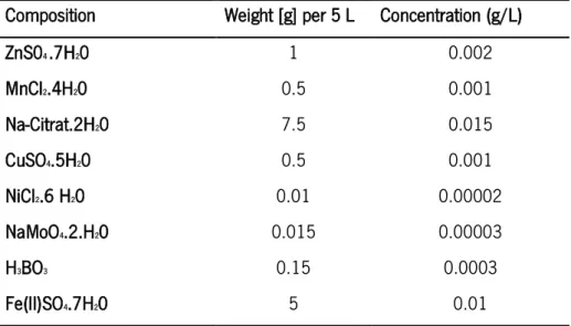
Table 3 - Trace elements solution composition and concentration in the final cultivation media.

Composition Weight [g] per 5 L Concentration (g/L)

ZnS04 .7H20 1 0.002 MnCl2.4H20 0.5 0.001 Na-Citrat.2H20 7.5 0.015 CuSO4.5H20 0.5 0.001 NiCl2.6 H20 0.01 0.00002 NaMoO4.2.H20 0.015 0.00003 H3BO3 0.15 0.0003 Fe(II)SO4.7H20 5 0.01 2.3.2. P. putida KT 2440 cultivation

P. putida KT 2440 cultures were grown at 30º in 500 mL shake flasks in a horizontal rotary shaker at 180 rpm at a working volume of 50 ml. Cultures were grown for 4 hours, until they reached the exponential growth phase. At 4 hours of cultivation time, a pulse of a solvent with a specific concentration was given. Before the pulse, samples were taken every hour, after the pulse every 30 minutes, to monitor growth behaviour. The experiment was stopped after 7 hours and the biomass dry weight was determined (see section 2.3.3) The compounds used in this thesis were α-Pinene, (R)-(+) Limonene and Bisabolene at the concentrations of 0.1 %, 0.2 %, 0.3 %, 0.4 % and 0.5 % (v/v).

(32)

2.3.3. Biomass measurements

Biomass was monitored using two different methods.

The optical density can serve as a measure of the biomass concentration of the cultivation broth. This spectroscopic measurement is carried out at a wavelength of 600 nm in a Photometer Ultrospec 1100 pro (Amersham Biosciences) using polystyrol cuvettes (SARSTEDT). This measurement does not need a high volume of cultivation broth and therefore served as a biomass measurement to monitor the growth trajectory throughout the shake flask cultivation. To get a direct measurement of the biomass concentration, the biomass dry weight was measured at the end of each cultivation. Triplicates of aliquots of 10 mL of P. putida suspension were centrifuged and the pellet was dried at 95º C during 24 hours. The glass tubes with the dried pellets were cooled down in a vacuum desiccator for at least 2 hours, and then weighed. The weight difference of the empty glass tube to the glass tube with the dried pellet equals the biomass dry weight in 10 mL cultivation broth.

2.3.4. Statistical Analysis

The statistical analysis for the pulse experiments was performed using SigmaPlot 11.0 with the Holm-Sidak Multiple Comparison Test.

(33)

3. Results and Discussion

3.1. Flow Cytometry Analysis

Flow cytometry analysis was performed according to the procedure described in section 2.1. Samples for various growth rates from a chemostat experiment under standard conditions ranging from µ=0.1 h-1 to µ=0.8 h-1 were investigated.

Using a density plot to visualize the distribution of the events in the side scatter (SSC) and forward scatter (FSC) it is possible to realize that with increasing growth rate cells are getting bigger (Figure 10).

To get information on DNA content of the populations, the cells were stained with DAPI as mentioned in section 2.1. The fluorescence signal corresponds to the quantity of the DNA in each single cell of the population. To be able to identify subpopulations, a histogram view of the gated data was plotted (Figure 10).The quantification of the subpopulations was provided by Cyflogic v.1.2.1 (CyFlo Ltd, PL634, 20701 Turku, Finland) after plotting an histogram that display a single measurement parameter (fluorescence) on the x-axis and the number of events (cell count) on the y-axis (Table 4).

In the growth rates between µ=0.1 h-1 and µ=0.6 h-1 two different subpopulations of P. putida KT2440, that were called the subpopulation 1 (C1n) and subpopulation 2 (C2n) were found. The subpopulation 1 has one chromosome equivalent whereas the subpopulation 2 has two chromosome equivalents meaning that the subpopulation 1 is in the growth phase shortly after division and just about to start replicating and the subpopulation 2 is in the pre-division phase after finishing replication.

In the very fast growth rates (µ=0.7 h-1 and µ=0.8 h-1) subpopulation 2 (C2n) and a subpopulation called CXn, where replication and division are uncoupled resulting in multiple chromosome containing cells can be found. The uncoupled cell cycle is found in some bacteria species growing at very fast growth rates.

Furthermore, the analysis of the DNA histogram (Figure 10) and Table 4 show that with increasing growth rate the subpopulation 2 increases, and subpopulation 1 decreases (µ=0.1 h-1

(34)

to µ=0.6 h-1) (Table 4). Subpopulation 1 vanishes at growth rates higher than µ=0.7 h-1 and the CXn subpopulation is evolving.

Figure 10 - (A) The plot represents the distribution of the events in the side scatter (SS.Log) and forward scatter (FS.Log) for the 8 samples. Inside the red ellipse are the cells of interest. The rest are debris according to the filter definition. (B) Flow cytometry characterization of P. putida KT 2440 subpopulations, the y-axis represents the samples and the x-axis represents the fluorescence signal captured for the channel 4 (FL.4.Log).

Table 4 - Quantification of different subpopulations (cell count) and their fluorescence (mean) in growth rate ranging

µ =0.1 h-1 and _µ =0.8 h-1.

Cell count (%) Fluorescence FL-4 (mean) Samples C1n C2n CXn C1n C2n CXn GR 0.1 77.4 22.6 - 34.5 61.5 - GR 0.2 61.4 38.6 - 33.9 59.4 - GR 0.3 50.0 50.0 - 32.9 56.2 - GR 0.4 22.2 77.8 - 33.8 59.2 - GR 0.5 17.9 82.1 - 43.8 58.7 - GR 0.6 15.3 28.7 - 45.7 62.3 - GR 0.7 - 41.8 58.2 - 58.4 81.3 GR 0.8 - 41.5 58.5 - 60.9 87.7

(35)

For complete analysis of the standard conditions and to get information about the proteomic content of different subpopulations at different growth rates, the very slow, µ=0.1 h-1, and a very fast growth rate, µ=0.7 h-1, were chosen for further investigation to get the proteomic composition of all 3 subpopulations found: C1, C2 and CX. As a reference for the slow and fast growth rates and to be able to compare the stress condition experiments that will be carried out in the future, the dilution rate µ=0.2 h-1 was also investigated.

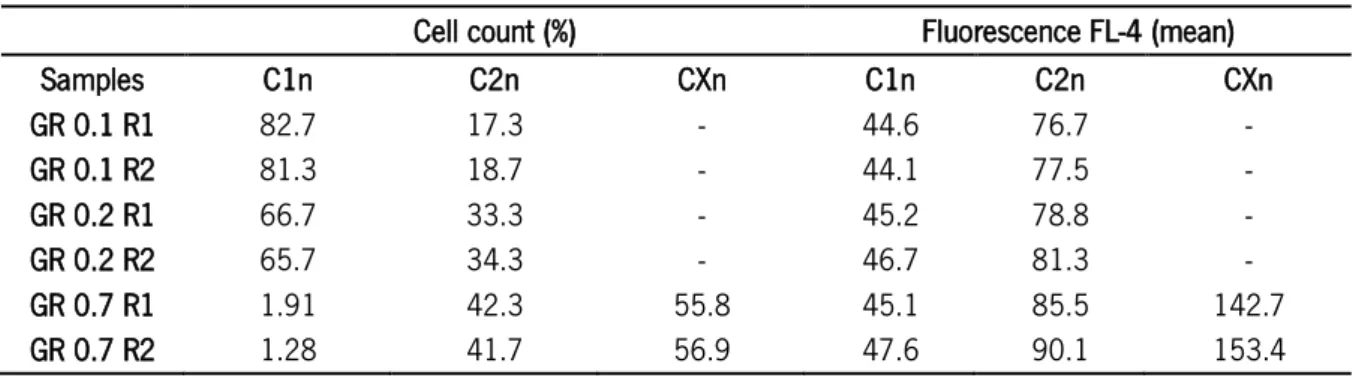
Figure 11 - (A) The plot represents the distribution of the events in the side scatter (SS.Log) and forward scatter (FS.Log) for the 6 samples. Inside the red ellipse are the cells of interest. The rest are debris according to the filter definition. (B) Flow cytometry characterization of P. putida KT 2440 subpopulations, the y-axis represents the samples and the x-axis represents the fluorescence signal captured for the channel 4 (FL.4.Log).

Table 5 - Quantification of different subpopulations (cell count) and their fluorescence (mean) in growth rate µ=0.1 h -1, _µ=0.2 h-1 and _µ=0.7 h-1.

Cell count (%) Fluorescence FL-4 (mean) Samples C1n C2n CXn C1n C2n CXn GR 0.1 R1 82.7 17.3 - 44.6 76.7 - GR 0.1 R2 81.3 18.7 - 44.1 77.5 - GR 0.2 R1 66.7 33.3 - 45.2 78.8 - GR 0.2 R2 65.7 34.3 - 46.7 81.3 - GR 0.7 R1 1.91 42.3 55.8 45.1 85.5 142.7 GR 0.7 R2 1.28 41.7 56.9 47.6 90.1 153.4

(36)

3.2. Proteomic Data Analysis

3.2.1. Missing Values Imputation

31 % of missing values were found in the datasets of the 8 investigated samples (679 proteins). In the case of 190 proteins more than 50 % of the entries were missing. In these cases, as mentioned in section 2.2.1, the KNN method was performed to calculate the overall mean per sample.

3.2.2. Adjusting of p-values

The results of the analysis of differentially expressed proteins for the Student´s t-test and for the Protein Set Analysis method before and after the FDR adjustment can be found in the attachment.

3.2.3. KEGG analysis

The KEGG analysis (section 2.2.6) served as a preparation for the GAGE analysis. The KEGG file contains 2531 proteins, but only 1494 are unique proteins. On this file, just 407 were mapped and used for the output file for the protein set analysis. Having a total number of 679 proteins displays from the MS, the percentage of proteins analyzed in the GAGE method is approximately 60 %.

The table with the number of proteins distributed by 94 pathways that serves as a basis for further investigations in this thesis can be found in the attachment.

3.2.4. Normal distribution analysis

Testing the normal distribution is important to be able to choose a suitable statistical test for the application on ones dataset. For the test at least triplicate datasets need to be available. The proteomic data is only available in duplicates, as mentioned earlier. Therefore, this test was not used in the original data, but just for the data used for the GAGE analysis. The test was performed as explained in section 2.2.2.

For the normal distribution analysis 71 pathways were used from the original file. 23 pathways were removed, as they contained only one protein.

(37)

normal distribution (Albaum et al. 2011). This result confirms the need for a normality test previous to proteomic statistical analysis.

3.2.5. Statistical Data Analysis – Method 1 (Student's t-test Analysis)

To understand the proteomic differences in between the subpopulations and in between different growth rates, it is crucial to understand the behavior of P. putida KT2440 as a population inside a bioreactor. The information of the statistical analysis of P. putida cultivated in a standard environment serves as a basis for further investigations on stress levels. The results will help to investigate Pseudomonas' ability to manage, to adapt and to recreate after being exposed to production-like stress conditions. The choice of a suitable statistical method to understand the proteomic data is crucial, as it can dramatically affect the results, in detail the selection of differentially expressed proteins. Two different methods were applied, as described in detail in section 2.2.3. In this chapter the results of the two methods are described and discussed, as well as the methods themselves are explored and evaluated.

The statistical data analysis was performed for a quantification of differences between the subpopulations at the different growth rates in comparison to the standard total population (D02_TS).

Using the Students t-test, at a slow growth rate of µ=0.1 h-1 (D01), 3 differentially expressed proteins were found in subpopulation 1 (D01_C1n) and 21 in subpopulation 2 (D01_C2n), respectively. It represents 0.4 % and 3.1 % of changed proteins in the subpopulation with one chromosome equivalent (D01_C1n) and in the subpopulation with two chromosome equivalents (D01_C2n), respectively when comparing to the standard sample (D02_TS).

At a growth rate of µ=0.2 h-1 (D02), 13 differentially expressed proteins for subpopulation 1 (D02_C1n), 16 for subpopulation 2 (D02_C2n) and 1 single protein for the control total population sample (D02_TP) were found. This corresponds to a difference of 1.9%, 2.4% and 0.1% between the samples D02_C1n, D02_C2n and D02_TP comparing with the standard sample (D02_TS), respectively.

At a growth rate of µ=0.7 h-1 (D07) 267 differentially expressed proteins were discovered in subpopulation 2 (D07_C2n) and 53 in the subpopulation with a multifold chromosome content X (D07_CXn). These results represent 39% of differentially expressed proteins of subpopulation 2 (D07_C2n) compared to the standard sample (D02_TS), and 7.8% of difference in protein expression between the multifold DNA content subpopulation (D07_CXn) and D02_TS.

(38)

In case of the third growth rate µ=0.7 h-1, the different proteins are not directly looked up for detailed research in protein databases, as the search and interpretation of this high number of proteins would not lead to a targeted interpretation of the changes. Therefore, another test was performed called Generally Applicable Gene-set Enrichment (GAGE).

Discovering differentially expressed proteins is important to find optimization targets for e.g. improved stress tolerance or the production of an interesting compound. To draw conclusions for metabolic engineering strategies, it is not only important to find differentially expressed proteins, but also to quantify down or up-regulation. This information cannot be derived directly from the t-test analysis. Therefore, a heat map for visualization of fold-changes was constructed with all proteins differentially expressed for growth rates µ=0.1 h-1 and µ=0.2 h-1. Looking only at the fold change does not take the variance of the expression values measured into consideration. Therefore, it should be used only in combination with statistical methods (Tarca et al. 2008). For this reason, the Student t-test was applied in this thesis, before investigating fold-changes. In summary, proteins that were found to be differentially expressed in subpopulation 1 at a slow growth rate of µ=0.1 h-1 were all down-regulated proteins. The same picture is found looking at subpopulation 2, given one up-regulated exception (protein 170). This trend continues in the other samples investigated (µ=0.2 h-1, subpopulation 1 and 2). Most of the proteins found to be differentially expressed are down-regulated. In subpopulation 1, only three regulated proteins could be found (114, 328 and 589) whereas in subpopulation 2 five up-regulated proteins (285, 328, 362, 589 and 649) could be identified.

One protein was found to be down-regulated in the control sample (D02_TP). The visualization of these results can be seen in the heat map plot in Figure 12.

(39)

Figure 12 - Heat Map of up- and down-regulated differentially expressed proteins found in the samples D01_C1n, D01_C2n, D02_C1n, D02_C2n. D02_TP compared with the standard sample (D02_TS). Areas of red represent down-regulated proteins, while blue areas represent up-regulated proteins. Hierarchical clustering separates each sample. Proteins with Uniprot ID are indicated on the right of the figure.

Another important information that can be drawn out of this analysis is the proteins differentially expressed in common between the subpopulations of each growth rate. Common changes in proteome of both subpopulations compared to a different growth rate can be concluded to occur due to the change of the growth rate. One common protein at a growth rate of µ=0.1 h-1 and four common proteins at a growth rate of µ=0.2 h-1 could be detected. Detailed information on the proteins found, their biological function and the interpretation of these results can be found in the following paragraphs. The proteins found to be differentially expressed are summarized in the following set of tables and described and discussed in the following paragraphs.

(40)

At a growth rate of µ=0.1 h-1 the DNA topoisomerase was found to be down-regulated, (Table 6). DNA topoisomorase has the function to release the supercoiling and torsional tension of DNA introduced during the DNA replication and transcription by transiently cleaving and rejoining one strand of the DNA duplex. The decrease in protein quantity at a low growth rate fits the expectation. The cell adjusts the speed of replication and division to the slow growth rate. The other two proteins differentially expressed in this sample do not have an annotated function. Therefore, at this point, it is not possible to draw any conclusion about these proteins. In general it can be concluded that there is not a significant change in the proteome at a difference of growth rates from µ=0.1 h-1 to µ=0.2 h-1 between subpopulation 1 and the total standard population (D02_TS).

Table 6 - Information about the proteins differentially expressed in the D01_C1n sample.

ID q-value Uniprot Entrez Protein name Length Regulation 99 0,043 Q88QU1 1044108 Putative uncharacterized

protein 522 Down regulated 381 0,043 Q88KZ9 1044994 DNA topoisomerase 869 Down regulated 564 0,003 Q88EF9 1041845 Nitroreductase family

protein 185 Down regulated

In subpopulation 2 proteins were differentially down-regulated in nucleotide metabolism (40,146), amino-acid biosynthesis (171,211,297), ribosome pathway (118), glycolipid biosynthesis for membrane biogenesis (272, 301, 597) and the bacterial secretion system (434) (Table 7). These results can again be connected to the slow growth rate. Subpopulation 2 already finished replication of DNA in comparison to subpopulation 1. In comparison to the faster growing population at D=0.2 h-1 the amount of “building blocks” like amino-acids to integrate into proteins, nucleotides for the replication, ribosome enzymes for the translation machinery or lipids for the membranes are less needed.

Generally, the changes of the proteomic profile in subpopulation 2 at a growth rate of D=0.1 h-1 are bigger than in subpopulation 1 comparing to the standard population at a growth rate of D=0.2 h-1.