Implementation of
α
-QSS Stiff Integration
Methods for Solving the Detailed Combustion
Chemistry
Shafiq R. Qureshi and Robert Prosser
Abstract— Implicit methods for reacting flow systems are
considered efficient when expressed in terms of a time step length. A drawback of these methods is the additional work required at each time step for solving the sparse matrix of algebraic equations, which degrades their efficiency. Explicit methods are easy to implement but require excessively small steps. Predictor-corrector methods are another option, which utilise the concepts of both implicit and explicit methods. A recently proposed α-QSS (quasi steady state) method is an example of a second order predictor-corrector A-stable method. In the present study we carry out integration of a one dimensional laminar methane flame. During the integration of the methane mechanism the method requires small time steps where concentrations are rapidly varying. In the pre-heat and equilibration periods, the method is not efficient and unnecessarily takes smaller steps. An alteration is proposed in the convergence criteria which improves the efficiency of the method in the pre-heat and equilibration zones, and which results in a reduction in the computation time by a factor of 15. Due to the small time step, the temperature change at each step is also small, so an additional time saving can be achieved if rate coefficients are calculated only after a predetermined change in temperature.
Index Terms— Combustion, Implicit Methods, Reacting Flows, Stiff integration,
I. INTRODUCTION
Combustion is the main source of energy for applications such as transportation, heating and electrical energy production [1]. More than 80% of worldwide energy requirements are met by the combustion of organic fuels [2]. High consumption of these fuels has increased the level of green house gases (GHG) in the atmosphere. The emission of CO2 in
particular has increased in the last decade significantly [3]. An increased awareness of the environmental impact of combustion emissions has led industries to seek detailed fundamental knowledge of the combustion process.
Combustion is a complex phenomenon, in which fluid dynamics, chemical reactions and subsequent heat release are closely related. The solution of such a flow system requires the simultaneous solution of coupled physics. Normally, process splitting (or operator splitting) techniques are used to address this problem [4]. In this technique, the
Manuscript received October 9, 2006. (Write the date on which you submitted your paper for review.)
Shafiq R. Qureshi is with the University of Manchester, e-mail: s.qureshi@ postgrad.manchester.ac.uk).
Robert Prosser is with University of Manchester, e-mail: [email protected]).
effects of individual processes are calculated separately for a predefined global time step and then the results are combined in some way. Production and consumption of different species during the combustion process present a highly non linear phenomenon. The reaction time scales differ significantly in different elementary reactions resulting in a stiff set of differential equations. The temporal integration of such equations need very small time steps to obtain an accurate solution. This situation requires the use of expensive implicit solvers [2], which typically require the solution of large algebraic systems of equations at each time step. Typically in the simplest H-O combustion model, more than 95% of time of the total calculations is used for chemistry calculation [5].
The purpose of the present study is to establish whether α-QSS stiff integration methods can be used to reduce the cost of laminar flame calculations. The global time step in a flame is governed by the fastest timescales in the chemical reaction. Hence, our study will apply the α-QSS approach to individual sections of the flame. In this way, we can clearly see which parts of the flame structure demand the shortest time step. Furthermore, the results of the simulations will inform us of the maximum time step we should be able to use.
In the remainder of this paper, we employ an A-stable quasi steady state (QSS) method for integrating reaction kinetics, and which was proposed by Mott et al [9,11]. In our calculation we have simulated a methane reaction mechanism comprising 68 reactions and involving eighteen species. A slight modification in the method’s convergence criteria is proposed, which has produced improved results with a slight accuracy loss in the cold zone and the equilibration zone.
II.
STIFFNESS
Stiffness occurs in problems when the rates of change of two or more dependent variables of the same system differ by a large ratio. In practical computations a system is stiff if the step size, expressed in terms of cost or running time is too large to give a stable, accurate solution. Mathematically, a system is stiff when the Jacobian matrix has eigenvalues whose magnitudes differ significantly. The extremely wide variation of time and length scales, together with exponential dependence on temperature in the chemical reactions lead to very stiff systems. Stiffness in a system of ODEs is normally quantified by the use of the stiffness ratio, which is ratio between the slowest and fastest modes of the system [9].
III.
α - QSS METHOD
i i, (0) o
i i
i
dy y
q y
dt = −τ =yi (1)
in Equation (1) qi and
τ
i are functions of the rate constants andconcentrations. If q and
τ
are constant then the exact solution to equation (1) is/
( ) o t (1 t )
y t =y e− τ +qτ −e−/τ
(2)
This solution provides the basis of the QSS method [12]- [15]. If q and
τ
are slowly varying then can be estimated by evaluating equation (2) at using initial values of q and( )
y∆t
t= ∆t
τ
[9]. The various quasi steady state methods differ primarily in the manner of incorporating the time dependence of q andτ
, and the algebraic form of equation (2).Mott et al [11] has obtained a convenient algebraic form of equation (2) by introducing a parameter α and evaluating at
t
= ∆
t
,( ) ( ) 1
o
o t q py
y t y
p t
α
∆ −
∆ = +
+ ∆ (3)
Where the parameter α is defined as:
1 (1 ) ( ) 1 p t p t e p p t e
α ∆ = − − − ∆− ∆ ∆
−
t
(4)
We note that α→0 as p t∆ → −∞; α→1 as p t∆ → ∞, and
1 2
α→ as p t∆ =0 . α=1 corresponds to small values of
τ
indicating fast behavior relative to∆t. 12
α = corresponds to very slow behavior. When expressing the reaction equations in the form of equation (1), Equation (3) is exact for any value of p (provided p and q
are constant).
The predictor –Corrector method that integrates the equation (1) is based on equation (3), and takes the form:
( ) ,
1
o o o
p o
o
t q p y
y y Predictor
tp
α
∆ −
= +
+ ∆ (5)
* * *
* *
( )
, 1
c o t q p y
y y Corrector
tp
α
∆ −
= +
+ ∆ (6)
The superscripts o, p and c indicate initial, predictor and corrector values respectively. The predictor uses the initial values of p, q and y. The starred variables ( * * * *
, , ,
q p y α τ), are based on the average values
of initial and predicted values.
A convergence criterion is derived by comparing the predicted values and the final corrected value, with the following error criteria originally proposed by the Mott et al [9]:
c p
i i
y y yc
i
ξ
− ≤ (7) The value of ξ is specified by the user. The time step is updated after each step by modeling the difference between the predictor and the corrector as a single second-order term:
2 (8)
2( )
c p
i i ol
y −y =a ∆t d
where (∆t)old is the time step used to calculate p i
y and from the initial conditions. The user specifies a target value for the relative magnitude of this correction term, given by
c i y 2 2 target c i
a∆t =εy (9)
The initial trial step is estimated by
ζmin i ζmin 1
(
i i i
i i
y
t or if q
y p ⎛ ⎞⎟ ⎛ ⎞⎟ ⎜ ⎟ ⎜ ⎟ ∆ = ⎜⎜ ⎟ ⎜⎜ ⎟ ⎟ ⎟ ⎜ ⎜
⎝ ⎠ ⎝ ⎠ p y
)
(10)Where
ζ
is a scalar factor which has a typical value of 3 [11]. 10−∼
IV. SIMULATION
Mott et al [11] carried out single point integration of a 6 reactions Cesium for physical time of 1000 seconds and a good agreement was achieved with previously published results [12]. By single point integration, we imply that the chemical composition is homogeneous in space and varies only in time. Single point integration of chemistry is useful to observe the development and decay of different species with the time.
In the same spirit, we have studied the stiffness properties of Methane-air mixture in both a homogeneous mixture and in a 1-D laminar flame profile.
HOMOGENEOUS MIXTURE
The calculations are carried out for a stoichiometric mixture of with initial mole fractions of 0.715, 0.1900 and 0.095
for respectively and an initial temperature of 1000 K. The single point temporal integration is carried out to ascertain the efficiency of the method by observing the time step evolution as the reaction progresses from initial values to the equilibrium values.
4
CH
2 2 4
N , O and CH
1-DLAMINAR FLAME STRUCTURE
In this case the flame structure is simulated to observe the time step variation in the cold (pre-heat), heat release and equilibration regions. A domain length of 8 mm with 512 equally spaced grid points was considered. We have assumed constant pressure in this study. The temperature is evaluated by using algebraic enthalpy conservation equation instead of solving the transport equation. The initial mixture enthalpy can be written as [1].
(11)
1 N
i i i
h h y
=
=
∑
Where N is the total number of species and is specific enthalpy.
The enthalpy of species can be calculated using the following polynomial form [16]:
i h
i h
2 3 4
2 3 4 5
1
2 3 4 5
i
i
h a a a a
a T T T T a6
R T = + + + + + T (12)
The polynomial coefficients used here are from the CHEMKIN thermo chemical table [16]. The specific gas constant is calculated by
i
R =R Wi and is the molecular weight. Raddharkrishnan
[10], [18] has observed that using the algebraic enthalpy conservation equation (instead of solving a differential equation for the temperature) does not result in significant errors, and this method can be more accurate and efficient. Equation (12) is solved for temperature by employing a Newton Raphson iteration method [17], with a pre-specified relative error tolerance ( ).
i W
7
10−
V. DISCUSSION
HOMOGENEOUS METHANE COMBUSTION
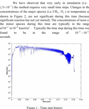
The methane mechanism is solved for species concentration and temperature for nearly 0.164 seconds of physical time. The evolution of the time step is plotted in Figure 1.
We have observed that very early in simulation (i.e. t
≤ ) the method requires very small time steps. Changes in the concentrations of the major species (i.e. ) or temperature as shown in Figure 2, are not significant during this time (because significant reaction has not yet started). The concentrations of most of the minor species during this time are typically in the range of . Typically the time step during this time was found to be in the range of
seconds.
5
5 10× −
4
CH , O2
-17 -10 3
10 to 10 kmol/m
-13 -11
10 −10
Figure 1 : Time step history
A similar behavior was observed when the temperature and concentrations of major product species H2O and CO2 are almost at
equilibrium values (Figure 2). During this time, the small time step is somehow justifiable because some species i.e. CO, CH2O and O2 are
still decaying. Carrying on the simulation for a very long time, such that all species have attained their equilibrium concentrations will result in an increased time step.
We found that this behavior was due to the convergence criteria used for the time step (equation (7)). During the initialisation period the concentration of most of the species (except ) are negligible. In order to avoid numerical errors in the code the minimum concentration is limited to . Because of the small initial concentrations, a small change in concentration will easily violate the convergence criteria. This violation forces the method to take smaller than necessary steps. This behavior will remain until the concentration has reached some larger physical value (i.e. typically )
4 2 2
CH , O , N
-17 3
1×10 kmol/m
-10 3
1×10 kmol/m
To prevent this behavior, a slight modification is proposed in the convergence criteria, by introducing an additional parameter, δ. The criterion takes the following form:
Figure 2 : Temperature and concentrations of different species
( )
c p
i i
c i
y y
y δ ξ
− ≤
+ (13)
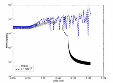
The introduction of δ will increase the denominator of equation (13) to some larger value so that a criterion is not unnecessarily violated. Calculations with the value of δ = ×1 1 0−1 0
were carried out and compared with the results obtained via the original criteria. It is observed that the new technique takes large time steps during the initial integration. Once the concentrations of rapidly growing species (i.e. OH, HO2, CH3) have sufficiently grown
( ), the effect of the new criteria diminishes and the method becomes similar to the original one. The new method has achieves an increased time step of after a few initial steps as shown in Figure 4. The contribution to the computational time saving is mainly achieved during the initial integration (
-10
10
≥ ∼
-7
10
∼
4
10
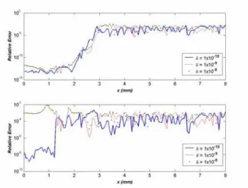
t≤ − ). Due to the comparatively large time steps at the start of the integration, an accuracy loss is expected. The relative mean square (RMS) error analysis of the species concentration plotted in Figure 3 shows that error decreases with the time.
1 2 3
i ,original i , i
i ,original
y y
e i , , ...N
y
δ −
= =
Figure 3: Decrease in RMS error with the simulated time
2
1 N
i i rms
e e
N
=
=
∑
%
%
(15)
The time step response for later integration times is shown in Figure 5 for both criteria. A major portion of time was also saved in this phase. The simulation with both criteria was carried out for 0.164 seconds and an overall time saving by a factor of 15 was achieved.
Figure 4: Time step response with original and modified criteria during pre heat time.
1D-FLAME CALCULATIONS
For this part of the study, individual points within the flame were assumed to provide the initial conditions for homogeneous
α-QSS integration. The individual points were taken from the preheat zone, the reaction zone and equilibrium zone. We are aware that the flame is not a homogeneous structure, nevertheless, by performing a short time integration (t ≤ 10-6), the algorithm should provide an estimate for the allowable time step in that region of the flame.
In the previous section we noted that the difference of results for the original and revised criteria is only visible before 6
1 10× − seconds. This finding is of particular interest because chemically reacting flows are normally solved by process splitting methods [4]. Effects of all physical processes are separately calculated for a chosen global step
(∆tg). The chemical changes are evaluated by integrating the ODEs
over ∆tgusing a stiff integrator. The integration results are provided
to the system, which will combine the effects of all processes. The global step ∆tgis normally much larger as compared to the time step
of the chemical integrator and in all practical cases it will be larger than 6
1 10× − seconds. The requirement of the overall system is that it must have a set of accurate values from all sub processes after each global step irrespective of intermediate calculations.
Figure 5: Time step response with original and modified criteria during post ignition period.
The results obtained with the modified criteria after an elapsed time of 6
1 10× − seconds are found to be in agreement with the original criteria. Comparison of time step, temperature and some species concentrations are carried out in terms of relative error for different values ofδ.
The relative error analysis is carried out using equation (14) and is plotted for different species and temperature (Figures 5 - 8). In almost all cases, the error is found to be 4
1 10
e%≤ × − for 10
1 10
δ= × −
. However, for larger values ofδ, the error increases ( ) in the low temperature region where concentrations of most of the species are low. In contrast, the error is acceptable in the reaction and equilibrium zones. This finding validates the observation that the new approach only relaxes the convergence criteria where the time step is controlled by species having very low concentrations ( ). In regions where major species (or other species having significant concentration i.e. ) are active, the time step is similar to original criteria and hence relative error is also minimal. Selection of the optimum value of
3 1
10− −10−
∼
10
10−
≤ ∼
10
10−
≥ ∼
δ is important to reduce the relative error in the low temperature region. In this case δ =10-10 seems appropriate because in the case of temperature (and many of the minor species) the relative error is small. A guideline for selection of the δ is given at the end of this section.
The relative error in temperature in the pre-heat zone is found to be in range of . However errors in the reaction and equilibration zones are (Figure 6). Figure 8 shows the relative error for CH4 and OH respectively. The error of
CH4 is negligible in the preheat zone because of the fact that the
-17 -8
1×10 to 1×10
6
10−
concentration of CH4 is nearly constant in that region. Relative errors
for H are shown in Figure 9: these are negligible at the start of pre-heat region this is because the concentration of H remains negligible ( 3) in this region.
1×10 -17 kmol/m
Selection ofδ : Selection of this factor is problem dependent. Guidance on its selection can be obtained from two considerations.
(a). Initial concentrations of the species, and the amount of concentration which can be considered insignificant for that specific calculation. In most of cases, values between
to can be considered to have very small effect on overall calculations.
17
1 10× − 13
1 10× −
(b). The size of global step. Very large values of δ will result in a large local step. This may result in a local step larger than the global step.
Typically, values of have been found to give satisfactory results.
10
1 10
δ= × −
Figure 6 Relative Error for temperature profile at diffrent values of δ
Figure 7: Profile of CO2 concentration and relative error.
Figure 8: Relative errors for CH4 and OH
Figure 9: relative error for H and CH3
VI. CONCLUSIONS AND FUTURE WORK
The performance of the α-QSS method for moderately stiff methods is found to be appropriate. The method is not considered an attractive approach for detailed mechanisms due to the small time steps required especially in the pre heat zone. In the pre heat zone the concentrations of the major species are found to be almost constant whereas all other species have negligible concentrations. Unnecessarily small steps in this zone rendered the method inefficient. This inefficiency was identified with the convergence criteria. Commonly available explicit methods are easier to implement and proceed with almost the same time step; hence, it is difficult to say that the QSS method outperforms the explicit methods.
The method can be expected to perform more efficiently by modifying its convergence criteria. We observe a reduction in computational time by a factor of 15 using this modification. The error analysis has shown that the new criterion has produced results with acceptable accuracy. The relative error is found to be 4
1 10
e%≤ × − in
almost all cases. A more extensive criterion for selection of the δremains as future work.
Future research work can be carried out for development of a hybrid numerical scheme, which deals the pre-heat, reaction and equilibration zones separately. An explicit scheme might be employed in the pre-heat and equilibration zones, whereas in the reaction zone (where the system is more stiff) an implicit scheme may be used.
REFERENCES
[1] Viollet, Pierre-Louis, EROFTAC (European Research Community on Flow Turbulence and Combustion) Bulletin 26, 6(1995)
[2] Oijen, J V Flamelet generated Manifolds: Development and application to premixed laminar flames, PhD thesis, Eindhoven university Press, 2002
[3] http://www.visionengineer.com/env/kyoto_agreement.shtml [4] Oran , E S and Boris, J P Numerical Simulation of Reactive
Flow. 2nd Ed, Cambridge university Press, 2000.
[5] Clifford, Milne, Turanyi and Boulton, An Induction parameter Model for shock induced Hydrogen Combustion simulations,
combustion and flame 113, 106 (1998).
[6] Peters, N and Kee R J The computation of stretched laminar methane – air diffusion flames using a reduced four-step mechanism, Combustion and Flame 68, 17(1987)
[7] Peters N. and Williams F.A, Asympototic structure of stoichiometric methane – Air flames, Combustion and flame 68 , 185 (1987)
[8] Lambert, J. D., Numerical Methods for Ordinary Differential
Systems (Wiley), 1991.
[9] D.R. Mott. Ph.D thesis, the university of Michigan, April 1999. [10] Radhakrishnan, K NASA technical paper 3315, 1993.
[11] Mott, D.R., Oran, E.S. and Lee B.V., A Quasi steady state solver for the stiff Ordinary differential equations of reaction kinetics, Journal of Computational physics 164 , 407(2000)
[12] T.R. Young and J.P. Boris, A numerical technique for solving ordinary differential equations associated with the chemical kinetics of reactive-flow problems, Journal of Physical Chemistry. 81, 2424 (1977)
[13] Verwer, J.G and Loon, M Van, An evaluation of explicit Pseudo-steady-state Approximation schemes for stiff ODE system from chemical kinetics, Journal of computational physics 113, 347(1994).
[14] Verwer, J.G and Simpson. Explicit methods for stiff ODEs from atmospheric chemistry, Applied Numerical mathematics 18,
[15]L. O. Jay, A. Sandu, F. A. Potra, G. R. Carmichael, Improved Quasi-Steady-State-Approximation Methods for Atmospheric Chemistry Integration, SIAM Journal of scientific computing 18, 182 (1997)
[16] Kee, R.J, Ruply, F.M. and Miller J.A., The CHEMKIN thermodynamics data base, Sandia National laboratories Report, SAND87-8215B (1997).
[17] Conte, Samuel Daniel , Elementary numerical analysis : an algorithmic approach, McGraw Hill, (196