The dynamics of growth and distribution in a spatially heterogeneous world

The dynamics of growth and distribution

in a spatially heterogeneous world

Paulo Brito

UECE, ISEG, Technical University of Lisbon

2.12.2004

Abstract

This paper tries to reconcile growth and geographical economics by dealing di-rectly with capital accumulation through time and space and by seeing growth conver-gence and spatial agglomeration as jointly generated by dynamic processes displaying pattern formation. It presents a centralized economy in which a Bergson-Samuelson-Millian central planner finds a flow of optimal distributions of consumption, subject to a spatial-temporal capital accumulation budget constraint. The main conclusions are: first, if the behavioral parameters are symmetric, but there is an asymmetric distribu-tion of the capital stock, then the long run asymptotic distribudistribu-tion will be spatially homogeneous; second, if there is homogeneous distribution of the capital stock, but there is an asymmetric shock in any parameter, then the economy will converge towards a spatially heterogeneous asymptotic state; third, spatially heterogeneous asymptotic states will only emerge exogenously, not endogenously; fourth, the spatial propagation mechanism can give birth, when the production function is close to linear, to a Turing instability, which implies that for some parameter values, a conditionally stable space-time distribution should display spatial pattern formation.

Keywords: Optimal growth and distribution; Spatial growth; Optimal control of par-tial differenpar-tial equations; Traveling waves; Fourier transforms; Turing instability. JEL Classification: C6, D9, E1, R1.

∗

Address: ISEG, Rua Miguel Lupi, 20, 1249-078 Lisboa, Portugal. Email: [email protected]. Tel: +(351) 21 3925981. Fax: +(351) 21 3922808.

0

1

Introduction

The interaction between the temporal and the spatial dimensions of capital accumulation,

has been recently readdressed, both theoretically and empirically, by the new (endogenous)

growth and the new geography strands of literature. They tend to reach conflicting

conclu-sions about the dynamics of growth across space.

The existence of convergence towards a long run distribution, displaying a higher degree

of homogeneity across economies, seems to emerge as the consensus view among growth

theorists. This conclusion appears to be fairly robust across different data sets, not only

including countries but also regions within countries. There is empirical evidence of both

β₋ convergence and σ₋ convergence, or, at least, evidence in favor of the existence of an ergodic long run distribution of income across countries (see the surveys by Temple (1999)

or in (Barro and Sala-I-Martin, 2004, ch.11-12)).

However, new economic geography observes that the world economic activity is highly

concentrated in a relatively tiny proportion of the earth’s surface, and that the agglomeration

seem to dominate the dispersive forces. Geographical concentration is observed, not only

for the world economy but also at many several other levels: on metropoli or coasts, within

countries, or on particular locations, for many industries (see Fujita et al. (1999) and Fujita

and Thisse (2002)).

How can we reconcile analytically those two observations ? We explore in this paper

the following answer: First, those disparate conclusions may be related to the structure of

the benchmark models in both areas, in particular to the independence between the spatial

and the temporal dynamics of capital accumulation. Second, if we consider their interaction,

then heterogeneous local growth dynamics, associated to the emergence of pattern formation,

may exist.

The founding papers on the new endogenous growth theory, Romer (1986) and Lucas

(1988), and the voluminous subsequent literature deal mainly with closed economies 1_{. The}

other core assumptions are: utility functions are homogeneous, marginal returns to capital

are decreasing, at the firm level, and there is a mechanism allowing for unbounded growth

(which can be aggregate constant returns to scale and accumulation of human capital or

externalities implying the existence of aggregate increasing returns to scale). Decreasing

marginal returns to capital at the firm level is the main mechanism generating

conver-gence, both within and across different locations. Asymmetry in parameters affecting the

endogenous growth rate explain differences in growth experiences, between different pairs of

countries and locations (absolute or relativeβ₋ convergence).

Included in this strand of literature, there are some recent contributions dealing with

endogenous growth in an open economy context, and with the existence of a (bounded)

world distribution of income. In particular, Acemoglu and Ventura (2002) prove that even

if there are some (mild) increasing returns domestically, the existence of a world capital

market, together with spatial frictions, will produce convergence towards an asymptotic

homogeneous long run world distribution of income. Capital diffusion and the dynamics of

the real exchange rate will tend to equalize real rates of return throughout space, thereby

producing aggregate decreasing returns at the country level.

The new economic geography strand of literature has elected location and agglomeration

as the main subjects of enquiry. Most of the contributions deal with the spatial dynamics

without considering capital accumulation through time. Agglomeration is conceived as a

result of the trade-off between transport costs and increasing returns, within a Dixit-Stiglitz

1

monopolist competition framework (see Fujita et al. (1999) and Fujita and Thisse (2002)).

In general, the only factor that is mobile inter-regionally is labor and capital is immobile.

There is some work addressing endogenous growth and agglomeration in this framework,

where human capital externalities and/or Schumpeterian R&D activities are the engines of

growth, but again, the only mobile factor is labor (see Palivos and Wang (1996), (Fujita and

Thisse, 2002, ch 11) and Martin and Ottaviano (2002)).

Given the spatial-temporal framework which is chosen in both strands of literature, the

mechanisms that generate growth and convergence exclude the existence of agglomeration,

and vice-versa.

This paper tries to reconcile growth and geography by dealing directly with the dynamics

of heterogeneity and by defining variables as jointly dependent on time and a state variable

2_{. Three main assumptions define the setup of this framework.}

The first assumption is related to the features of the support for heterogeneity. We

assume that there is a one-to-one correspondence between heterogeneous (or asymmetric)

agents and their location in a particular point in space. This space has a metric which is

related to economic distance, not geographical distance; we assume that it is one-dimensional

and unbounded and serves as an indexing device as in Hotelling (1929). This choice will

have consequences on the acceptable spatial weighting schemes and on spatial and temporal

boundary conditions.

The second is related to the specification of the spatial-temporal constraints. Though

the equilibrium condition between savings and investment still holds, the intertemporal and

interspatial allocation of capital are mutually consistent. Capital flows among regions is a

function of the spatial gradient of its initial distribution: regions with higher capital intensity

have smaller real rates of return and therefore export capital. Mathematically, a forward

2

parabolic partial differential equation represents the instantaneous budget constraint.

The last assumption is related to the specification of the spatial-temporal arbitrage

condi-tions. We present a centralized economy in which the planner decides on the spatial-temporal

allocation of consumption that maximizes a social welfare Bergson-Samuelson utility

func-tional 3_{. In order to deal with the problems arising from the unbounded support for space,}

we assume a Millian average utility function. A generalized Euler condition is represented

by a backward parabolic partial differential equation.

In addition, the behavioral functions, which characterize the representative agents in

ev-ery point in space, are neo-classical: utility and production functions are concave. Therefore,

we present a generalization of the Ramsey (1928), Cass (1965) and Koopmans (1965) model

for a continuum of open and interacting economies.

There is some literature dealing with a similar economy: Chatterjee (1994), study a

discrete time discrete space economy, Isard and Liossatos (1979), present a continuous-time

continuous and bounded space economy, but do not attempt at solving the model, and

Camacho et al. (2004), which is closely related to our paper, deal extensively, and rigorously,

with existence results for a model with a bounded space and linear utility.

Our model boils down to a particular problem of optimal control of parabolic partial

differential equations, for which we derive heuristically a maximum principle. We also study

qualitatively both the asymptotic distribution and the local stability properties of the optimal

solution. The most surprising feature of the local (distributional) dynamics is the potential

occurrence of total instability, when the related a-spatial Ramsey-Cass-Koopmans model

displays conditional stability. The type of instability is analogous to the Turing (1952) type of

instability. (Fujita et al., 1999, ch. 6) also consider diffusion in a continuous space framework

and report the emergence of spatial heterogeneity, as a result of the existence of Turing

instability. They conclude that spatial interaction among symmetric regions may eventually

3

lead to the emergence of agglomeration, through a mechanism of pattern formation. In our

model, spatial pattern formation may also emerge, for particular values of the parameters.

However, differently from the two previous cases, it may have to characterize the conditionally

(distributionally) stable optimal consumption and capital accumulation trajectories.

Intuitively, the two diffusion mechanisms, related to spatial contact, seem to generate

externality effects, both in consumption and in production that, in some cases, offset the

stabilizing properties of the decreasing marginal productivity of capital. In those cases, a

bounded long run distribution of consumption and capital will only exist if the central planner

limits the workings of the diffusion mechanisms. Therefore, both convergence towards a

asymptotic distribution of capital and agglomeration may occur.

The main conclusions of the paper are the following: first, if there is symmetry in the

behavioral parameters, but an initial non-homogeneous distribution of the capital stock,

then the long run asymptotic distribution will be spatially homogeneous; second, if there

is initially a homogeneous distribution of the capital stock, but there is an asymmetric

shock in any parameter, then the economy will converge towards a spatially heterogeneous

asymptotic state; third, spatially heterogeneous asymptotic states will only emerge as a result

of exogenously determined factors and will not be created endogenously; fourth, the spatial

propagation mechanism can give birth, when the production function is close to linear, to

an analogous of the Turing instability, which implies that for some parameter values, a

conditionally stable space-time distribution will have to display spatial pattern formation.

The rest of the paper is organized as follows: section 2 presents the components of the

model, section 3 presents and derives the optimality conditions according to a generalized

Pontriyagin principle, section 4 uses results on traveling waves’ literature to address the

asymptotic states for the optimal solution, section 5 studies local (distributional) stability by

using Fourier transform methods, section 6 derives the comparative (distributional) dynamics

formulae for productivity shocks and applies them to both symmetric and asymmetric shocks,

2

The model

Let there be a continuum of potentially heterogeneous and interacting households. We will

identify the support of that continuum with space. All the variables are referred to the

time-space coordinates, (t, x) _∈ (X,T) = (R×R+). The reference location, at x = 0, may

be labeled after the location with an initially higher capital intensity4_.

We also assume that population is evenly distributed across space, that there is no

labor migration and that there is only one homogeneous good in the economy. For most of

the paper, spatial heterogeneity refers to differences in the quantities of the good which is

consumed and produced in different locations.

The representative household, in each location, performs production, consumption and

investment activities.

2.1

Households’ problem at location

x

Letc(x, t) be the rate of consumption at timetandC(x)t :={c(x, τ) : t≤τ <+∞}be the path of consumption starting at time t _∈ T, for the representative household located at x. We assume that household preferences are symmetric across space: both the intertemporal

and the instantaneous utility functions and the rate of time preference are identical and

space-independent. The intertemporal utility function, for the household located at x, is assumed to be additively separable and discounted,

V(C(x)0) := Z +∞

0

u(c(x, t))e−δtdt (1)

whereδ >0 is the rate of time preference andu(.) is the instantaneous utility function, which is assumed to be is increasing, concave and Inada: u′_{(.) > 0, u}′′

(.)< 0, limc_→0u(c) = +∞

and limc→+∞u(c) = 0.

4

If one would like to consider jointly heterogeneities related to both to economic distance and geographical distance we could add another dimension, asx_∈R2

In every location, production uses capital and labor with a space-independent

neo-classical technology. We exclude the existence of explicit externalities leading to the existence

of explicit agglomeration effects.

We work directly with per capita variables, by assuming that there is a fixed, constant

and immobile labor supply, L = 1. Let (per capita) production and the stock of physical capital bey(x, t) and k(x, t), at location x at time t, respectively. The production function is y(x, t) = Af(k(x, t)) where f(.) is increasing, concave and Inada: f′_{(.) > 0, f}′′

(.) < 0, limk→0f(k) = +∞ and limk→+∞f(k) = 0. A is an exogenous productivity parameter, not

necessarily space-independent. The marginal productivity, or the real rate of return, of

cap-ital isr(x, t) =Af′

(k(x, t)). The former assumptions exclude the existence of differentiated production technologies across space, implying that differences in the marginal productivity

of capital will only be related to the distribution of the per-capita stock of capital. There is

an inverse relationship between capital intensity and the real interest rate.

Households increase the scale of production by accumulating physical capital. If there

are no (intertemporal) adjustment costs nor depreciation, then gross investment in location

xat time t is ∂k

∂t, and the x-household budget constraint is, for any pair (x, t)∈(X,T),

∂k(x, t)

∂t +c(x, t) +τ(x, t) =Af(k(x, t)),

where τ(x, t) denotes both the households’ excess of production over expenditures and its net lending capacity. The non-Ponzi game condition holds for every point in space, x_∈X,

lim t→∞e

Rt

0r(x,s)dsk(x, t)≥0.

2.2

Regions

Identifying_Rwith the world allows us to identify theσ₋algebra of the Borel sets (_R,_B) with the sets of all regions. Let a particular region,i, be represented byXi = [xi, xi+∆xi]. Assume that the world is composed by the union of all the mutually disjoint regions, _X = S

Preferences, technology and endowments are symmetric and the capital market is perfect

within regions. Therefore, we may consider a single representative agent located in each

region and we may address the interactions among regions as interactions among potentially

asymmetric representative agents.

As the world is a closed economy, meaning that

Z

X

∂k(x, t)

∂t +c(x, t)−Af(k(x, t))

dx=₋

Z

X

τ(x, t)dx= 0 _∀t_∈T,

then, spatial interactions will only take place among regions, if regions are open. When

regions are closed, the aggregate distribution of capital may vary through time. But this will

only occur as a result of independent intertemporal arbitrages within each region. If regions

are open then there will be both (interdependent) intertemporal and interspatial arbitrages.

2.3

Autarkic regions

As a first approximation, assume that all regions are closed: there are no capital flows among

regions. Then, real transfers of goods between regions cannot be financed, and, therefore

trade balances must be instantaneously and permanently cleared, i.e., R

Xiτ(x, t) = 0 for all

(Xi, t) ∈(B,T). Therefore, in an autarkic economy the following regional balance equation should hold

Z

Xi

∂k(x, t)

∂t +c(x, t)−Af(k(x, t))

dx= 0, ∀(Xi, t)∈(B,T).

From now on, let ∆xi → 0 and denote the distribution of consumption and capital, at time t asC(t) := _{c(x, t) : x_∈X} and K(t) :=_{k(x, t) : x_∈X}.

A sufficient condition for regional balance is that

∂k(x, t)

∂t =Af(k(x, t))−c(x, t), ∀(x, t)∈(X,T). (2)

Independently from the existence of a centralized planner, or a distribution of planners for

of a continuum of spatially parameterized Ramsey (1928), Cass (1965), Koopmans (1965)

models, such that given an initial distribution of capital K(0), the representative agent determines an optimal trajectory for consumption ˆC(x)0 and capital accumulation ˆK(x)0 := {k(x, t) :t_∈T} such that it maximizes the intertemporal utility function (1) subject to the budget constraint (2).

Applying the maximum principle to every autarkic location, x, there is a piecewise-continuous function, in time, q(x, t) such that the first order conditions are, given by

u′(c(x, t)) = q(x, t)

dq(x, t)

dt = q(x, t)(δ−r(x, t)) (3) dk(x, t)

dt = Af(k(x, t))−c(x, t) (4)

lim t→∞e

−δt_{q(x, t)k(x, t) = 0.}

The standard neoclassical assumptions on preferences and technology imply that there is

an equilibrium point for every location. If there is symmetry in the parameters, then there

will be an asymptotic homogeneous distribution of c(monotonously related with q) and k, (c, k), which is continuously replicated in time and space. That is,c(x, t) = c, andk(x, t) = k

for every (x, t)∈(X,T), such that δ =Af′(k) = r(k) and c(q) =Af(k).

If there is an initial, non-steady state, asymmetric distribution of capital, K(0)₆=K :=

{k(x, t) =k :∀(x, t)∈(X,T)}, then a distributional dynamics will follow. The evolution of

K(t) will only be generated by intertemporal arbitrage: first consumption will increase for regions in which capital is bellow their steady state level (because in these regions the rate

on return of capital is higher than in the steady state) and net savings will also be positive,

which will imply an increase in the region’s stock of capital.

If, in a neighborhood of the homogeneous steady state, the determinant of jacobian of

equations (3)-(4), is

then there will be conditional saddle-path stability andβ-convergence. As every region dis-plays conditional stability, then the world distribution will also converge to an homogeneous

distribution. If we measure the variance of the world’s distribution of the capital stock by

σ2(t;k) = lim x→∞

1 2x

Z x

−x

(k(x, t)₋E(t;k))2dx

where the average isE(t;k) = limx_{→∞ 2}1_x

Rx

−xk(x, t)dxthen we will also haveσ−convergence asσ(0)> σ(_∞) = 0.

Even in the case in which the steady state distribution is heterogeneous (because there is

asymmetry in any parameter), two conclusions emerge: first, the dynamics of the aggregate

distribution is only determined by the fact that, for each region, the initial capital

endow-ment is different from the steady state capital stock, second, the dynamics of the capital

distribution is independent from any spatial interaction, it will only change as a result of

local intertemporal arbitrage.

2.4

Open regions

When capital and goods flow among regions, then the aggregate balance equation for region

Xi ∈ B now becomes

Z

Xi

∂k(x, t)

∂t +c(x, t) +τ(x, t)−Af(k(x, t))

dx= 0, _∀(Xi, t)∈(B,T),

whereτ(x, t)₆= 0 is the net sales of goods produced in Xi to other regions. In a centralized economy, they will be matched by reallocations of capital among regions. In a decentralized

equilibrium setting, we would assume that there would exist an interspatial capital market

in which stocks would be traded. In the absence of adjustment, transactions or any other

frictional costs, for moving across space, physical capital and its collateral will have the same

value.

opportunities, by flowing from regions with lower marginal productivity of capital towards

regions with higher marginal productivity of capital. As there is symmetry in technology,

and the production function displays diminishing marginal returns to capital, then capital

flows from regions in which it is relatively abundant towards regions in which it is relatively

scarce. If there are no institutional barriers to capital flows, and as regions are internally

homogeneous, then the current account balance for regionXi is measured by the symmetric of the difference of capital intensities with the adjacent regions

Z

Xi

τ(x, t)dx=−

∂k

∂x(xi+ ∆xi, t)− ∂k ∂x(xi, t)

.

As,

∂k

∂x(xi+ ∆xi, t)− ∂k

∂x(xi, t) =

Z xi+∆xi

xi

d dx

∂k ∂x

dx=

Z

Xi

∂2_k

∂x2dx,

then the aggregate budget constraint, for regionXi is given by

Z

Xi

∂k(x, t)

∂t −

∂2_{k(x, t)}

∂x2 +c(x, t)−Af(k((x, t))

dx= 0, ∀(Xi, t)∈(B,T).

If ∆xi → 0, then the instantaneous budget constraint is represented by the quasi-linear parabolic partial differential equation

∂k(x, t)

∂t =

∂2_{k(x, t)}

∂x2 +Af(k(x, t))−c(x, t) ∀(x, t)∈(X,T).. (6)

If thex−household has positive (negative) savings then this will imply both a temporal and a spatial change in the distribution of capital: the household may accumulate (deccumulate)

capital by changing its capital stock, and therefore the level of its future production, and/or

shift capital to other regions (or, in a decentralized setting, sell or buy equities).

The new economic geography theory highlights two main forces that operate through

space: diffusion and agglomeration. Equation (8) presents capital accumulation through

time and diffusion across space 5_{. We will see that, when we consider the joint dynamics of}

5

capital and consumption, agglomeration may emerge from their interplay, as a Turing

insta-bility. This means that by introducing spacial contact and diffusion we may get implicitly

agglomeration dynamics, and do not need to introduce it explicitly6_.

2.5

Efficient consumption distribution

When goods and capital may be freely reallocated among heterogenous agents, we should

have a single central planner that chooses not only the optimal intertemporal allocation of

consumption, but also the optimal intratemporal distribution across different locations. The

optimization criterium should consider not only aggregation of preferences across time but

also across space.

The discounted and additively separable intertemporal utility function (1) presents a

benchmark aggregation for utilities through time for the representative agent located in

each point in space. Even when we consider intertemporally dependent preferences, the

exponential time discounting would still present a natural weighting scheme.

Though we do not intend to dwell into the deep issues related to the definition of a

collective preference relationship, we should observe that the choice of an aggregate utility

function, when there is spatial asymmetry, is not as settled as for the case in which there is

asymmetry. In order to stay close to a Pareto criterium, based upon the maximization of

individual welfare, we will assume a Bergson-Samuelson social welfare function7 _{and extend}

it to an intertemporal context.

Accepting an aggregate criterium, based upon a weighted sum of independent individual

intertemporal utility functions, is only a first step. Next we have to address the problems of

6

Explicit introduction of agglomeration may lead to a highly non-linear structure, that would have con-sequences on the characteristics of the asymptotic distribution of capital.

7

choosing a spatial weighting scheme and of dealing with the unboundedness of the spatial

support.

Benthamian, Millian, von-Neumann-Morgenstern, egalitarian or Rawlsian utility

func-tions 8 _{are based upon different weighting criteria, and verify reasonable ethical postulates.}

A Benthamian utility function would be defined, in our setup, as a simple, unweighted, sum

of the individual intertemporal utility functions, for the representative households located

in every point in space,

Z +∞

−∞

Z ∞

0

u(c(x, t))e−δt_dtdx.

This utility functional solves the aggregation problem but not the unboundedness problem:

the intertemporal aggregate utility will be unbounded, even in the case in which all the

admissible distributions would tend to a spatially homogeneous bounded steady state 9

All the other collective utility functions introduce some type of spatial weighting. The

simpler weighting schemes are based upon spatial discounting or averaging.

Spatial discounting introduces a symmetry between time and space, by penalizing dates

and locations far away from (x, t) = (0,0)10_{. For instance, space could be discounted in an}

exponential way, leading to the utility functional

Z +∞

−∞

Z ∞

0

u(c(x, t))e−(δt+δxx2)_dtdx,

where δw > 0. However, spatial discounting has two unwelcome features: it introduces a preference relation over locations in space, which violates Harsanyis’s symmetry postulate,

and tends to force rejection of an homogeneous spatial distribution as an optimal distribution

in the steady state (even in the case in which the other parameters of the model are spatially

homogeneous).

8

See Atkinson and Stiglitz (1980) for the related static counterpart. 9

This is the spatial counterpart of the unboundedness problem arising in the undiscounted Ramsey intertemporal utility function,R∞

0 u(c(t))dt. 10

Spatial averaging, weights all the locations in space by the inverse of their relative distance

tox = 0. As weights are spatially homogeneous, then there is not an implicit preference of the central planner for any particular location in space. The following Millian intertemporal

utility function may be seen as a collective utility function based upon an averaging criteria

11

V := lim x_→∞

1 2x

Z x

−x

Z ∞

0

u(c(y, t))e−δt_dtdy.

This utility functional will be bounded for steady state spatially symmetric distributions of

consumption, i.e.,V = u(_δc), allowing for the comparison of alternative optimal distributional strategies. We will assume a Millian central planner from now on.

2.6

Boundary conditions

The solutions of partial differential equations depend on the specification of the boundary

conditions. Three types of alternative boundary conditions can be found in the applied

mathematics literature and be adapted to our model: free boundaries if limx_→±∞k(x, t) and limx→±∞ ∂k∂x(x,t) are not specified, or Cauchy or Dirichlet boundaries if limx→+∞k(x, t) = k(t) and limx_→−∞k(x, t) = k(t) or if limx_→+∞∂k∂x(x,t) =

∂k

∂x(t) and limx→−∞ ∂k(x,t)

∂x =

∂k

∂x(t) were given, respectively. Neumann (or no-flux) boundaries limx→+∞∂k∂x(x,t) = limx→−∞

∂k(x,t)

∂x = 0

are a popular special case.

The choice of the particular boundary condition depends on the type of heterogeneity,

that we are considering. As, in our case,xis close to spatial location, the choice of the central place is arbitrary. A boundary condition that ties down the stock of capital of distant regions,

would introduce incentives for the dispersion of capital and would imply that the choice of

the optimal distribution of consumption would be determined exogenously. As our focus is

related with the general properties of the dynamics of the capital distribution, it is irrelevant

which geographical regions lay at a particular point in the distribution along time. Then

11

Cauchy boundaries would be inappropriate.

Neumann boundaries would be a candidate for a state-space as X = [0,+_∞), where

x = 0 could stand for the richest region and x = +∞ for the poorest. The existence of a smooth distribution function would be possible if we would assume, tautologically, that

capital could not move outside those boundaries. Neumann boundaries would allow for more

flexibility than the Cauchy boundaries, because they would not eliminate the limit situation

of homogeneity. However, from the application of Pontriyagin’s maximum principle, the

central planner would have a very strong incentive to allocate consumption to the extremes

of the distribution. The dual boundary conditions would be limk_→±∞ ∂c_∂x(x,t) = +∞. We will assume, instead, the following boundary conditions,

lim x_→±∞

k(x, t)

x = 0, ∀t∈T.,

which is both weaker than the Neumann boundaries and is more realistic. It has the following

property: the ”tails” of the capital stock distribution are bounded functions of time and may

be approximated by constant functions of space.

3

The optimal distributed growth dynamics

The central planner’s problem is built by assembling the elements of the model presented in

the last section. It consists in determining an optimal distributive strategies for consumption

and capital, C∗ _{:= {c}∗_{(x, t) : (x, t) ∈ X × T} and K}∗ _{:= {k}∗_{(x, t) : (x, t) ∈ X × T},}

respectively, such that

V := max

{c(x,t):(x,t)∈(X,T)}xlim→∞

1 2x

Z x

−x

Z ∞

0

u(c(y, t))e−δt_{dtdy. (7)}

subject to

∂k(x, t)

∂t =

∂2_{k(x, t)}

∂x2 +Af(k(x, t))−c(x, t) ∀(x, t)∈(X,T), (8)

lim t→∞e

−Rt

lim x_→∓∞

k(x, t)

x = 0, ∀t∈T (10)

k(x,0) = k0(x), ∀x∈X given. (11)

The next proposition, assumes that an optimal solution exists, and presents an heuristic

version of the necessary conditions according to the Pontryagin’s maximum principle 12_.

Proposition 1. Let (C∗_{, K}∗_{) be a solution of the centralized problem (7)-(11). Then there}

is a flow of distributions, Q := {q(x, t) : (x, t) ∈ X×T}, where q(x, t) is continuous in X

and piecewise continuous in T, such that the solution verifies equations (8), (9), (10), (11) and

u′(c∗(x, t)) = q(x, t), ∀(x, t)∈(X,T) (12)

∂q(x, t)

∂t = −

∂2_{q(x, t)}

∂x2 +q(x, t) (δ−A(x)f

′_(k∗_{(x, t))) ∀(x, t)∈(X,T) (13)}

0 = lim t_→+∞xlim_→∞

1 2x

Z x

−x

e−δt_{q(y, t)k(y, t)dy, (14)}

0 = lim x_→±∞

e−δt_{q(x, t)}

x . ∀t∈T (15)

The planar system of partial parabolic equations, (8)-(13), together with the space-time

limit conditions (10), (11), (14) and (15) and the optimality condition (12) present a direct

generalization of the standard Ramsey-Cass-Koopmans model, for an optimal distribution

policy.

Given an initial distribution of the stock of capital,K(0), as in equation (11), an admis-sible solution should verify the open-economy budget constraint (8), for every date-location

pair, the non-Ponzi game condition (9), as a terminal time constraint for every point in space,

and the boundary conditions (10) for the ”tails” of the distribution of capital in space, for

every moment in time.

An optimal solution is an admissible solution that, in addition, has the following

proper-ties. First, a static arbitrage condition, given by equation (12), holds. It equates the measure

12

of the marginal value of capital, represented by the co-state variable,q(.), with the marginal utility of consumption. For any moment in time, and between any pair of locations, the

ratios in q are directly related to the ratios in the true cost-of-living index, and inversely related to the ratios of consumption. Therefore, if we interpret q as a real exchange rate, locations in which consumption rises should face a real depreciation.

Second, an intertemporal-spatial arbitrage condition, given by equation (13), will also

hold: for every date-location pair, the rate of return on capital should be equal to the rate of

time preference. The rate of return on capital is equal to the sum of the real rate of interest

with the change in value of the stock of capital, resulting from capital accumulation through

time and space. In a decentralized economy setting, the temporal marginal income will be

equal to the change in the value of capital resulting from the investment in one extra unit of

equity, issued in the own region, and the spatial marginal income will be equal to the change

in income obtained from investing in equities issued by neighboring locations. If we use the

real exchange rate interpretation, then equation (13) states an arbitrage relationship between

the rate of time preference and the sum of the rate of return on domestic assets plus the

instantaneous rate of change in the real exchange rate (real appreciation) with neighboring

locations.

Third, a generalized transversality condition, (14), should also be met: the asymptotic

average value of capital should be dominated by an exponential discount factor, where the

rate of time preference is the discount rate.

At last, equation (15) presents a dual counterpart of the boundary condition (10): the

discounted shadow value of capital in the boundaries of the state space, should be close to

constant.

Two spatial diffusive forces are at work in our model. The first is related to the incentives

which drive the redistribution of consumption, seeking to equalize the marginal productivity

of capital with the rate of time preference through space and time. The second is related

diffusive force, the first acts as a backward diffusive force. That is, if at a particular

time-space location there is an expectation that the rate of time preference is higher than the

marginal productivity of capital in any point in the future, which means that there is too

much capital, then consumption will not only increase in that location, but it also increases

more than in neighboring locations. There are, immediately, net imports of goods from

neighboring regions. If we consider the two effects together, then the increase in consumption

will imply both a reduction in net investment, in the own location, and in the investment in

assets on firms located in other regions. In the non-spatial Ramsey model, the decreasing

returns to capital act as a dampening force which generates conditional stability. In our

case, as we will see, the presence of both diffusion mechanisms generate instability, which

may more than offset the stabilizing effect of the decreasing returns.

Next, we will characterize the solutions of the system (8)-(13) by using qualitative

meth-ods13_{. First, we will address the existence, uniqueness and characterization of an asymptotic}

state, and, next, we will study the local dynamics associated to changes in productivity.

4

Asymptotic states

An (optimal) asymptotic state is defined by the distributions of the dual price and of capital, ˜

Q:=_{q(x), x_∈X} and ˜K :=_{k(x), x_∈X}, respectively, that solve the system of ordinary differential equations on space,

∂2_q(x)

∂x2 = q(x)(δ−Af

′_{(k(x))), (16)}

∂2_k(x)

∂x2 = −Af(k(x))) +c(q(x)), (17)

given the boundary conditions (10).

13

The main issue to address is related to the existence of a spatially heterogeneous

asymp-totic state, i.e., to the existence of particular solutions to the system (16)-(17) which vary

with the independent variable. As the behavioral functions are defined implicitly, we may

only supply a qualitative answer.

Heterogeneous asymptotic states may occur exogenously or endogenously. If any

param-eter is spatially dependent, v.g., A =A(x), then the system becomes non-autonomous and the solution will be space dependent. In this case we say that a spatially heterogeneous

asymptotic state is generated exogenously. If all the parameters are homogenous across

space, then two types of solutions may be obtained: a constant or a spatially variable

so-lution. In the first case we will have a spatially homogeneous asymptotic state, and, in the

second, an endogenously generated heterogeneous asymptotic state.

The traveling wave literature (see Volpert et al. (1994)) offers some useful results to

tackle this issue. Traveling waves are solutions of the system (8)-(13) such that the unknown

functions,q(.) andk(.), can be written asq(x, t) = y(ξ) andk(x, t) =w(ξ) where ξ:=x₋ηt. The constant speed of wave propagation is denoted by η. The solutions of system (16)-(17) are a particular case forη = 0.

Let y1(ξ) = dy_dξ(ξ) and w1(ξ) = dw_dξ(ξ), then the PDE system (8)-(13) is equivalent to the

following four dimensional ODE system

˙

y(ξ) = y1(ξ) (18)

˙

y1(ξ) = ηy1(ξ) +y(ξ) (δ−Af′(w(ξ))) (19)

˙

w(ξ) = w1(ξ) (20)

˙

w1(ξ) = −ηw1(ξ)−Af(w(ξ)) +c(y(ξ)). (21)

Again, two types of stationary solutions may exist:

The second case may occur because the equilibrium point of the system (18)-(21) is

unique and if an homoclinic orbit, such that limξ±∞z(ξ) = z, for z := (y, y1, w, w1), exists.

Observe that if it exists for η = 0 then system (16)-(17) will have an homoclinic orbit as well, and its existence is completely consistent with the boundary conditions (10).

Proposition 2. Let η = 0 and let the other parameters be constant. Then the only asymp-totic equilibrium point is the homogeneous distribution.

This proposition is an implication of the fact that there is not enough curvature in

the production function for allowing to the existence of endogenously generated asymptotic

heterogeneous distributions of capital and consumption 14_.

Summing up, we will only have a spatially heterogeneous asymptotic state if at least one

parameter is spatially asymmetric. When the parameters are spatially symmetric, then the

only asymptotic state for the system (8)-(13) is the Ramsey-Cass-Koopmans equilibrium,

replicated across space, K = {k(x) = k : δ = Af′(k), ∀x ∈ X}, and Q = {q(x) = q :

c(q) = Af(k), _∀x_∈X}. Given the neo-classical assumptions on preferences and technology, that spatially homogeneous steady state will exist and be unique, for any point in space.

5

Local dynamics in the neighborhood of an

homoge-neous asymptotic state

A solution to the optimal distribution problem exists if, for any given initial distribution of

capital,K(0), not necessarily spatially homogeneous, there is an initial distribution of prices,

Q(0), (or a monotonously initial distribution of consumption, C(0)) and flow distributions through time,Q(t) andK(t), fort >0, that will converge to a spatially homogeneous steady state, limt_→∞Q(t) =Q, limt_→∞K(t) = K.

Any unbounded trajectory violates both the boundary and the transversality conditions.

As the forward-backward system of partial differential equations has not an explicit solution,

14

we will have to rely again on qualitative methods in order to determine the existence and

characterize the (generalized) stable manifold based upon linearization 15_.

5.1

Linearization

Let uq(x, t) := q(x, t)−q and uk(x, t) := k(x, t)−k denote the space-time local variations of the marginal utility of consumption and of the capital stock, in the neighborhood of a

spatially homogeneous asymptotic state. Assume that at time t = 0 the deviation from the steady state is given by (uq(x,0), uk(x,0)) 6= (0,0), for any x ∈ X. If the integrability and regularity conditions are fulfilled, then the local modified hamiltonian PDE system

(8)-(13), can be approximated, by a system of two homogeneous semi-linear parabolic PDE’s,

∀(x, t)_∈(_X×R++),

∂uq(x, t)

∂t = − ∂2_u

q(x, t)

∂x2 −qAf

′′

(k)uk(x, t), (22)

∂uk(x, t)

∂t = ∂2_u

k(x, t)

∂x2 −c′(q)uq(x, t) +δuk(x, t). (23)

As the spatial support is unbounded, −∞ < x < +∞, a Fourier transformation may be applied16 _as

uj(x, t) =

Z +∞

−∞ U

j(υ, t)eiυxdυ, j =q, k, ∀(x, t)∈(X×R+)

wherei=√₋1 and υ _∈Υ =R and

Uj(υ, t) = 1 2π

Z +∞

−∞

uj(x, t)e−iυxdx, j =q, k, ∀(υ, t)∈(Υ×R+).

That transformation changes the functional dependence of the variables from space, x, to frequencyυ, which represents the speed of spatial propagation of any shock located atx= 0. This new representation has important analytical consequences. By using the properties of

15

We will mainly develop a heuristic approach. See Henry (1981) and Evans (1998) for a rigorous approach on the existence of solutions. See (Smoller, 1994, ch. 11) on the linearization of parabolic PDE’s.

16

the Fourier transforms, then system (22)-(23) becomes

0 =

Z +∞

−∞

∂_Uq(υ, t)

∂t + (iυ)

2

Uq(υ, t) +qAf ′′

(k)_Uk(υ, t)

eiυx_dυ,

0 =

Z +∞

−∞

∂Uk(υ, t)

∂t −(iυ)

2_U

k(υ, t) +c′(q)Uq(υ, t)−δUk(υ, t)

eiυxdυ.

A sufficient condition for the annihilation of the integrals is that integrand be equal to

zero. Then an equivalent spectral representation of (22)-(23) is the linear planar ODE,

parameterized byυ,

∂Uq(υ, t)

∂t = υ

2

Uq(υ, t)−qAf ′′

(k)_Uk(υ, t), (24)

∂Uk(υ, t)

∂t = −c

′_(q)U

q(υ, t) + (δ−υ2)Uk(υ, t), (25)

∀(υ, t) _∈ (Υ_{× R}++), given Uq(υ,0) and Uk(υ,0), at t = 0. This system can be solved explicitly and its solution gives the local dynamics, through time, associated with every

spatial frequency.

5.2

Local conditional spectral stability and Turing instability

Recall, from equation (5), that D < 0 as an implication of the concavity of the production and utility functions. Additionally, let

Υs =

 



R if δ

2 2

+D <0 (_−∞, υ1)∪(υ2, υ3)∪(υ4,+∞) if δ₂

2

+D >0,

where,υ1 < υ2 <0< υ3 < υ4, because

υ1,2 = −   δ 2 ± " δ 2 2 +D # 1 2   1 2 <0

υ3,4 =   δ 2 ∓ " δ 2 2 +D # 1 2   1 2

>0.

We say that there is conditional spectral stability if the trajectory associated with any

Lemma 2. If υ ∈Υs then there is conditional spectral stability.

Therefore two cases may occur: if δ

2 2

+D < 0 then there is conditional spectral stability for any frequency of spatial propagation; but, if δ

2 2

+D > 0 then there will only be conditional spectral stability for some frequencies17_.

A similar result occurs in the presence of theTuring instability, which may exist in planar

forward parabolic partial differential equations. In those equations, Turing (1952) observed

that the diffusive terms may reduce the dimension of the stable manifold associated to the

kinetic part, for some parameter values. In initial value well posed problems, associated

to forward equations, it implies the emergence of pattern formation, i.e., emergence of a

non-homogenous asymptotic distributions. In our case, we have a mixed initial-terminal

condition in time, associated to a system composed by a forward and a backward parabolic

partial differential equation. Then, a transient pattern formation results, for the case in

which δ

2 2

+D >0, when we are forced to eliminate the frequencies associated with total instability, in order to get a non-empty stable manifold18_.

Formally, the conditions enabling the case δ

2 2

+D >0 are the following:

Lemma 3. The likely occurrence of a Turing instability is higher when the rate of time pref-erence and the concavity of the utility function are higher and the concavity of the production function is lower.

5.3

The tangent to the generalized local stable manifold

Proposition 3. Assume that the system is at a given initial distribution K(0) ₆=K, at time

t= 0, and let

λs =

 



δ

2−

"

υ2₋ δ

2

2 −D

#12

:υ _∈Υs

 



<0. (26)

17

There will be mode interaction, associated to a fold bifurcation, if δ

2 2

+D= 0. See Mei (2000). 18

This solution is stronger than necessary. As the transversality condition is computed as an average and as the sum of the eigenvalues is independent from frequencies, becauseλu+λs=δ, if we could compute an

Then, the solutions along the stable space, which is tangent to the stable manifold, are

˜

uq(x, t) =

Z +∞

−∞

hs(w)˜uk(x−w, t)dw, (27)

˜

uk(x, t) =

Z +∞

−∞

uk(z,0)φ(x−z, t)dz, , (28)

for any pair (x, t)_∈(_X,_R++), where the Green’s function for the stock of capital is

φ(y, t) = 1 2π

Z

Υs

eλs(υ)t+iυy_{dυ, ∀(y, t)∈(}

X,R++), (29)

and the slope of the tangent to the stable manifold in the (q, k)-space is

hs(y) = 1 2π

Z

Υs

λu(υ)−υ2

c′

(q) e iυy

dυ, ∀y∈X. (30)

The economy will conditionally converge to a spatially homogeneous steady state (Q, K), through a time-varying distribution which is tangent to (27)-(28). Though there is not an

explicit expression for the integrals, it is easy to see that

lim

t_→∞u˜q(x, t) = limt_→∞u˜k(x, t) = 0, ∀x∈X and

lim

t↓0 u˜q(x, t)6=uq(x,0) limt↓0 u˜k(x, t) =uk(x,0), ∀x∈X.

This result generalizes the well know result for the ”jump” to the saddle manifold in the

Ramsey-Cass-Koopmans model, to the distributional ”jump” ˜uq(x,0)−uq(x,0).

When we have both intertemporal and inter-spatial arbitrage mechanisms, their

interac-tion gives birth to an analogous to Turing instability, which is not present in the homogenous

agent model. In deriving the spectral conditional stability and the related (tangent to the)

stable manifold, we have to eliminate that source of instability. The intuition is the

fol-lowing: if the economy is not in an initial homogeneous asymptotic state, and the spatial

particular generalized saddle path is followed, and the economy will converge to a spatially

homogeneous and bounded asymptotic state. If δ

2 2

−c′

(q)qAf′′

(k) < 0 then the optimal consumption-investment policy will generate a spatially monotonous distribution

realloca-tion of consumprealloca-tion and capital. However, if the δ

2 2

−c′

(q)qAf′′

(k) >0 then the spatial reallocation of capital and consumption will tend to generate an unbounded asymptotic

dis-tribution if that reallocation does not ”discriminate” against particular locations. That is,

the optimal consumption and investment strategies may have to be non-monotonous across

space 19_{. Quah (2002) also found, in a spatial aggregation model, that some sinusoidal}

components have to be omitted for the existence of convergence to a uniform steady-state

equilibrium. Looking at the expression for λs, in equation (26), it appears that the effect of some medium-ranged spatial frequencies has to be eliminated. The explanation seems to be

the following: while the low frequencies tend to counter the effect of the decreasing marginal

productivity of capital, which will work for instability, they seem to inhibit the destabilizing

effect of the spatial re-distribution of consumption by the planner.

Even if we assume concave utility and production functions, as in the

Ramsey-Cass-Koopmans model, the spatial propagation mechanism may originate instability by the way

of an implicit externality. Therefore, spatial agglomeration is a property of the optimal

spatial capital allocation policy in the presence of a potential Turing instability. According

to lemma 3, an optimal agglomeration policy is likelier if the production function is close to

linear and the degree of relative risk aversion is high. This means that both spatial differences

among real interest rates and changes in the real exchange rates are not high. In this case,

there is a complementarity between stronger intertemporal mechanisms (as opposed to

inter-spatial) and the externality effects generated by diffusion. The optimal solution will only

verify the transversality condition if the working of that externality is hampered by the

presence of spatial agglomeration.

19

5.4

Numerical illustrations

To illustrate the results in Lemma 3 and Proposition 3, consider the examples in table 1.

Both assume an isoelastic utility function,u(c) = c1₋θ

1−θ, where θ > 0, and a Cobb-Douglas production function, y = Akα_{, where 0 < α < 1. The two sets of parameters are chosen} in order to allow for δ

2 2

+D < 0, in case 1, and δ

2 2

+D > 0, in case 2. As D =

−c

θα(α−1)k α₋2

, then case 2 occurs for higher δ and θ are an α close to one, as stated in Lemma 3. We consider a slightly more general case with capital depreciation at a constant

rate ρ.

Table 1: Numerical examples case δ α θ ρ A a12 a21 δ₂

2

+D b1,A b2,A 1 0.03 0.3 0.5 0.1 0.704 0.051 1.431 -0.073 -0.207 1.421 2 0.2 0.9 5 0.1 0.357 0.046 0.052 0.008 -2.563 2.799

We also assume, in both cases, that there is an initial asymmetric deviation from a

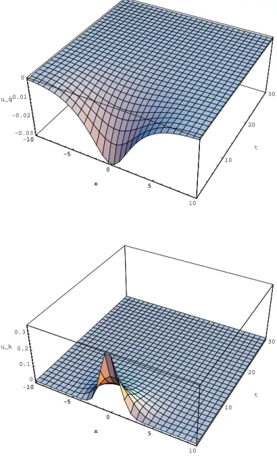
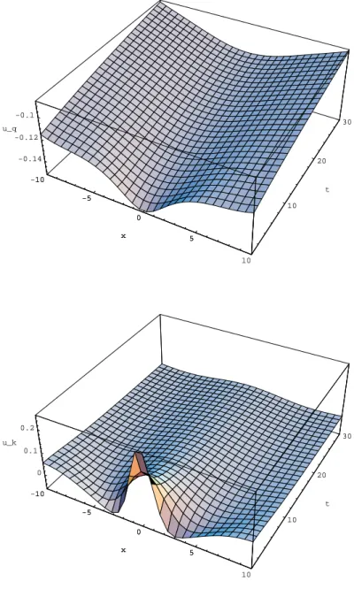
homoge-neous steady state, given by uk(x,0) ∼ N(0,1). Figures 1 and 2 present the space tangent to the saddle manifold for case 1 and case 2, respectively. We observe that the qualitative

dynamics is similar, in both cases. Initially, the locations with more initial capital have lower

relative prices. Therefore, they have higher consumption and a depreciated real exchange

rate. When time passes, those regions export capital and face a process of real appreciation

towards a long run homogeneous distribution of (optimal) capital, prices and consumption.

This positive correlation between the increase in capital endowments real depreciation is

consistent with the findings of Acemoglu and Ventura (2002), who models a world with

imperfectly substitutable goods.

space in case 2. This is, again, a consequence of the effects of the potential Turing instability

and of the their elimination through a transient pattern formation.

6

Comparative distributional dynamics

In the last section we considered an initial heterogeneous distribution, K(0), and symmet-ric parameters. Now, we will assume that the economy is at a stationary homogeneous

distribution, (Q, K), and that there is a, possibly asymmetric, productivity shock dA(x). The next proposition presents comparative dynamics formulae.

Proposition 4. Assume that υ _∈ Υs and that there is a permanent time-invariant and

possibly spatially asymmetric productivity shock, dA(x). Then the short run multipliers, along the saddle manifold are given by equations

uq,A(x, t) = uq,A(x)−

Z +∞

−∞

uk,A(w)

Z +∞

−∞

hs(y)φ(x−y−w, t)dydw, (31)

uk,A(x, t) = uk,A(x)−

Z +∞

−∞

uk,A(z)φ(x−z, t)dz, (32)

for(x, t)∈(X,R++), where φ(.) andhs(.) are given in equations (29) and (30), respectively,

and the asymptotic multipliers are

uq,A(x) =

Z

Υs

Uq,A(υ)eiυxdυ (33)

uk,A(x) =

Z

Υs

Uk,A(υ)eiυxdυ, (34)

where

Uq,A(υ) =

(δ₋υ2_)B

1,A(υ) +qAf ′′

(k)_B2,A(υ)

υ2_(δ−υ2_{) +D} (35)

Uk,A(υ) =

c′(q)B1,A(υ) +υ2B2,A(υ)

υ2_(δ−υ2_{) +D} . (36)

and

B1,A(υ) = − 1 2π

Z +∞

−∞

qf′(k)dA(x)e−iυx_{dx (37)}

B2,A(υ) = 1 2π

Z +∞

−∞

Figure 1: Local stable manifold: case 1

-10

-5

0

5

10 x

10 20

30

t 0

0.1 0.2 0.3

u_k

-10

-5

0

5 x

-10

-5

0

5

10 x

10 20

30

t -0.03

-0.02 -0.01

0

u_q

-10

-5

0

Figure 2: Local stable manifold: case 2, transient spatial pattern formation

-10

-5

0

5

10 x

10 20

30

t 0

0.1 0.2 u_k

-10

-5

0

5 x

-10

-5

0

5

10 x

10 20

30

t -0.14

-0.12 -0.1 u_q

-10

-5

0

Now, on impact, the changes in both variables are limt_↓0u˜q,A(x,0)6= 0 and limt_↓0u˜k,A(x,0) = 0, for anyx_∈X.

Next, we determine the long run multipliers for two particular cases: for a symmetric

shock and for an asymmetric shock in locationx= 0.

Corollary 1. Assume that there is a symmetric, constant, and permanent unit shock,

dA(x) =dA= 1 for any x∈X. Then, the long run multipliers are also symmetric,

uq,A =

(f′(k))2−f(k)f′′(k)

c′

(q)f′′

(k) <0, ∀x∈X

uk,A = −

f′

(k)

Af′′

(k) >0, ∀x∈X.

where (q, k) are the space-wise pre-shock values.

Corollary 2. Assume that there is a Dirac’s delta permanent productivity shock at location

x= 0, i.e., dA(x) =δ(x). Then the asymptotic multipliers are asymmetric across space,

uq,A(x) =

Z

Υs

q

2π

Af(k)f′′(k)−(δ−υ2_)f′

(k)

υ2_(δ−υ2_{) +D}

eiυxdυ

uk,A(x) = − 1 2π

Z

Υs

c′

(q)qf′

(k) +υ2_f(k)

υ2_(δ−υ2_{) +D}

eiυxdυ

where (q, k) are the space-wise pre-shock values.

Given an initial symmetric state, a symmetric shock will generate an asymptotic

sym-metric shift in the capital stock and an asymsym-metric shock will generate an asymsym-metric one.

Also, the long run multipliers are formally the same, independently of the structure of Υs.

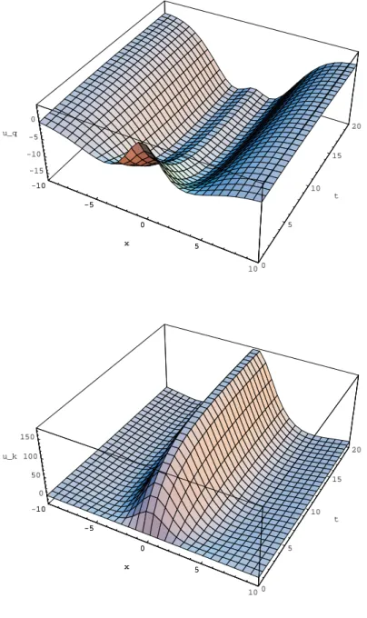
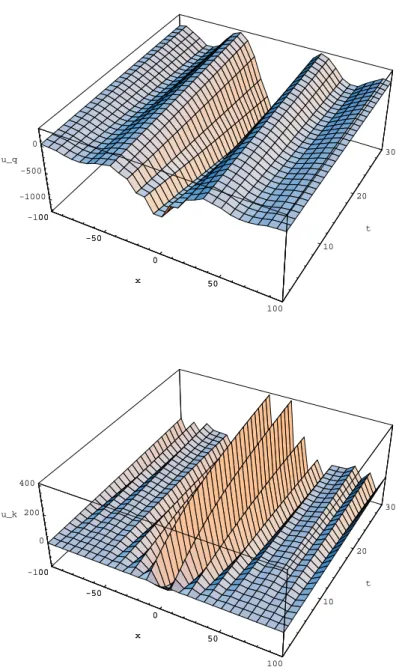
We get a geometrical representation by going back to the examples presented in the last

section and introducing a permanent asymmetric productivity shock dA(x) _∼ N(0_A0,1) _×100 (see Figures 3 and 4). This case is a weighted sum of the Dirac’s delta shocks dealt in

Corollary 2.

They show, firstly, that there is both a short run and a long run increase in the

Figure 3: Dynamics for a shock inA, percentage changes: case 1

-10

-5

0

5

10 x

0 5

10 15

20

t 0

50 100 150

u_k

-10

-5

0

5 x

-10

-5

0

5

10 x

0 5

10 15

20

t -15

-10 -5

0 u_q

-10

-5

0

Figure 4: Dynamics for a shock in A: case 2, spatial pattern formation

-100

-50

0

50

100 x

10 20

30

t 0

200 400

u_k

-100

-50

0

50 x

-100

-50

0

50

100 x

10 20

30

t -1000

-500 0 u_q

-100

-50

0

depreciation affecting the locations that benefit from the shock. Secondly, some partial

spillovers to neighboring locations occur, although the optimal growth and distribution of

consumption will be achieved by keeping capital concentrated in the locations in which it is

more productive. We have relative β-convergence but possibly not σ-convergence. At last, in case 2, the optimal distributive policy is clearly non-monotonous across space and there

will be a clear local pattern formation: for a shock that varies monotonously across space,

there will be long run local agglomerations in the distribution of capital. In this case, the

pattern formation has both a transient and a long run nature.

7

Final remarks

This paper presented an attempt at integrating both spatial and temporal dynamics, by

dealing directly with distributions and with the dynamics of distributions. The main

exten-sions and questions worth addressing with our framework are the following, in our opinion.

First, under which conditions can we get an endogenous long run distribution of capital, v.g.

consistent with Quah (1996) bi-modal distribution of per capita income: will explicit

agglom-eration mechanisms do the job ? Second, the Turing instability may supply another avenue

for generating endogenous unbounded growth: will spatial spillovers generate unbounded

growth even when there are locally decreasing returns to capital ? At last, in modeling a

decentralized economy: is there a structure of markets and institutions which would generate

an equilibrium equivalent, in a Pareto sense, to the solutions of our model ?

References

Acemoglu, D. and J. Ventura (2002): “The World Income Distribution,” Quarterly

Journal of Economics, 117, 659–694.

Barro, R. J. and X. Sala-I-Martin(2004): Economic Growth, MIT Press, 2nd ed.

Beckmann, M. J. (1970): “The analysis of spatial diffusion processes,” Papers of the

Regional Science Association, 25, 109–17.

Bergson, A. (1938): “A Reformulation of Certain Aspects of Welfare Economics,”

Quar-terly Journal of Economics, 52, 310–334.

Bond, E. W., P. Wang, and C. K. Yip (1996): “A general two-sector model of

en-dogenous growth with human and physical capital: balanced growth and transitional

dynamics,” Journal of Economic Theory, 68, 149–73.

Butkovskiy, G.(1969): Distributed Control Systems, New-York: American Elsevier.

Caball`e, J. and M. Santos (1993): “On endogenous growth with physical and human

capital,” Journal of Political Economy, 101, 1042–67.

Camacho, C., B. Zou, and R. Boucekkine(2004): “Bridging the Gap Between Growth

Theory and the New Economic Geography: The Spatial Ramsey Model,” .

Carlson, D. A., A. B. Haurie, and A. Leizarowitz(1991): Infinite Horizon Optimal

Control, Springer-Verlag, 2nd ed.

Cass, D. (1965): “Optimum growth in an aggregative model of capital accumulation,”

Review of Economic Studies, 32, 233–40.

Chatterjee, S.(1994): “Transitional Dynamics and the Distribution of Wealth in a

Neo-classical Model,” Journal of Public Economics, 54, 97–119.

Derzko, N. A., S. P. Sethi, and G. L. Thompson (1984): “Necessary and sufficient

conditions for optimal control of quasilinear partial differential equations systems,”Journal

Evans, L. C. (1998): Partial Differential Equations, vol. 19 of Graduate Series in

Mathe-matics, Providence, Rhode Island: American Mathematical Society.

Fujita, M., P. Krugman, and A. Venables (1999): The Spatial Economy. Cities,

Regions and International Trade, MIT Press.

Fujita, M. and J.-F. Thisse(2002): Economics of Agglomeration, Cambridge.

Harsanyi, J. C.(1955): “Cardinal Welfare, Individualistic Ethics, and Interpersonal

Com-parisons of Utility,” Journal of Political Economy, 63, 309–321.

Henry, D. (1981): Geometric Theory of Semilinear Parabolc Equations, Lecture Notes in

Mathematics, Springer.

Hotelling, H.(1929): “Stability in Competition,” Economic Journal, 39, 41–57.

Isard, W. and P. Liossatos (1979): Spatial Dynamics and Optimal Space-Time

Devel-opment, North-Holland.

Koopmans, T.(1965): “On the concept of optimal economic growth,” inThe Econometric

Approach to Development Planning, Pontificiae Acad. Sci., North-Holland.

Kuznetsov, Y. A.(1998): Elements of Applied Bifurcation Theory, Springer, second ed.

Lions, J. L.(1971): Optimal Control of Systems Governed by Partial Differential Equations,

New-York: Springer-verlag.

Lucas, R. (1988): “On the mechanics of economic development,” Journal of Monetary

Economics, 22, 3–42.

Martin, P. and G. I. P. Ottaviano(2002): “Growth and Agglomeration,”International

Mei, Z.(2000): Numerical Bifurcation Analysis for Reaction-Diffusion Equations, Springer

Series in Computational Mathematics, Springer.

Mossay, P.(2003): “Increasing Returns and Heterogeneity in a Spatial Economy,”Regional

Science and Urban Economics, 33, 419–444.

Mueller, D. C.(2003): Public Choice III, Cambridge.

Neittaanmaki, P. and D. Tiba(1994): Optimal Control of Nonlinear Parabolic Systems,

Marcel Dekker.

Palivos, P. and P. Wang(1996): “Spatial agglomeration and endogenous growth,”

Re-gional Science and Urban Economics, 26, 645–70.

Quah, D. (1996): “Twin peaks: growth and convergence in models of distribution

dynam-ics,” The Economic Journal, 106, 1045–55.

——— (2002): “Spatial Agglomeration Dynamics,”American Economic Review Papers and

Proceedings, 92, 247–52.

Ramsey, F.(1928): “A mathematical theory of saving,” Economic Journal, 38, 543–59.

Rebelo, S. (1991): “Long run policy analysis and long run growth,” Journal of Political

Economy, 99, 500–21.

Robert E. Lucas, J. and E. Rossi-Hansberg (2002): “On the Internal Structure of

Cities,” Econometrica, 70, 1445–1476.

Romer, P.(1986): “Increasing Returns and Long-Run Growth,” Journal of Political

Econ-omy, 94, 1002–37.

——— (1990): “Endogenous Technological Change,”Journal of Political Economy, 98, S71–

Samuelson, P. (1947): Foundations of Economic Analysis, vol. 80 of Harvard Economic

Studies, Harvard University Press, 1965, Atheneum.

Smoller, J. (1994): Shock Waves and Rection-Diffusion Equations, vol. 258 of

Grundle-heren Series, Springer-Verlag, 2nd ed.

Temple, J. (1999): “The New Growth Evidence,” Journal of Economic Literature, 37,

112–56.

Turing, A. M.(1952): “The Chemical Basis of Morphogenesis,”Philosophical Transactions

of the Royal Society of London, series B, 237, 37–72.

Volpert, A., V. Volpert, and V. Volpert (1994): Traveling Wave Solutions of

parabolic Systems, Translations of Mathematical Monographs, American Mathematical

Society.

Yaari, M. (1981): “Rawls, Edgeworth, Shapley, Nash: Theories of Distributive Justice

A

Appendix: Proofs

Proof of Proposition 1. We have an optimal control problem of partial differential

equa-tions or an optimal distributed control problem 20_{. Let us assume that there is a solution}

(C∗_{, K}∗_{), for the problem, and define the value function as}

V(C∗, K∗) = lim x_→∞ 1 2x Z x −x Z ∞ 0

u(c∗(y, t))e−δt_dtdy.

Consider a small continuous perturbation (C(ǫ), K(ǫ)) ={(c(x, t), k(x, t)) : (x, t)∈X×T}, whereǫis any positive constant, such thatc(x, t) =c∗_{(x, t)+ǫh}

c(x, t) andk(x, t) = k∗(x, t)+

ǫhk(x, t), for t >0, and hc(x,0) =hk(x,0) = 0, for every x ∈X. The value of this strategy is

V(ǫ) = lim x_→∞ 1 2x Z x −x Z ∞ 0

u(c(y, t))e−δtdtdy.

But,

V(ǫ) := lim x→∞ 1 2x Z x −x Z ∞ 0

u(c(y, t))e−δt_dtdy

− − lim x_→∞ 1 2x Z x −x Z ∞ 0

λ(y, t)

∂k(y, t)

∂t −

∂2_{k(y, t)}

∂y2 −Af(k(y, t)) +c(y, t)

dtdy+

+ lim t→∞xlim→∞

1 2x

Z x

−x

e−r(y,t)_{µ(y, t)k(y, t)dy}

where λ(.) is the co-state variable and µ(.) is a Lagrange multiplier associated with the solvability condition. In the optimum, the Kuhn-Tucker condition should hold

lim t_→∞xlim_→∞

1 2x

Z x

−x

e−r(y,t)_{µ(y, t)k(y, t)dy= 0.}

By using integration by parts we find that

Z ∞

0

λ(x, t)∂k(x, t)

∂t dt = λ(x, t)k(x, t)|

∞ t=0−

Z ∞

0

∂λ(x, t)

∂t k(x, t)dt

20