Biometric recognition based on the texture along palmprint lines

(1)

F

ACULDADE DE

E

NGENHARIA DA

U

NIVERSIDADE DO

P

ORTO

Biometric recognition based on the

texture along palmprint principal lines

Diogo Santos Martins

Mestrado Integrado em Bioengenharia Supervisor: Prof. Jaime Cardoso Co-supervisor: Filipe Magalhães

(2)

(3)

Abstract

Palmprint recognition has been in the focus of biometric research over the last ten years. Here, a biometric system for palmprint recognition based in the texture of palmprint principal lines is proposed.

Two novel methods for detection of principal lines using graph search algorithms are devel-oped. One of the schemes performs particularly well at detected fully connected lines, which is an advantage over other methods that only employ edge detection algorithms.

The lines detected with the developed scheme are used to extract line textural information using Haralick’s features. The concept of texton dictionary is used to find representative textures in principal lines. A palmprint is then represented by the histogram of texton frequencies. The performance of the method is inferior to other documented procedures but, considering that no spacial information is present in histogram representation, and that each histogram contains a small amount of data, the achieved accuracy of 85% highlights the importance of texture in palmprint recognition.

The implemented methods are innovative in palmprint recognition and constitute a framework for future approaches in this field.

(4)

(5)

Acknowledgements

During the last months, a lot of people contributed in one way or another to this thesis.

I’m specially grateful to my co-supervisor, Filipe Magalhães, for all the help, support and contributions provided during the last months, but most importantly, for his commitment to this project. I want to thank to my supervisor, Prof. Jaime Cardoso, for all the brilliant ideas that shaped this thesis and for accepting me as a student. A special appreciation to Prof. Alexandre Quintanilha for all the incentives and for allowing me to learn science where it crosses its borders. I have to thank everyone at INESC Porto for being excellent work-mates and providing a great atmosphere.

I really appreciate all the support from my mother, my father, my sister and my grandparents for being with me in the hard times. Without them I would not be writing this now.

A special thank goes to Ana, Joana, Rita and Vera, for company and inspiration in long days and nights of work.

(6)

(7)

I know this thesis like the palm of my hand. But... oops... didn’t know I had this wrinkle here...

(8)

(9)

Abbreviations

DoG Difference of Gaussians EER Equal Error Rate FCM Fuzzy C-Means

FAR False Accept Rate FRR False Reject Rate GAR Genuine Accept Rate

GLCM Grey Level Co-occurrence Matrix HMM Hidden Markov Model

ICA Independent Component Analysis LBP Local Binary Pattern

LDA Linear Discriminant Analysis NN Neural Network

PCA Principal Component Analysis ROC Receiver Operator Characteristic

ROI Region of Interest SVM Support Vector Machine

(12)

(13)

Chapter 1

Introduction

1.1 Overview of Biometrics

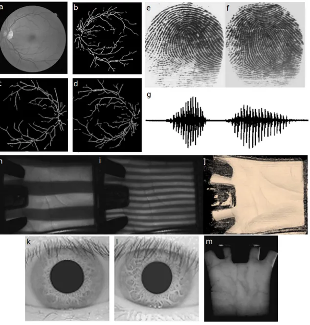
Studies of physical and behavioural traits for recognition purposes are known as biometrics. Be-ing specific of an individual, they guarantee one’s identity in security control situations. A well known example of a biometric characteristic are fingerprints, being most widely used [1]. It is theoretically impossible to find any two individuals with the same fingerprint [2]. This is a cru-cial property of a biometric characteristic: to be unique for each person. Other equally important aspects regarding biometric characteristics are universality, as they have to be present in all indi-viduals; and permanence, so they are constant during one’s life. Moreover, they should be easy to extract. At present time, there is research activity in a broad range of biometric characteristics which can be divided into physical and behavioural. Physical are, for instance, fingerprints, iris, retinal capillary structure, face, and hand recognition. Examples of behavioural traits are voice and handwriting. Figure1.1illustrates several biometric characteristics.

Biometric systems can be used for identification and verification purposes. In all cases there should be a database where biometric features from a set of individuals are stored. In an iden-tification task, the role of the system is to compare an input with all the entries in the database and verify if there is a match, thus detecting the presence of the individual in the database. In a verification task, the algorithm checks if an individual is whom he claims to be. To compare any kind of biometric characteristics it is necessary to represent them in a stable fashion. For instance, it is not feasible to directly compare images from two palmprints, as it is practically impossible to place the hand in the exact same position in different occasions, producing slightly different images that have to be compared in some way. This is the most crucial aspect and can be divided into two tasks:

1. Represent a characteristic trait in reproducible and stable features that resist input variability.

(14)

Figure 1.1: Biometric characteristics. a) Retinal fundus image and b) correspondent vascular-ization. c) and d) are examples of retinal processed images from different persons. All retinal images were taken from ref. [3]. e) and f) are fingerprints from twin sisters [4], with noticeable differences to the naked eye. g) represents the pressure-time plot of the /eda/ utterance (complete unit of speech) [5], from which spectral information can be retrieved to identify a speaker. h) and i) depict the illumination system from which 3D palmprint information j) is retrieved [6]. k) and l) are iris from two different persons [7]. m) depicts detection of palm veins using infra-red lighting [8].

(15)

Introduction

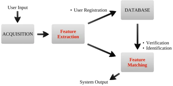
These two questions are in the core of a biometric system and are addressed by most of the research in the field. Its importance is highlighted in figure1.2where the layout of a biometric system is depicted.

Figure 1.2: Typical scheme of a biometric system.

1.2 Palmprint Biometric Recognition

1.2.1 Motivation

During the last years there has been an increasing use of automatic personal recognition systems. Palmprint based biometric approaches have been intensively developed over the last 12 years be-cause they possess several advantages over other systems.

Palmprint images can be acquired with low resolution cameras and scanners and still have enough information to achieve good recognition rates. In this case, the discriminant informations relies in palm lines and texture. However, if high resolution images are captured, ridges and wrinkles can be detected, resulting in an image similar to fingerprints. Forensic applications on latent palmprints typically require high resolution imaging, with at least 500 dpi [9].

According to the classification in [10], palmprints are one of the four biometric modalities possessing all of the following properties:

• universality, which means the characteristic should be present in all individuals; • uniqueness, as the characteristic has to be unique to each individual;

(16)

• Permanence: its resistance to aging;

• Measurability: how easy is to acquire image or signal from the individual; • Performance: how good it is at recognizing and identifying individuals; • Acceptability: the population must be willing to provide the characteristic; • Circumvention: how easily can it be forged.

The other three modalities are fingerprints, hand vein and ear canal. For instance, iris based methods, which are the most reliable, require more expensive acquisition systems than palmprint systems. Face and voice characteristics are easier to acquire than palmprints, but they are not so reliable. Overall, palmprint based systems are well balanced in terms of cost and performance.

1.2.2 Objectives and contribution

The main objective in this thesis is to build a full recognition system, from the pre-processing to the classification phase. It is divided in two main tasks. First, principal line detection, and then, recognition based in textural information of principal lines.

In the principal line detection part, two methods are developed using graph search methods. To our knowledge, graph search line detection is on of the more advanced methods employed in this field. The developed methods can be easily improved and therefore constitute a framework for future work in palm line detection.

In the recognition part, Haralick’s features are used for the first time in palmprint recognition. The texture feature extraction method, along with the concept of texton dictionary open a new branch in feature extraction for palmprint recognition purposes.

1.3 Description of Contents

Here a brief summary of the structure of this thesis is presented.

In chapter2— State of the Art — a review of palmprint feature extraction and matching in the last decade is presented. The main approaches are discussed and insight about directions for future work is given.

The pre-processing steps used in this work are explained in chapter3. These are noise filtering and extraction of a region of interest.

One of the major components is the development of line detection methods. Chapter4— Prin-cipal Lines Detection — describes two different implementations using a graph search approach.

In chapter5a method to compare palmprints based in texture of principal lines is developed. Finally, chapter6draws the main conclusions from the work developed in this thesis.

(17)

Chapter 2

State of the Art

Comparing two palmprints requires the extraction of useful information that is ideally indepen-dent of acquisition conditions, such as hand positioning, palm ageing, illumination and dirt. This process is called feature extraction. Then, to assess one’s identity, these features will be compared in a process called feature matching. Most of the research is devoted to these two phases of a biometric system.

Following this research trend, this thesis does not scope the acquisition devices and the oper-ational performance of the palmprint recognition system. It is focused on the algorithmic com-ponent of the process. In this chapter, a review of the state of the art in feature extraction and feature matching is presented. Methods used to evaluate performance of different algorithms are also discussed.

The way research is presented in this chapter is somewhat different from a recent review [11], in which a palmprint recognition method is classified into a group according to one of the image processing algorithms used. However, with such scheme it is impossible to organize all methods for palmprint recognition without overlapping the classification, because in each method many techniques are used, and new work often arises from new combinations of techniques previously used.

Here, different techniques are categorized according to the stage of the process in which they are used. First is the preprocessing stage which involves creation of a coordinate system to align palmprint images. Next, is feature extraction, the stage that contemplates more variety in the techniques and methods used. Then, is feature reduction, which is a form of selection of extracted features. Finally, some aspects of the classification stage are presented.

Different algorithms arise from different combinations in each of these stages. Examples are given for each technique, contextualizing the methods used in every stage so the reader can understand the importance of a given stage in the full process. References are often repeated because they serve as example in more than one stage.

(18)

2.1 Local vs global features

This is a core characteristic of a palmprint recognition methods. To associate extracted features with specific locations in the palm it is necessary to establish a coordinate system to enable valid comparisons between different images. While almost all methods employ local specific features, there were some implementations using global features.

2.1.1 Global features

These are methods that code information retrieved from the whole palmprint at once. Therefore, no spatial information is used, and extracted features are related to the whole palm. Research using global statistical features was short because it compromises performance by discarding spatial information. Such methods can discover what features a palm has, but not where those features are located in the palm.

Examples:

In [12] palmprint images are converted to three wavelet domains, which are sensitive to differ-ent oridiffer-entations, therefore including information about line oridiffer-entation. Then, features of wavelet sub-bands such as sparseness and energy are used to describe a palmprint. Verification is per-formed by calculating the difference between features from two palms. A weighted distance scheme was developed for this task.

Invariant Zernike Moments were used by Pang et al. [13] to describe a palmprint. They compare vectors with moments of different orders using euclidean and Norm 1 distances. Higher order moments have more information for personal recognition because they relate to finer details. Li et al. used a Modular Neural Network as a classifier for the same features, instead of simple Norm 1 or euclidean distances [14].

2.1.2 Local features and coordinate systems

Methods including feature vectors associated with spatial location exhibit superior performance. Most of the systems create a square in the middle of the palm [11]. In most cases, the coordi-nate system is used to extract the region of interest (ROI), and subsequent feature extraction is performed on the ROI. If the coordinate system is well defined, ROI’s from different images are aligned — correspond to the same area in the palmprint — and comparison between feature vec-tors is meaningful with regard to spatial information.

Relevant approaches:

A common approach is to use finger valleys as reference points. Typically the used valleys used are between index finger and mid-finger and between ring finger and last finger. There are numerous approaches to detect such points [15,16,17,18,19].

(19)

State of the Art

Figure 2.1: Coordinate system based in reference points in finger valleys. In a), finger valleys are used as reference points (white X marks), on which a coordinate system is established. The resulting region of interest is depicted in b). Adapted from ref. [15].

In figure2.1, a squared ROI is extracted based on finger valley reference points. It is defined in such a way that it is centered on the line that crosses the two points. This system is similar in several methods, as reviewed in [11].

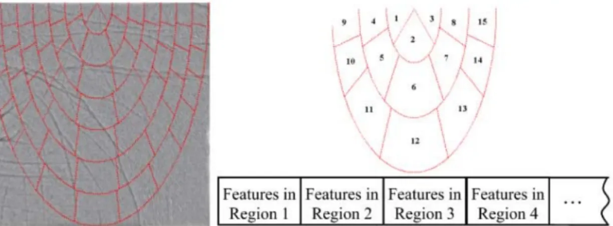
The work in [20] defines subregions on a ROI, and elements in the feature vector are associated to the subregions. Of course, the ROI position depends on reference points, which are the three finger valleys between all fingers but the thumb and index fingers. These subregions are based on ellipses (figure2.2).

A different approach is used in [21], where features are retrieved in concentric circles. In [22], authors use datum points (characteristic points) in principal lines to define a coordinate system and align images. This was implemented on off-line palmprint images, which are inked and printed on paper, and it’s out of date. However, the concept of using lines as a reference for coordinate systems was proposed for on-line palmprint images [23]. This method uses points located on palm lines as reference, which is more suited to account for skin stretching. Methods that use finger valleys as reference are more subject to skin-stretching associated errors. However, there is not enough research yet using this method to support its theory.

2.2 Feature extraction

2.2.1 Line associated features

Visually, lines are the most evident characteristic of palmprints. If one is asked whether two palm-prints belong to the same individual, the most natural comparison is made through the position and aspect of lines. Because of their importance, some of the methods developed use edge detectors for feature extraction.

Some of the best performing methods extract features strongly related to line orientation. This is probably one of the most stable features regarding variant conditions at acquisition time. Some examples of these methodologies are detailed below.

(20)

Figure 2.2: Elliptical coordinate system. In a), an elliptical coordinate system is defined inside a region of interest. Values in the feature vector depicted in b) correspond to the subregions defined in a). Adapted from ref. [20].

Examples:

In [19], sobel operators are used to detect lines. Summation of sobel response over columns and rows originates two histograms, which are used for classification by Hidden Markov Models. In [24], a filter based approach based on Radon transform is implemented to detect lines. Superposition is used to match palmprints.

In [25], line segments are detected by convolution with 3 × 3 operators that approximate the shape of a straight line. Because the detected segments are considered to be straight, it is possible to represent them by their end-points. Matching between two images is performed by comparing coordinates of the segment end-points from the two different images.

In [26], lines are detected with canny filter. The extracted ROI is divided in subregions and in each subregion properties associated with canny response and line orientation are kept. Euclidean distance is used for matching.

2.2.2 Gabor filters

In PalmCode approach [15], images are convolved with one Gabor filter. For each location in the region of interest (there are 32 × 32 locations), Gabor response is converted to a binary format. This can be considered a feature reduction method, as Gabor response will be 1 or 0. Afterwards, hamming distance is used as a classifier. This approach was classified as texture based because Gabor filters are often used as texture discriminators. Because these filters can model lines ade-quately, subsequent methods used them to detect line orientation [11].

Other examples of work using Gabor filters is found in references [27,21,20].

2.2.3 Invariant features

Some computer vision problems require features invariant to rotation, scale and stretching. As image palms are subject to these conditions, invariant features were used in palmprint recognition.

(21)

State of the Art

Examples:

Scale Invariant Feature Transform (SIFT) [28] was used in ref. [29] to extract features, al-though the results are not as good as other methods.

In [14], Zernike invariant moments are used as features. In [30], the feature vector is composed by Hu invariant moments.

In [31], a rotation invariant texture descriptor — local binary pattern (LBP) [32] — is used to extract features.

2.2.4 Wavelets

Wavelets are a mean of extracting useful information from images. There are some examples of articles using wavelets for feature extraction.

Examples:

Low- and high-pass images are originated through Haar wavelets and regarded as features. Dimensionality reduction is performed on sub images using Independent Component Analysis (ICA) [33].

In [34] M-band wavelets are used to decompose the image. L1-norm and variance of sub bands

compose the feature vector.

2.2.5 Image subspace

Approaches to determine statistically relevant subspaces, such as ICA, Principal Component Anal-ysis (PCA) or Linear Discriminant AnalAnal-ysis (LDA) can be directly applied to images. The result is a feature vector by itself. Although it is not an intuitive approach to identify personal character-istics in palmprints, the purely statistical information is useful.

Examples:

An example of image subspace as features is the work presented by Wu et al. [35]. Images are treated as a point in a multidimensional vector and LDA is used to reduce its dimensionality. In the training phase, a projection is computed using a set of pictures. This determines the Fisher’s space for the given training set. Then, in the testing phase, images are projected accordingly to the previous phase, reducing its size while keeping relevant information from pixel values. Later, in the classification stage, euclidean distance is used as matching function.

In [36], images are projected with PCA into a subspace, which the author name “eigenpalms"".

2.2.6 Other

Other features were used for palmprint recognition. Two examples are the use of fractals [37] and phase component of Fourier transform [38].

(22)

2.3 Feature selection

In virtually every type of data one can think of, there are some points more relevant than others. Methods to find statistically important components of data have been applied, such as PCA or LDA. The initial data is thus represented in a subspace where important information is more evident.

These methods have been applied to palmprint recognition in different ways. Here, examples of direct application to features extracted from images are shown.

Application of subspaces directly to images was discussed in the section2.2 — Feature ex-traction.

2.3.1 Specific property coding

Following Palmcode [15], different approaches using Gabor filters were implemented. In Com-petitive Code [39], each point in the palm is considered to belong to a line and an orientation is assigned by finding the maximum output of six Gabor filters with different orientations. The fusion code [40], a similar approach is implemented with Gabor filters with four orientations. An-other approach is reported in [41], where response of Gabor filters with three different orientations are encoded in three bits.

2.3.2 Subspace

A good example of using subspace approaches is described in [42]. Magnitude from Gabor filters is useful to take information from images. 40 different filters combining eight different directions and five scales were used. As the images are 128 x 128, the total number of features is 128 × 128 × 40= 655360. AdaBoost, an adaptative machine learning algorithm, and LDA, are used to reduce the number of features. This is done by training the algorithm towards separation of self classes and external classes. The resulting number of features is less than 200. There is no discrimination between which gabor filter are being used, or from where in the palm are features being taken, because they do it all at once.

2.3.3 Clustering

An example of clustering algorithms is a subsequent work to Competitive Code [39]. In this approach Gabor filters with six different orientations are used to extract line orientation. An im-provement to this approach using a clustering algorithm was related in [43] where filters with 180 orientations were used to extract features. Through clustering with Fuzzy C-Means algorithm the 180 orientations are clustered into six centroids. Implementing Competitive Code with Gabor filters oriented as the detected centroids results in improved performance while using the same amount of information.

(23)

State of the Art

2.4 Classifiers

Euclidean distance is most used measure for matching feature vectors, although other distances have been employed. However, the use of learning methods and more advanced classifiers often results in improved performance. Here, examples of classifiers used for palmprint recognition are given.

In [18], statistical properties calculated over the response of edge detectors are used to feed a Neural Network. In [14], Neural Networks are used to match features based on Zernike moments. In [19], lines are detected with sobel operators. Histograms of sobel response summed over X and Y axis of the image is used to train an HMM.

Use of SVM’s to match features based in wavelet decomposition was stated in [44].

These are representative examples of standard classification procedures in palmprint recogni-tion.

2.5 Performance assessment

2.5.1 Databases

To correctly assess performance of different methods it is advisable to run large scale tests. Here, four examples of palmprint databases are shown.

PolyU Palmprint Database

PolyU [45] is the most widely used low-resolution palmprint database for algorithmic research considering recognition purposes. It is comprised of 7752 images from 386 different users. Users provide either the left or the right hand, but not both. On average, there are 20 samples per user, taken in two sessions. Visually, it is possible to identify more variability between images between different sessions. This happens because there is time lapse between the sessions, which makes the results closer to what happens in operating systems. Due to the use of pegs, hand positions are restricted simplifying preprocessing stages.

CASIA Palmprint Database

The CASIA Palmprint Database [46] is similar to PolyU although smaller in size. There are no pegs to restrict hand positions. Users lay the back of the hand on a dark surface and a fixed CMOS camera is used for image acquisition.

IIT Delhi Touchless Palmprint Database

This database [47] uses a normal camera to take pictures to hands standing in the air, without any support. This increases the variability in hand positions. There are two problems to deal with in such conditions: hands can be at different distances and inclinations relative to the camera,

(24)

distorting the images. These factors increase the complexity of pre-processing steps necessary to align images before any comparison is made between different hands.

Hand Geometric Points Detection Competition Database

In order to explore influence of hand position in acquisition of geometric features, a database with-out pegs or any position constraints during acquisition was created [48]. This is a very challenging database because it requires extraction of characteristic points to align images before any further steps. However, positional freedom caused some palms to be partially hidden or severely distorted, compromising its usage in palmprint recognition.

2.5.2 Measures of performance

Genuine matches (or true positives) are matches between palmprints from the same user. Impostor matches (or false positives) are matches between different users. Performance of an algorithm is assessed by how well the system can separate genuine matches from impostor matches in a database. To measure that separation, the system outputs a distance between the palmprints, which should be higher in the case of an impostor match.

There are two tests to evaluate performance: • Verification

• Identification

In verification tests it is assessed whether the method can prove if an individual is who he claims to be. This is the same as asking the question: Is this person who he claims to be? These tests are performed by comparing every possible pair of palmprints in the database, and classifying in genuine and impostor matches. An operating threshold determines what is considered a genuine or an impostor match (if the individual is whom it claims to be). If the distance measure is correct, the system is able to correctly separate genuine from impostor matches.

In identification tests, the system aims to identify an individual in a database. The system should also be able to discriminate whether the individual is present in the database or not. Tech-nically, an input is compared with a set of palmprints in a database (to simulate a user database). The system uses the distance measure to identify the best match (shortest distance) with the entries in the set. That distance has also to be smaller than the operating threshold, to validate identifica-tion of the input palmprint and guarantee that unregistered users are not accepted. There are more errors in this test, because in addition to the errors arising from the operating threshold, genuine matches have to correspond to the shortest distance in the whole user set. A greater number of users in the set generates more errors.

Figure2.3illustrates palmprint distance measures for a set of genuine and impostor matches. Impostor matches have greater values than genuine matches, which is expected, but there is some overlap between two distributions, leading to classification errors. The operating threshold should be set in order to minimize such errors. The true positives and false positives are on the left of the

(25)

State of the Art

threshold. True positives arise from the elements in the genuine distribution, while false negatives are the elements in the impostor distribution falling under the threshold value. The same concept is valid for true and false negatives, with the genuine distribution originating false negatives (false rejections). 0 0.1 0.2 0.3 0.4 0.5 0.6 0.7 0.8 0.9 1 0 0.2 0.4 0.6 0.8 1 1.2 Matching Distance F re q u en cy o f p a lm p ri n t p a ir s _Impostor Distribution TP FN TN FP Genuine Distribution Operating Threshold

Figure 2.3: Genuine and impostor distributions as function of a similarity measure. FP, FN, TP, and TN denominate false positives, false negatives, true positives and true negatives, respectively. The red vertical line represents the operating threshold separating true and impostor matches.

Value of the operating threshold can be set lower, to increase security, or higher to decrease false rejections. A Receiver Operator Characteristic (ROC) curve is created by plotting true and false positive rates for all possible threshold values (figure2.4). It is possible to assess all relevant rates at once: GAR, FAR and FRR (Genuine Acceptance Rate, False Acceptance Rate and False Reject Rate). Genuine accepts are genuine matches correctly classified. False accepts are impostor matches classified as genuine matches. False rejects are genuine matches classified as impostor. The equal error rate (EER) can be estimated from the ROC curve, and corresponds to the point where FAR and FRR have the same value.

(26)

0 0.1 0.2 0.3 0.4 0.5 0.6 0.7 0.8 0.9 1 0 0.1 0.2 0.3 0.4 0.5 0.6 0.7 0.8 0.9 1

False Acceptance Rate

G en u in e Ac ce p ta n ce R a

te FAR True negatives

FRR false negatives

false positives

GAR true positives

EER

Equal Error Rate

Random prediction

Figure 2.4: Toy ROC curve. For all possible operating thresholds, the genuine and false accep-tance rates are calculated and plotted (black line). For a given point (red circle) FAR and GAR are represented as the distances to the Y and X axis, respectively. A random matching algorithm is represented by the continuous red line. The intercept between the dashed red line and the ROC curve represents the EER.

(27)

Chapter 3

Pre-processing Notes

3.1 Region of interest

Most of the existing works use small regions from the palmprint, wasting a significant portion of the palm. Intuitively, the more area used for feature extraction and matching, the better the recognition. Of course, this might increase computation time. We implemented a method to extract a region of interest (ROI) that maximizes the area used.

The image is converted to binary format using the Otsu’s algorithm [49], which is composed of white (ON) and black (OFF) pixels. Then, three morphological operations are performed:

• Closing, with a circular structuring element of 8 pixels in diameter. This eliminates holes in the image.

• Opening, with a circular structuring element of 5 pixels in diameter. Small objects origi-nated from noise are deleted with this procedure.

• Erosion, with a circular structuring element of 8 pixels in diameter, ensuring the region of interest is completely inside the palm.

The option for the size of morphological operations is adequate since the resolution of the image is 180 × 240, approximately.

At this point the left bottom and top borders of ROI are defined. Now, it’s necessary to set the left border of the ROI. This is done by calculating the number of ON pixels in each column. This value will be zero on the left of the image, where no portion of the palm is present. Towards the right side, the number of ON pixels starts increasing because the fingers are present in those columns. The maximum value is present after the fingers zone, and this is where the left border of the ROI should be set. The column chosen for left border is 8 pixels to the right from the first column in the image (counting from the left) to have 86% of the maximum of ON pixels (figure

3.1). The value of 86% was determined empirically.

(28)

0 50 100 150 200 250 300 350 400 0 50 100 150 200 250

Column index

Nu

m

b

er

o

f

o

n

p

ix

el

s

Number of on pixels 86% maximum on pixels

Figure 3.1: Finding left border of ROI. In the binary image obtained after morphological oper-ations, the number of ON pixels in each column is represented (black line). The red line is set at 86% of the maximum of ON pixels for a given image. The left border of ROI is placed 8 pixels to the right from the first column (counting from the left) hitting the red line.

Figure 3.2: Extraction of ROI. Original image is in a). Through morphological operations, the mask in b) is computed. The region used further in this thesis is represented in c).

(29)

Pre-processing Notes

3.2 Extracting mid-frequency information

There are two types of noise that can affect performance of methods developed: high frequency noise and low frequency noise. High frequency noise arises from the resolution limit of the camera and corresponds to strong local variations in pixel values. A pixel with high intensity inside a palm line is an example of high frequency noise. Low frequency noise is originated from the three-dimensional shape of the hand, which makes some areas of the palm to be illuminated differently. To reduce both types of noise in input image I, two Gaussian filters are used for convolution, adequate to respond to different frequencies. This methodology is called Difference of Gaussians (DoG) and is commonly used as an edge detector, but in this case its use is as a band-pass filter. The filtered image IF is calculated as follows:

IF= (I ∗ G3×3_σ=0.5) − (I ∗ G20×20_σ₌₂₀), (3.1)

where G3×3_σ_=0.5 is a 3 × 3 Gaussian operator with σ = 0.5 which eliminates high frequency noise. Convolution with a Gaussian operator of size 20 × 20 and σ = 20 detects low frequency information which is subtracted.

Finally, image is mapped to the range[0, 255]:

IF= 255 ·

IF− min(IF)

max(IF) − min(IF)

(30)

(31)

Chapter 4

Principal Lines Detection

Edge detection - is a universal task in computer vision and algorithms for this purpose exist since long time ago. There are a multitude of different algorithms suitable for a different range of problems. At the time being, a search for “Edge Detection” on IEEE Xplore engine retrieves over 18.000 results. However, only very few were applied to palmprint images. Some are standard edge detection techniques, such as the Canny filter [50] used in ref. [51], or the Sobel operator used in ref. [52]. In other works new methods for palm line detection are developed [53]. Line detection usually uses detected edges to reconstruct lines, as for instance, the Hough transform [54] used in ref. [55]. In this thesis, two methods based in graph-search for edge following are implemented and tested.

Principal lines are among the most stable features in palmprints, considering natural ageing processes and changes in acquisition conditions. Therefore, it is of great interest to detect them accurately. Actually, there were previous attempts to detect principal lines [56], as they can be used in several ways to improve palmprint recognition. It is possible to directly compare the shape of palm lines by superposition methods [57]. Some features can be extracted directly from palm lines [52] and be used to compare different hands.

One of the mandatory processes in a significant number of recognition systems is the establish-ment of a coordinate system, which is based in defined geometric points. Usually, these points are the valleys of the fingers [11]. However, this procedure might be inappropriate since the reference points are external to the palm and skin stretching allows a wide range of palm positioning. Using reference points inside the palmprint — based in principal palm lines — would be more efficient, as it would diminish the errors associated with skin stretching[23].

One of the main objectives in this thesis is to develop a method that avoids coordinate systems, which are subject to alignment errors. The proposed approach (Chapter5) takes textural informa-tion from regions around the detected principal palm lines, discarding spatial informainforma-tion as the extracted texture has no association with a specific position in the palmprint. Also, orientation

(32)

of the lines is not included in any fashion in the feature vector. This procedure will give strong insight on the importance of line texture as a feature for palmprint recognition.

4.1 Related work in palmprints

In this section, two existing methods for palm line detection are detailed: gaussian derivatives as used in [58]. Gaussian derivatives are a standard edge detection algorithm, used in several edge detection problems. Modified finite radon transform (MFRAT) was specifically created for palm line detection. These two were chosen for being representative examples of edge detection algorithms.

Gaussian Derivatives

Calculating derivatives of an image is a standard procedure to detect edges —lines in this case. Here is a summary of the methodologies found in ref. [58]. First, image is smoothed by 1-D Gaussian filtering with variance σs, which has influence on the smoothness of the lines that can be

extracted. The smoothed image Isis calculated as follows:

Is= I ∗ Gσs (4.1)

where “∗” denotes the convolution operation, “I” is the original image and “Gσs” is a one-dimensional

Gaussian function. Then, first and second order derivatives are calculated by a sliding window that performs convolution with derivatives of a one-dimensional Gaussian function. With this procedure line detection is direction specific, thus it is necessary to repeat the method in several directions, which are 0° 45° 90° and 135°. These are derivatives of 1-D Gaussian functions with variance σd, which has selectivity on width of detected lines. The mathematical formulation is as

follows:

I_θ0 = Is∗ (θG0_σ_d)T (4.2)

I_θ00= Is∗ (θG00σd)

T _(4.3)

where “T” is the transpose operation, “∗” is the convolution operation and “θ_G0

σd” and “ θ_G00

σd”

are the first and second-order derivatives in direction “θ ” of a one-dimensional Gaussian function with variance “σd”.

Edges are detected by looking for the zero-cross points of the first derivative, which indicates the presence of an edge. At that point, the second derivative is used as a measure of intensity of the detected edge. A line in a palmprint digital image is represented by low intensity pixels surrounded by high intensity pixels, which can be detected like edges. The first-order derivative is negative as the filter passes from the surroundings into the line, and is positive as the filter goes out of the line into the surroundings again. This obligates existence of a zero cross point. For a stronger line, the first-order derivative will produce more negative values before the line and more

(33)

Principal Lines Detection

positive values after the line. This implies that a strong line has a high second-order derivative. This is why it is used as a measure of line intensity. Check figure4.1for a graphical explanation.

0 5 10 15 20 25 30 35 40 −1 −0.8 −0.6 −0.4 −0.2 0 0.2 0.4 0.6 0.8 1 Pixels No rm a li ze d V a lu es Image intensity 1st_derivative 2nd_derivative

Figure 4.1: Detecting lines with first and second order derivatives. The dark black line repre-sents a slice of a palmprint image. The slice transversally crosses a palm line at pixels 13 to 19. As palm lines are represented by darker pixels, the slice’s intensity profile has a valley when it crosses the line. In the center of the line, first order derivative is zero while second order derivative has its maximum value.

As derivatives are sensible to noise and false edges are detected, there is the need to find a threshold to correctly separate lines from background. However such procedure results in broken lines because some of its segments fall under the threshold. In ref. [58] hysteresis thresholding was used to overcome this issue. It consists in applying two thresholds on the value of the second derivative, Thighand Tlow. Lines above Thighare considered strong lines and are always kept. Lines

above Tloware kept only if they contact strong lines. Tlowis the minimum of the non-zero values,

which means it is considering all detected lines. Thighresults from applying Otsu’s method to the

non-zero values.

Modified Finite Radon Transform

In this work authors extract lines using a modified finite Radon transform (MFRAT). The Radon transform consists in projecting a bi-dimensional function, such as an image, into several 1-D projections [59]. The set of 1-D projections is performed in the range of 0° to 180°. A projection is the summation of image intensity along all parallel axis to an imaginary line with the angle specified. Despite the mathematical description above, the proposed MFRAT looks more like a filter than a transform. In fact, it is not possible to restore the original image from the output. It consists in sliding windows that convolves with the image. If the center pixel of a window falls in a line, and the rest of the mask is aligned with that line (low pixel values), the filter output will be

(34)

minimum, indicating presence of a line. Thus it is necessary to have enough filters to represent all possible line directions. There are 12 sliding images, each for a different angle. Six of them are represented in figure4.2.

Figure 4.2: Windows used in ref. [60]. Only windows from 15° to 90° are shown.

As this sliding window screens the image pixel by pixel, two new images are generated. One is the energy image, which has the value of the minimum summation for every angle window. The other is the angle image for which the angle corresponding to the lowest energy value is kept. It is important to mention that the average of each window is subtracted before the filtering operation occurs, causing the method to be sensible to line direction and shape rather than differences in pixel values.

The angle image is used to split energy image into two sub-images. Energies associated with line angles between 0° and 90° are stored in one sub-image and energies associated with line angles between 90º and 180º are stored in another sub-image. It is considered that principal lines are in one of the two sub-images. Radon transform is used to find the sub-image with more line intensity, and that will be considered the principal lines sub-image. This has an inherent drawback, since principal lines can be present in both images, as the angle chosen for division is independent of the images.

4.2 Shortest paths as edge detector

4.2.1 Context and concept

To understand what a shortest path is it is necessary to introduce some graph concepts. A graph is a representation of a set of nodes, which are connected by a set of arcs. In the case of image processing, we consider the pixels of an image the nodes of a graph, where arcs conceptually connect pixels to each other. Usually, each pixel is connected to its eight neighbours.

According to graph theory, if arcs connecting nodes have a weight associated, the graph is called an weighted graph. The shortest path between two nodes is the path formed by the arcs summing the least weight possible. If one properly uses image properties to weight arcs, shortest paths will exist over the edges.

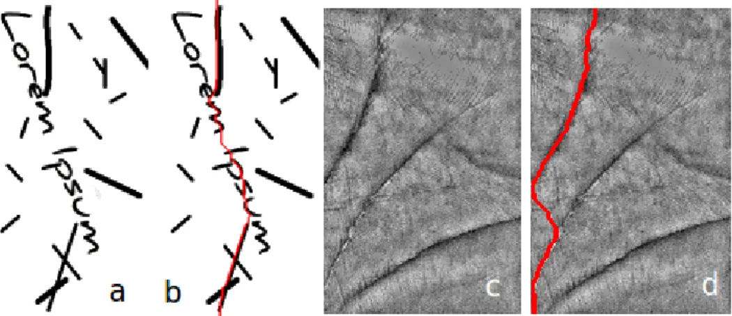
This concept was introduced because of its ability to detect connected edges even in the pres-ence of noise[61]. Other methods would produce fragmented lines, which are more difficult to interpret computationally.

(35)

There are other approaches to avoid segmented lines detection, like active contours (also known as snakes). With this approach, a line is initialized. Then, external and internal forces operate to guide the line towards the edge. Internal forces regard line shape and length, to approx-imate detection to the shape and size of the expected output. External forces attract the line to the edge. This approach is useful in the detection of objects, because the initial line can be closed around a probable location of the object[62].

4.2.2 Description of the algorithm

In the image derived graph, the distance between two pixels is dependent on characteristics of those pixels. Because palm lines are regions of the image with low intensity level, the weight of an arc is set to be lower if pixel values are lower. This results in shortest paths to exist on darker regions such as palm lines, thus making shortest path algorithm work as a line detector. This concept was already used for staff line detection in musical scores [63], yielding promising results.

The concept described for line detection works best if the shortest path is computed between two nodes on the edges of a line. However, it is harder to detect the ends of a line than the line itself, making it necessary to screen for the shortest path over a reasonable area.

Because of this, the implemented algorithm searches for the minimal path between a set of nodes A and a set of nodes B. Practically, A and B are the first and last rows of pixels in a rectangular image.

The graph search problem in line finding is much simpler (lines have to keep the same di-rection, can’t go back and forth), the implementation of known algorithms [64,65] is simplified. Costs of several paths are computed row by row, from A towards B. There are three conceptual elements involved:

• Weight matrix W(i, j), which is a matrix of the same size as the image that assigns a weight for each pixel, based in, for example, grey level intensity. In this method the weight matrix are the pixel values themselves;

• Cost matrix C(i, j) that stores cost values of several paths;

• direction matrix D(i, j) that has information about the change of direction of each path in every pixel.

The weight of a path between two pixels is calculated from the weight matrix. It is defined as the geometric mean between the vales of the two pixels, multiplied by the euclidean distance separating the two pixels. The geometric mean gives a lower value to the path linking a dark to a bright pixel than to the path linking two intermediate pixels.

For a pixel P(i, j), where i iterates over rows from top to bottom, and j is the index of the pixel in that row, three paths are considered: the path arising from the pixel immediately above: P(i − 1, j), the path arising from the top-left pixel P(i − 1, j − 1) and from the top-right pixel P(i − 1, j + 1). The cost for each of these three paths is the weight of the considered path linking

(36)

the previous pixel to the current one, plus the cost of the already calculated path in the pixel where the path is coming from: Cost = W (i, j) + C(i − 1, j + d), where d = {−1, 0, 1} for the top-left, top-center and top-right pixels, respectively. The minimum of these three possible values for Cost is stored in C(i, j) and the corresponding direction value d in D(i, j).

In this way, the value of each element in C(i, j) is the cost of the shortest path linking the correspondent pixel to the first row in the image.

As the algorithm runs over the rows, cost values increase as they correspond to the sum of all weights associated to pixels forming growing paths. For a pixel j in a row i, there is only one path, the cost of that path is C(i, j) and the indexes of pixels forming that path can be retrieved from the direction matrix D. In the last row, the path starting from the pixel with the smallest value in the cost matrix C is the shortest path in that image. There are no horizontal connections between pixels, only vertical and diagonal, limiting paths to be inclined at a maximum of 45°. Also, paths are either top to bottom or bottom to top (is the same as the paths are symmetric) but they can’t support both directions. This means that paths will be straight forward linking top and bottom edges, without turns. It is guaranteed that the global minimum is found. Figure4.3illustrates the output of the described algorithm.

Figure 4.3: Short paths in images. Images are treated as a graph and the shortest path (red lines) between top and bottom of each image is computed. Arcs connecting dark pixels have a lower weight, forcing the shortest path to exist over long vertical and dark portions of the image. a) original toy image and b) corresponding shortest path. c) original palmprint image and d) corresponding shortest path.

4.3 Method I — Shortest paths in subregions

Using shortest path to detect line has the advantage of detecting a long, straight lines, which are characteristics of principal lines in palmprints (figure 4.3). However, it is not trivial to define where to compute the path. To solve this problem it was proposed to compute several shortest paths in subregions of the image. In this method, the image is divided in squares of arbitrary size and two shortest paths are computed in each subregion: the vertical path, linking top and bottom

(37)

edges, and the horizontal path, linking left and right edges. Figure4.4depicts the output from this implementation including square subregions of two different sizes.

Figure 4.4: Computing shortest paths in subregions of an image. a) is the original input image and d) has principal lines marked by hand. b) and c) are divided in squares 30 and 80 pixels wide, respectively. Horizontal and vertical shortest paths (yellow) are computed in each of the squares. A threshold was applied to keep the 15% (in e) and 30% (in f) darkest pixels as principal lines. Red circles mark line segments that cannot be detected as they are inclined by nearly 45°. Green circles indicate a line segment that was not detected using 80 pixel wide squares because the vertical path in that square is detecting a stronger line. Note that this problem did not occur with the 30 pixels wide squares.

As a shortest path will always be computed even if there is no line inside a square, numerous portions of paths that do not correspond to any line will exist — see figure4.4b) and c). Thus it is necessary to eliminate such path segments. Since lines are the darker pixels of the image, this property can be used to differentiate the valid pixels in the shortest paths. A threshold is applied to keep only a percentage of the darker pixels in computed shortest paths of an image. Ideally, this procedure can eliminate all extra segments while keeping pixels over the palm lines.

The two parameters in this method are:

• Subregion size (width of the square subregions in pixels) • Percentage of darkest shortest path pixels to keep (a threshold)

(38)

There are various drawbacks inherent to this implementation, and some consequences can be predicted.

First, if subregions are too big and two lines with similar orientation are placed inside the same square, it is not possible to detect both lines. Using smaller squares can solve this issue. However, smaller subregions mean more shortest paths will be computed resulting in an increased number of extra segments that correspond to no line. It might be complicated to separate the extra segments from the meaningful detections.

Second, if lines are oriented at 45°and cross subregions through adjacent borders, neither the vertical nor the horizontal path are able to track them adequately.

To issue the mentioned cases without diminishing subregion size, which could produce addi-tional detection noise, a solution is proposed. It consists in the combination of two modifications: horizontal and vertical shift of the square subregion by half its size and the rotation of the subre-gion by 45°. This results in four different divisions of the original image:

• Original subregions • Shifted subregions • Rotated subregions

• Shifted and rotated subregions

The shortest paths computed in both horizontal and vertical directions for the four subregion set-ups mentioned above are put together. In figure4.5, it is illustrated how this procedure with-draws the mentioned issues. As referred earlier, a threshold is applied to eliminate extra segments that correspond to no line.

Because palmprint images have some noise, threshold application cannot eliminate all pixels that have no line correspondence. Likewise, some pixels over lines are wrongly eliminated. This results in broken lines and lost pixels in the images. To issue this problem, the detected lines are subject to morphological dilation, which reconnects lines, followed by morphological thinning till all segments are one pixel wide. Finally, segments shorter than 5 pixels are removed.

4.4 Method II — Dynamic tracking shortest paths

Determining shortest paths is an adequate way to find where a line is but not at verifying existence of a line. This happens because a shortest path will always be detected, whereas there is a line or not. Shortest paths should be used as a procedure to detect continuous line segments. However, in the first implemented method (shortest paths in subregions), a threshold is applied to eliminate extra segments, which brakes up the lines. Then, lines are put together again by morphological operations.

One of the main advantages in using graph search methods is the detection of fully connected segments.The previous method required the use of a threshold, which broke line segments, and

(39)

Figure 4.5: Computing shortest paths in subregions of an image. a) is the original input image. b) illustrates computation of vertical and horizontal shortest paths in 50 pixel wide squares. To diminish the number of line segments that are not detected, the squares are c) rotated by 45°, e) shifted by half its size and f) rotated by 45°and shifted by half its size. Red circles point a segment that was detected after shifting the squares and green circles point a segment that could only be detected in rotated squares.

(40)

a subsequent reconstruction by morphological operations. This is a redundant procedure. To overcome this situation, a new method which requires no thresholding was implemented.

This method is based in the idea of tracking lines with small subregions. Given an already detected portion of a line, its continuation can be detected by placing a new subregion with an adequate orientation at the end of the detected segment.

Initial (seed) segments are detected from zones in the palmprint where lines almost always exist. By studying the palmprint database it was possible to identify such areas. In figure 4.6, these areas are in black. After a line segment was detected in these initial search boxes, a new subregion is placed on top of the segment, with according orientation. The new shortest path is forced to start in the same pixel in which the previous path ended.

A problem is how to detect initial segments accurately. One property of principal lines is that they exist in fixed positions in the hand. In most cases, each of the three lines starts at one of the palm borders. Three initial boxes were created to detect the seed segment for each of lines. Now from these seeds, subregions are created and another segment is detected. It is forced that the shortest path in this subregions starts at the same pixel where the previous segment ended. This process is continued till it reaches a border of the palm, meaning the line is detected even after it ended.

Initial segments for the two lines closer to the fingers have the same shape and size. The principal line around the thumb has a different set-up.

• Thumb: It starts at 1/4 from the top and ends at 3/4 from the bottom. Therefore, the height of the box is half of the image’s. From the right, it starts 1/60 and its width is 1/6 multiplied by the images width.

• Two upper palm lines (symmetric): Horizontally, the box starts at 1/8 the width of the input image and ends at 5/8, which is slightly after the middle. The height of the box is 1/6 of the image’s height. It starts at 1/60 from the top and bottom of the images, in order to detect two different lines.

The orientation update after each shortest path detection for the tracking squares is computed taking the first and last pixels of that path, so the next square is aligned and its rows are perpendic-ular to the axis crossing the first and last pixels. The initial pixel for the next box is the last pixel in the path.

Figure4.6illustrates the algorithm described.

4.5 Performance evaluation

4.5.1 Ground truth dataset

In order to compare different methods, principal palm lines of some images were hand-marked. In total, 83 images from different users comprise the ground truth dataset. It was tried to have a balanced number of easy and difficult images. In some of the more difficult images it is hard to

(41)

Figure 4.6: Illustration of method II. a) shows detection of the line around the thumb. b) and c) are the detection of the other lines. Initial search boxes are in black, tracking boxes in white, and detected path in green.

define the lines, and the criteria used is subjective. However, this dataset will prove efficient in evaluating algorithm performance because it comprises a reasonable number of samples.

It was considered that all palm prints have three principal lines. This is a contradiction to the findings in ref. [66] which claims that palm prints can have 1, 2 or 3 principal lines. However, it is possible to visually identify three lines in all of them, although some are much weaker and probably not detected by the methods used in those works.

Figure4.7shows some examples of the ground truth dataset.

Figure 4.7: Images in the ground truth dataset. Hand-marked principal lines used as ground truth to evaluate performance of different methods.

4.5.2 Distance measures

In each image, the distance of detected lines to the ground truth is taken as a performance indicator. Of course, the smaller the distance, the better is the method. Each pixel is considered as a point in a bi-dimensional Cartesian space and euclidean distance between the two sets of points is measured.

(42)

Consider two sets of points A and B corresponding to the lines in two images. The distance of any point p in A to the whole set B is the distance of p to the closest point in B. This is also called the infimum of the distances between p and all points in B.

The average distance from A to B — Davg(A, B) — is defined as the average of the distances

from all points p in A to B.

The Hausdorff distance of A to B — Dhaus(A, B) — is the distance of the furthest point p in A

from B.

An interesting aspect of distances between sets of points is that it is not a symmetric measure. This means that D(A, B) is not that same that D(B, A). It is possible to take advantage of this property to retrieve useful information about algorithm performance.

The distance of an image to the ground truth D(Detection, GroundTruth) is low if all pix-els in detected lines correspond to a pixel in the ground truth. But consider the case in which only one pixel was detected and it was near a line in the ground truth. The distance will be low, although this situation cannot be considered a proper detection. This measurement will only be high if the detected lines are wrong, but not if there are undetected lines. This is why D(Detection, GroundTruth) is a measure of wrongly detected lines.

Distance of the ground truth to an image D(GroundTruth, Detection) is low if all lines in the ground truth were detected. But if there are extra detections, which correspond to no line, this distance is still low. This is why D(GroundTruth, Detection) is a measure of undetected lines.

Optimally, both distances are small. Figure4.8and table4.1illustrates the usefulness of these measures.

Figure 4.8: Toy images to illustrate distance measures. Three images are compared with the ground truth. Image 1 corresponds to a nearly perfect detection. Image 2 has a nearly perfect detected segment plus a false detection — false positive case. Image 3 has a correctly detected segment but misses most of the line — false negative case. The average distance of the ground truth to an image is an indicator of undetected segments, so D(groundtruth, image3) will be high. On the other hand, distance of an image to the ground truth is an indicator of bad detected lines, so D(image2, groundtruth) will be high. Results for this toy example can be found in table4.1.

4.5.3 Experimental results for Method I

In this method there are two principal parameters that affect the output. These are the size of the square subregions used and the threshold applied. This section shows results for various combina-tions of these parameters.

(43)

Table 4.1: Results for toy images in figure4.8

Indicates false negatives Indicates false positives Davg(GT, Img) Dhaus(GT, Img) Davg(Img, GT ) Dhaus(Img, GT )

Image 1 6 20 6 15

Image 2 6 20 74 187

Image 3 34 115 3 10

Performance with different parameters was evaluated as described in section4.5. The param-eters tested were all 90 combinations using:

• Size of square subregion (in pixels): 20, 30, 40, 50, 60, 80, 100, 125 and 150.

• Amount of (darkest) pixels kept: 2%, 4%, 6%, 8%, 10%, 15%, 20%, 26%, 35% and 50% The amount of false positives (wrong detections) and false negatives (undetected lines) is depicted in figure4.9, where both the distance from detection to ground truth and from ground truth to detection are shown. The distance shown is averaged within the 83 samples in the ground truth and corresponding detections. In figure 4.10 the maximum between the two distances is shown, thus including information of both false positives and false negatives. The parameters for which the maximum of the two distances is minimum are the best for line detection. In table4.2, distance measures for 4 of the best parameter combinations are shown, including both average and Hausdorff distances.

Table 4.2: Summary of best results using four different parameter set-ups Indicates false negatives Indicates false positives Square size Threshold Davg(GT, Img) Dhaus(GT, Img) Davg(Img, GT ) Dhaus(Img, GT )

40 8% 6.7 39.8 6.7 48.6

50 10% 6.6 38.5 6.7 48.9

80 20% 5.7 35.0 6.8 50.6

100 26% 6.7 38.4 6.2 46.5

4.5.4 Experimental results for Method II

There are some conditions to which performance of this method is subject, such as size of the boxes used to track lines. This is basically the same as changing size of square subregions in Method I. In order to compare performance of this method, all three implemented versions were tested with tracking squares of different sizes.

The three versions described in section4.4are:

• Version 1 : Start-point for line continuation at the end of the path in each tracking square. • Version 2 : Start-point for line continuation at 80% of the path in each tracking square.

(44)

0 10 20 30 40 50 0 50 100 150 0 10 20 30 40 50 Thr esho ldat % D(GroundT ruth, DetectedLines)

Size o_{f squa} res D is ta n ce in p ix el s 0 10 20 30 40 50 0 50 100 150 0 5 10 15 20 Thres hold at%

D(DetectedLines, GroundT ruth)

Siz_e of squ are_s D is ta n ce in p ix el s

Figure 4.9: Average distance from ground truth using different square sizes and thresholds. Detection of lines is sensitive to the size of squares (in pixels) and to the threshold applied. The smaller the squares, the more segments will be detected, therefore a smaller fraction of segments should be kept. A threshold of 10% means that only the 10% darkest pixels will be kept as detected lines. On the left, the distance between detections and ground truth is an indicator of how much segments are wrongly detected. With smaller squares and a more permissive threshold there are a lot of wrong detections — false positives. On the right, the distance between the ground truth and the detected lines is sensible to the amount of lines that are not detected. Using big squares with a tight threshold cannot detect most of the lines, explaining why such combination of parameters results in a big number of undetected segments.

0 10 20 30 40 50 50 100 150 10 20 30 40 50 Thre shol dat % Siz_{e o} f sq uar_es D is tan ce in p ix el s

Figure 4.10: Maximum of the two average distances represented in figure4.9. A good perfor-mance is achieved if both distance from ground truth to detection and from detection to ground truth are low. In this figure, the maximum of both measures is plotted in function of square size and threshold applied. Bigger squares require more permissive thresholds, such as keeping 50% of the darker segments. Interestingly, good results are achieved independently of square size, as long as an adequate threshold is applied.

(45)

• Version 3 : Same as previous but normalizing mean and standard deviation of input image. The initial search box was kept constant in all experiments. The set-up for orientation was the same as described.

Figure4.12and4.13show the average and Hausdorff distances, respectively.

Sometimes, when the track of the line is lost, the method is unable to find the line again. In this situations, there will be a bad detection (figure4.11).

Figure 4.11: Bad detections with tracking algorithm. a) shows detection of the line around the thumb. b) and c) are the detection of the other lines. Initial search boxes are in black, tracking boxes in white, and detected path in green. Tracker squares deviate from line and continue tracking in wrong directions.

4.6 Discussion

Regarding method I

The most interesting conclusion from method I is that the size of the squares works well within a large range[30, 125] (size in pixels). Of course, it is required for the threshold applied to be in conformity. This happens because the smaller the squares, the more extra segments will be produced.

Unfortunately, due to image noise, some lines appear broken and lost dark pixels not associated to lines result in false detections. Because shortest paths have the point of detecting connected segments, it does not make sense to apply a threshold on it. This causes difficulties in identifying three principal lines.

To overcome these difficulties, method II was developed.

Regarding method II

In method 2, three lines are generated in all cases. This makes it easier to regularly detect principal lines.

(46)

10 20 30 40 50 60 70 80 90 100 4 6 8 10 12 14 16

Size of tracking squares

D is ta n ce in p ix el s Average distances

Figure 4.12: Average distances for tracking algorithm. Solid lines represent D(GT, Img) and dashed lines represent D(Img, GT ), or analogously, false negatives and false positives. This method produces less false negatives but more false positives. A tracker window near 20 is optimal because it is the best compromise between false negatives and false positives. Versions 1,2 and 3 are in blue, red and black, respectively.

10 20 30 40 50 60 70 80 90 100 20 30 40 50 60 70 80

Size of tracking squares

D is ta n ce in p ix el s Haussdorf distances

Figure 4.13: Hausdorff distances for tracking algorithm. Solid lines represent D(GT, Img) and dashed lines represent D(Img, GT ), or analogously, false negatives and false positives. As seen with average distances, this method produces less false negatives but more false positives. Again, a tracker window near 20 is optimal because it is the best compromise between false negatives and false positives. Versions 1,2 and 3 are in blue, red and black, respectively.

(47)

However, the obtained results indicate that the performance of this algorithm is close to that of method I — table4.3. This might be due to the fact that if the line track is deviated from the correct position, the tracking system will not find the line again. This is particularly problematic when the lines of interest are close to each other and detected lines jump from one to the other (figure4.11). Some spatial rules can be implemented to improve the method [66].

However, less false negatives are produced. Probably, this is because lines are always con-nected, resulting in less undetected pixels.

It is visible an increase in false positives with bigger square sizes figures4.12and4.13. Maybe because a bigger search window is ineffective in tracking lines accurately, forcing the shortest path to go through wrong directions.

Table 4.3: Comparing method I and II.

Parameters Distance for false negatives Distance for false positives

Method

I _{Square size} _Threshold _D

avg(GT, Img) Dhaus(GT, Img) Davg(Img, GT ) Dhaus(Img, GT )

60 15% 5.3 33.8 7.5 52.9

80 20% 5.7 35.0 6.8 50.6

Method

II _{Square size} _D_avg_{(GT, Img)} _D_haus_{(GT, Img)} _D_avg_{(Img, GT )} _D_haus_{(Img, GT )}

15 5.0 29.8 9.1 53.3

(48)