Design of Coordinated HeNB Deployments
Rui R. Paulo
∗ ∗†Instituto de TelecomunicaçõesUniversidade da Beira Interior Covilhã, Portugal
rrp@lx.it.pt
Fernando J. Velez
† †∗Dep. de Eng. ElectromecânicaUniversidade da Beira Interior Covilhã, Portugal
fjv@ubi.pt
Giuseppe Piro
Dep. of Electrical and Information Engineering Politecnico di Bari
Bari, Italy giuseppe.piro@poliba.it
Abstract—Uncoordinated deployment of HeNBs has been widely considered, in the research community. However, due to economic or physical constraints, a coordinated deployment of HeNBs can also be considered. This work studies a selected examples of HeNB deployment. We consider the deployment of four Enterprise HeNB which serve up to 8 simultaneous users, in a building, with a geometry of 5x5 apartments. From the theoretical study on the average SINR, we have learned that the smaller the apartment areas are the higher the values for the average SINR are. The performance evolution of the system focuses on the values obtained for the average goodput, Packet Loss Ratio (PLR) and delay for the Proportional Fair, Frame Level Scheduler (FLS) and Exponential Rule (EXPRule) schedulers, with users using a video and a best effort flows at the same time. For the video flows the maximum average goodput was obtained with the FLS scheduler, but when the PLR is taken into account the EXPRule present a slight advantage. In the case of the BE flows, the EXPRule present the best performance. But the main lesson learned is that it is possible to operate a coordinated HeNB deployments without setting the transmitter power of the HeNBs to the maximum value, which can be a step to achieve a greener system.
Index Terms—Enterprise HeNB, LTE-Sim, Scheduler, SINR, Performance Evolution
I. INTRODUCTION
Traditionally a new node in a cellular network, usually an eNB, is appropriately characterized, and usually tested before is it available on the market. Nowadays, the trend for 4G systems is to have smaller and more irregular cell sizes, as 4G small cells can be deployed in any place by anyone. This possibility of deploying small cells with irregular sizes originates totally random coverage shapes [1]. This small cell nodes, technically known as HeNBs, are defined in [1] as small, inexpensive, low-power base stations that are generally consumer deployed. Although the meaning of HeNB is Home eNodeB, this nodes could be deployed in places like offices, shopping centres, industrial environments (in these cases HeNBs can be known by Enterprise HeNBs) or places where the coverage of eNBs layer are weak or even non-existent [2], [3]. In this work a maximum capacity of 8 users per HeNB is considered, as suggested in [2]. The HeNBs are not deployed in a random way or even in a totally co-ordinate way. The HeNBs have been deployed
This work was supported by National Funding from the FCT - Fundação para a Ciência e a Tecnologia, through the UID/EEA/50008/2013, CON-QUEST (CMU/ECE/0030/2017) and NEUF.
as far as possible of the external walls but sufficiently far from each other and in middle of its own apartment. This type of implementation may be due to economic or physical constraints. According to [4], Internet video streaming and downloads are beginning to take a larger share of bandwidth, and will grow to more than 81% of all consumer Internet traffic by 2021. This work studies the adoption of only four HeNBs to cover the whole building area while serving 8 users each one. The impact of video and best effort (BE) applications on the heterogeneous mobile network, it is worthwhile to study the behaviour of LTE operating the adoption of different schedulers. The main objectives are to verify the analytical behaviour of the system and evaluate the performance of three different packet schedulers. Differently from the works presented in the literature [5], [6], where a new scheduling algorithm was developed and a new bandwidth aggregation scheme was implemented in order to minimize the energy consumption, this work aims at verifying if it is possible to consider the reduction of the transmitter power of the HeNBs without compromising the overall system performance, with the existing tools.
The comparison of the results is performed for different areas and different values of the transmitter power of HeNBs. The goal is to obtain values for the average goodput, packet loss ratio (PLR) and delay as a measure of the network performance. This work also intends to optimise the range of values for the transmitter power while adopting different configurations in the studied scenario.
The remainder of the paper is organised as follows. In Sec. II a theoretical study of the average SINR is made. Sec. III presents the performance evaluation of small cells, as well as the network scenario and physical setting. Also results for different schedulers are presented. Finally, conclusions are drawn in Sec. IV.
II. AVERAGESINRSTUDY
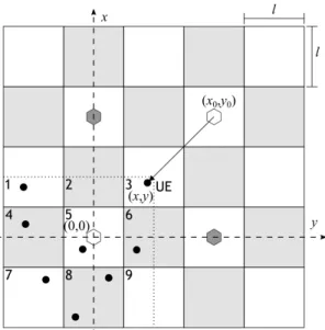
In this work we consider a single floor building with 25 apartments. The apartments are placed next to each other in a topology of a 5x5 apartments grid model. The considered topology is shown in Fig. 1. HeNBs operate with 10 MHz bandwidth and frequency reuse two, [7], [8], i.e., 20 MHz of total available bandwidth is divided into two equal parts of 10 MHz, HeNBs are represented with an hexagonal shape, two with 10 MHz bandwidth, presented with white fill, and
Fig. 1. Scenario with 4 HeNBs in the 3GPP Building topology with 25 apartments, and SINR topology.
the other two using the remaining 10 MHz, represented with lightgrey fill. The four HeNB are placed as shown in Fig. 1.
Each HeNB covers an area represented by the dotted line, meaning that each HeNB serves 1/4 of the total area of the floor, as shown in Fig. 1. Users are located inside one of such four areas served by the HeNB. When the user is served by a HeNB using a given frequency bandwidth, it will suffer interference from the co-channel HeNB. Since reuse pattern two is considered, there will be only one interfering HeNB for each user.
In general, the average Signal to Interference plus Noise Ratio (SINR) at a User Equipment (UE), placed in a position (x,y), as shown in Fig. 1, served by a cell with transmitter power PT x, can be expressed as follows:
SINR(PT x, x, y) =
¯
Pow(PT x, x, y)
(1 − α) · ¯Pow(PT x, x, y) + ¯Pnh(PT x, x, y) + Pnoise
(1)
where ¯Pow is the average received power from the own cell, α is the orthogonality factor of the codes [9]. For the sake of simplicity and according to [10] α is considered to be equal to one, and ¯Pnh is the average interference power from the neighbour cells. Pnoise is the thermal noise power and is defined as:Pnoise= −174 + 10 ∗ log10BW − 30 + N F (2)
where N F is typically 7-9 dB for LTE, and BW =10 MHz. The average interference generated by a neighbour cell can be calculated by integrating each fraction of the interfering power over the area of the affected cell. Fig. 1 shows one cell affected by interference in the origin of the coordinates and one interfering cell, at (x0, y0). By integrating over the cell area, the average level of the received power from a neighbour cell, ¯I, may be calculated as:
¯ I = Z x Z y fI(PT x, x, y)dxdy = Z x Z y PT xGT xGRx Acell P L(x, y)dxdy
(3)
where GT x and GRx are the transmitter and receiver gains, respectively.
For the HeNBs the Winner II Path Loss Model has been considered, [11], for an indoor office, and stands as follows:
P LHeN B(x, y) = A ∗ log10(d) + B + C ∗ log10(
fc
5) + X (4) where d is the distance between the transmitter and the receiver, fc is the system frequency, in GHz, the fitting parameter A includes the path loss exponent. Parameter B is the intercept, parameter C describes the path loss frequency dependence, and X is environment-specific term (e.g., wall attenuation in the NLoS scenario), [11]. The distance d is determined by:
d =p(x − x0)2+ (y − y0)2 (5)
where x0 and y0 are the coordinates of the interfering cell and x and y are the coordinates of the UE or Mobile Station, as shown in Fig. 1, and fc, in our case is 2 GHz. For Line of Sight (LoS), A=18.7, B=46.8, and C=20. In the case of Non Line-of-Sight (NLoS) A=20, B = 46.4 and C=20. The environment specific term X is the sum of the attenuation of the walls between the UE and the HeNB. In the case of internal walls, the attenuation is equal to 5 dB.
In the zone defined by rectangles 1, 2, 6 and 9, and squares 3, 4, 5, 7 and 8, the interference depends on the distance to (x0, y0) and the number of walls between the UE and the HeNB placed in (x0, y0), as shown in Fig. 1. In order to compute the receiving interference, by considering (3) and (6), the Path Loss in each one of the squares/rectangles can be expressed as follows: P L(x, y)1−5−9=20 ∗ log10(p(x − 2 ∗ l)2+ (y − 2 ∗ l)2) + 46.4 + 20 ∗ log10(2 5) + 4 ∗ 5 P L(x, y)2−6=20 ∗ log10(p(x − 2 ∗ l)2(y − 2 ∗ l)2) + 46.4 + 20 ∗ log10( 2 5) + 3 ∗ 5 P L(x, y)3=20 ∗ log10(p(x − 2 ∗ l)2(y − 2 ∗ l)2) + 46.4 + 20 ∗ log10( 2 5) + 2 ∗ 5 P L(x, y)4−8=20 ∗ log10(p(x − 2 ∗ l)2+ (y − 2 ∗ l)2) + 46.4 + 20 ∗ log10( 2 5) + 5 ∗ 5 P L(x, y)7=20 ∗ log10(p(x − 2 ∗ l)2+ (y − 2 ∗ l)2) + 46.4 + 20 ∗ log10( 2 5) + 6 ∗ 5 (6) The integration limits for the rectangles/squares 1-9 are the ones presented in Tab. I.
The average SINR is calculated for transmitter powers varying from -10 to 20 dBm, and apartment sizes between 5 and 20 m. Results for the average SINR are presented in Fig. 2.
TABLE I
INTEGRATION LIMITS FOR THE INTERFERING CELL.
Γi x Γiy area 1 {[−3 ∗ l/2, −l/2]} {[l/2, l]} area 2 {[−l/2, l/2]} {[l/2, l]} area 3 {[l/2, l]} {[l/2, l]} area 4 {[−3 ∗ l/2, −l/2]} {[−l/2, l/2]} area 5 {[−l/2, l/2]} {[−l/2, l/2]} area 6 {[l/2, l]} {[−l/2, l/2]} area 7 {[−3 ∗ l/2, −l/2]} {[−3 ∗ l/2, −l/2]} area 8 {[−l/2, l/2]} {[−3 ∗ l/2, −l/2]} area 9 {[l/2, l]} {[−3 ∗ l/2, −l/2]}
Fig. 2. Average SINR as a function of the transmitter power and apartment side.
The study of the average SINR shows that the smaller the apartment areas are the higher values for the average SINR are. For transmitter powers between 0 and 20 dBm, the average SINR is constant for the same apartment side. Only for transmitter powers between -10 and 0 dBm and apartment side longer than 8 m1 the average SINR decays faster. For apartment sides lower than 8 m, the average SINR is constant for any value of the transmitter power between -10 dBm and 20 dBm. The lowest value for the average SINR is obtained for a transmitter power of -10 dBm and apartment side of 20 m.
III. PERFORMANCEEVALUATION OFSMALLCELLS
A. System Settings
To analyse the overall performance of the system, three schedulers available in LTE-Sim, in its stable release R5, are considered for the downlink (DL), [12], as follows: Propor-tional Fair (PF) [7] , [13], Frame Level Scheduler (FLS) [14], [15] and Exponential Rule (EXPRule) [16], [17].
In order to address the behaviour of the heterogeneous network considering a real deployment scenario, a macro cell with 1 km radius was added to the the simulation scenario. The building is created in such area with a radius of 80% of the macro cell radius, the geometry of the building is the same as in section II. This constraint ensures that any building is not placed over the cell edge. There are four HeNB in a 1Although it is almost imperceivable to observe, in the numerical results,
the average SINR start to decay faster for an apartment side of 8 m.
pre-determined apartment [18], [19]. This geometry represents actual deployment scenarios, like offices and shopping centres. Each cell serves 8 users. In HeNBs, transmitter power varies from -10 dBm to 20 dBm, in steps of 5 dBm, and all cells simultaneously operate at the same power. The sides of the apartments vary from 5 to 20 m, in steps of 5 m.
For each scheduler and for each combination of the values of HeNB transmitter power and sides of the apartments, fifty sim-ulations have been performed. In each simulation, the position of the building is randomly chosen considering a Mersenne Twister pseudo-random generator along the cell topology (eNB coverage zone). The determination of the position of the users also considers a Mersenne Twister pseudo-random generator but only along the coverage area of the HeNB that includes rectangles/squares 1-9 (marked with a dotted line in Fig. 1). A HeNB only serves the users inside the served area. The goal of accounting for different positions of UEs is to acquire the general behaviour that integrates the contribution of the effect of having the building and consequently the HeNBs and the served users at different cell distances from the HeNBs topology. Additional details for the simulation parameters are presented in Tab. II.
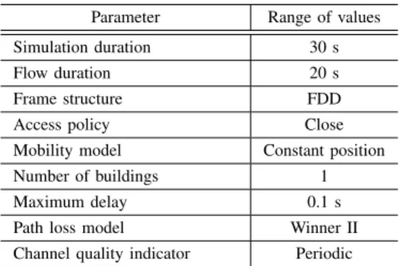
TABLE II
CONSIDERED SIMULATION PARAMETERS.
Parameter Range of values Simulation duration 30 s
Flow duration 20 s
Frame structure FDD
Access policy Close
Mobility model Constant position
Number of buildings 1
Maximum delay 0.1 s
Path loss model Winner II Channel quality indicator Periodic
Two applications are simultaneously used. One is the video application, a video trace that is compressed using the H.264 standard compression at the average coding rate of 440 kb/s. More details are given in [19]. The adoption of this video application accounts for the trend of users to watch high quality videos. The other application is best effort (BE). These BE flows are modelled through infinite buffer sources which model an ideal source where there are always packets to be sent. We evaluate the network performance by considering these video and BE flows [19].
In the simulations, we assume that the eNB 20 MHz bandwidth is split into two equal parts to be made available to the HeNBS, each portion with 10 MHz bandwidth. The four HeNB are placed as shown in Fig. 1. The network performance has been evaluated with reference to the goodput achieved by BE flows and the goodput, packet loss ratio (PLR) and delay of video.
B. Results with PF
Fig. 3 presents the average goodput with the use of the PF scheduler for video application.
Tx. P ower [dBm] −10 −5 0 5 10 15 20 Side [m] 5 10 15 20 Avg. Goodput [Mb/s] 6.0 6.5 7.0 ● ● ● ● ● ● ● ● ● ● ● ● ● ● ● ● ● ● ● ● ● ● ● ● ● ● ● ●
Fig. 3. Variation of the average goodput of video flows, with PF scheduler for different values of transmitter power and apartment side. The fitting was made using a polynomial surface with 95% confidence interval.
The maximum values for the average goodput have been obtained when the apartment side is 5 m and the transmitter power is 20 dBm. The lowest values have been obtained when the apartment side is 20 m and the transmitter power is -10 dBm. For BE flows, in Fig. 4 the maximum and minimum values for the goodput have been obtained in the same points as for the video flows in Fig. 3. For both flows, the obtained results are in line with the results obtained for the average SINR. Tx. P ower [dBm] −10 −5 0 5 10 15 20 Side [m] 5 10 15 20 A vg. Goodput [Mb/s] 30 35 40 45 50 ● ● ● ● ● ● ● ● ● ● ● ● ● ● ● ● ● ● ● ● ● ● ● ● ● ● ● ●
Fig. 4. Variation of the average goodput of BE flows, with PF scheduler and for different values of transmitter power and apartment side. The fitting was made using a polynomial surface with 95% confidence interval.
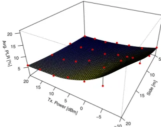
The average packet loss ratio for video flows, shown in Fig. 5, presents values that go beyond the maximum of 2% indicated by the 3GPP. However, it is possible to obtain results for the PLR lower than or closer to 2%, namely when the apartment side is 5 m For transmitter power of 5 dBm and
apartment side of 5 m, the PLR is 2%. For larger apartment sides the PLR is higher than 2%.
Tx. P ower [dBm] −10 −5 0 5 10 15 20 Side [m] 5 10 15 20 Avg. PLR [%] 5 10 15 20 ● ● ● ● ● ● ● ● ● ● ● ● ● ● ● ● ● ● ● ● ● ● ● ● ● ● ● ●
Fig. 5. Variation of the average packet loss ratio of video flows, with PF scheduler and for different values of transmitter power and apartment side. The fitting was made using a polynomial surface with 95% confidence interval.
With any of the considered schedulers, the 3GPP limit of 150 ms for the maximum delay has not been overcame. C. Results with FLS
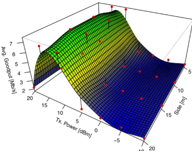
Comparing the average goodput of video flows with the use of the FLS scheduler, as shown in Fig. 6, with the previous case (PF scheduler), shown in Fig. 3, with the FLS scheduler, the average goodupt increases, although both schedulers have identical behaviour . Tx. P ower [dBm] −10 −5 0 5 10 15 20 Side [m] 5 10 15 20 Avg. Goodput [Mb/s] 6.7 6.8 6.9 7.0 7.1 7.2 ● ● ● ● ● ● ● ● ● ● ● ● ● ● ● ● ● ● ● ● ● ● ● ● ● ● ● ●
Fig. 6. Variation of the average goodput of video flows, with FLS scheduler for different values of transmitter power and apartment side. The fitting was made using a polynomial surface with 95% confidence interval.
When the transmitter power is 20 dBm and the apartment side is 20 m, the average goodput clearly increases by a value near 0.45 Mb/s, from 6.83 Mb/s to 7.27 Mb/s. Even in the worst case, for a transmitter power of -10 dBm and apartment side of 20 m, the average goodput increases more than 1.2 Mb/s, from 5.47 Mb/s to 6.73 Mb/s. Since video takes advantage form the FLS scheduler, the BE application is penalized. The average goodput for the BE application,
as shown in Fig. 7, is in average, circa 1 Mb/s lower than the previous case Fig. 4. The adoption of the FLS scheduler
Tx. P ower [dBm] −10 −5 0 5 10 15 20 Side [m] 5 10 15 20 A vg. Goodput [Mb/s] 30 35 40 45 ● ● ● ● ● ● ● ● ● ● ● ● ● ● ● ● ● ● ● ● ● ● ● ● ● ● ● ●
Fig. 7. Variation of the average goodput of BE flows, with FLS scheduler and for different values of transmitter power and apartment side. The fitting was made using a polynomial surface with 95% confidence interval.
also brings advantages in the results obtained for the PLR for the video application, as shown in Fig. 8. By comparing
Tx. P ower [dBm] −10 −5 0 5 10 15 20 Side [m] 5 10 15 20 Avg. PLR [%] 2 4 6 8 ● ● ● ● ● ● ● ● ● ● ● ● ● ● ● ● ● ● ● ● ● ● ● ● ● ● ● ●
Fig. 8. Variation of the average packet loss ratio of video flows, with FLS scheduler and for different values of transmitter power and apartment side. The fitting was made using a polynomial surface with 95% confidence interval.
these results with the values obtained for the PF scheduler, as shown in Fig. 5, the average PLR with the FLS decays, and it is possible to keep the PLR lower than 2% for more combinations of the transmitter power and apartment side. Even the worst values obtained decay from a maximum of 23.4% to a maximum of 7.6%. Both values were obtained for the same transmitter power of -10 dBm and apartment side of 20 m.
D. Results with EXPRule
Contrary to the previous cases, Fig. 3 and Fig. 6, the behaviour of the average goodput of video flows with the use of the EXPRule scheduler is more irregular, as shown in Fig. 9, and has a clear local maximum.
The maximum average values of the goodput for the video application occurs for transmitter powers between 10 and
Tx. P ower [dBm] −10 −5 0 5 10 15 20 Side [m] 5 10 15 20 Avg. Goodput [Mb/s] 2 3 4 5 6 7 ● ● ● ● ● ● ● ● ● ● ● ● ● ● ● ● ● ● ● ● ● ● ● ● ● ● ● ●
Fig. 9. Variation of the average goodput of video flows, with EXPRule scheduler for different values of transmitter power and apartment side. The fitting was made using a polynomial surface with 95% confidence interval.
15 dBm. By considering a constant transmitter power, the variation of the size of the apartment does not impact the average goodput. Although the maximum average goodput is identical in the three schedulers, the EXPRule scheduler present the worst average goodput for the video application. Since the video flows were impaired by the use of the BE flows, the average goodput for the BE flows increases, as shown in Fig 10. Tx. P ower [dBm] −10 −5 0 5 10 15 20 Side [m] 5 10 15 20 A vg. Goodput [Mb/s] 35 40 45 50 ● ● ● ● ● ● ● ● ● ● ● ● ● ● ● ● ● ● ● ● ● ● ● ● ● ● ● ●
Fig. 10. Variation of the average goodput of BE flows, with EXPRule scheduler and for different values of transmitter power and apartment side. The fitting was made using a polynomial surface with 95% confidence interval.
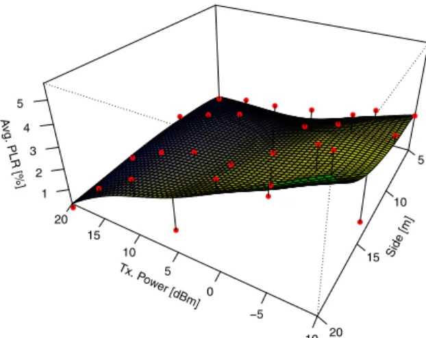
As an example, the average goodput with the EXPRule scheduler is 6 Mb/s higher than the average goodput for BE flows, as shown in Fig. 7. Although the EXPRule scheduler is not itself the best choice in terms of goodput, the average PLR for video flows, for values of transmitter power equal or higher than 0 dBm, is in most of the cases lower than 2%, as shown in Fig 11. In fact, the maximum PLR is the lowest from the three studied schedulers, with a value of 6.4%.
IV. CONCLUSIONS
Seeking the reduction of energy consumption is one of the main priorities in future telecommunications systems. In this
Tx. P ower [dBm] −10 −5 0 5 10 15 20 Side [m] 5 10 15 20 A vg. PLR [%] 1 2 3 4 5 ● ● ● ● ● ● ● ● ● ● ● ● ● ● ● ● ● ● ● ● ● ● ● ● ● ● ● ●
Fig. 11. Variation of the average packet loss ratio of video flows, with EX-PRule scheduler and for different values of transmitter power and apartment side. The fitting was made using a polynomial surface with 95% confidence interval.
work the analytical behaviour of the system is investigated with a study of the average SINR and the performance of the PF, FLS and EXPRule schedulers. The approach considered only four HeNBs (also know as Enterprise HeNBs), each of them serving 8 users.
The study of the average SINR has shown that, for values of the transmitter power between 0 and 20 dBm, the average SINR did not vary for the same apartment side. The average SINR study has shown that the smaller the radius is, the higher the average SINR values are achievable. For values of the transmitter power between -10 and 0 dBm the average SINR decays faster, specially for apartment sides longer than 8 m.
Performance evaluation considered LTE-Sim. The PF and FLS schedulers perform in a very identical way in terms of average goodput, with a slight advantage for the FLS. However, in terms of the average PLR, the FLS presents better performance, since it achieves values lower than 2% more often. This performance enhancement occurs when the transmitter power is between 10 and 20 dBm for all the apartment sides. In this comparison between the PF scheduler and the FLS, the PF scheduler also presents better results for the average goodput for BE flows. This two schedulers confirm the expected results for average SINR that were analytically derived.
Contrary to the PF scheduler and FLS, the best performance of EXPRule scheduler was obtained for transmitter powers be-tween 10 and 15 dBm. It is important to note that the values of average goodput for video flows are identical for a transmitter power of either 20 dBm or 0 dBm. For the average PLR, values lower than 2% were achieved for transmitter power lower than 15 dBm when the apartment side is 20 m. But when the apartment side is 5 m, values of average PLR lower than 2% were obtained for values of the transmitter power higher than 5 dBm. With EXPRule scheduler, the variation of the average goodput of BE flows, shows a behaviour approximated to the one from other studied schedulers.
It is important to highlight that is possible to operate the
system without the need to set the HeNBs transmitter power to the maximum value without compromising the overall system performance. If the transmitter power is set to lower values this can be a step to achieve greener mobile communication systems.
REFERENCES
[1] J. Andrews, H. Claussen, M. Dohler, S. Rangan, and M. Reed, “Fem-tocells: Past, present, and future,” Selected Areas in Communications, IEEE Journal on, vol. 30, no. 3, pp. 497–508, April 2012.
[2] I. Ashraf, H. Claussen, and L. T. W. Ho, “Distributed radio coverage op-timization in enterprise femtocell networks,” in 2010 IEEE International Conference on Communications, May 2010, pp. 1–6.
[3] S. R. Valizadeh and J. Abouei, “An adaptive distributed coverage optimization scheme in LTE enterprise femtocells,” in 2014 22nd Iranian Conference on Electrical Engineering (ICEE), May 2014, pp. 1723– 1728.
[4] Cisco and/or its affiliates, “Cisco visual networking index: Forecast and methodology, 2016–2021,” July 2017. [Online]. Available: https://www.cisco.com/c/en/us/solutions/collateral/service- provider/visual-networking-index-vni/complete-white-paper-c11-481360.pdf
[5] J. Wu, B. Cheng, M. Wang, and J. Chen, “Energy-efficient bandwidth aggregation for delay-constrained video over heterogeneous wireless networks,” IEEE Journal on Selected Areas in Communications, vol. 35, no. 1, pp. 30–49, Jan 2017.
[6] J. Wu, C. Yuen, B. Cheng, M. Wang, and J. Chen, “Energy-minimized multipath video transport to mobile devices in heterogeneous wireless networks,” IEEE Journal on Selected Areas in Communications, vol. 34, no. 5, pp. 1160–1178, May 2016.
[7] S. Sesia, I. Toufik, and M. Baker, LTE, The UMTS Long Term Evolution: From Theory to Practice, 2nd Edition. Wiley Publishing, 2011. [8] T. S. Rappaport, Wireless Communications: Principles and Practice,
2nd ed. Upper Saddle River, NJ: Prentice Hall PTR, 2002.
[9] H. Holma and A. Toskala, WCDMA for UMTS - HSPA evolution and LTE, 1st ed. West Sussex, England: JohnWiley & Sons, Ltd., 2007. [10] K. Chen and J. de Marca, Mobile WiMAX, ser.
Wiley - IEEE. Wiley, 2008. [Online]. Available: https://books.google.es/books?id=7TWzvbZkLMgC
[11] P. Kyösti, J. Meinilä, L. Hentilä, X. Zhao, T. Jämsä, C. Schneider, M. Narandzic, M. Milojevic, A. Hong, J. Ylitalo, and V.-M. Holappa, “IST-4-027756 WINNER II d1.1.2 v1.2 WINNER II channel models,” Tech. Rep., February 2008. [Online]. Available: http://www.cept.org/files/1050/documents/winner2 - final report.pdf [12] G. Piro, L. Grieco, G. Boggia, F. Capozzi, and P. Camarda, “Simulating
LTE cellular systems: An open-source framework,” Vehicular Technol-ogy, IEEE Transactions on, vol. 60, no. 2, pp. 498–513, Feb 2011. [13] R. Basukala, H. Mohd Ramli, and K. Sandrasegaran, “Performance
analysis of EXP/PF and M-LWDF in downlink 3GPP LTE system,” in Internet, 2009. AH-ICI 2009. First Asian Himalayas International Conference on, Nov 2009, pp. 1–5.
[14] G. Piro, L. Grieco, G. Boggia, R. Fortuna, and P. Camarda, “Two-level downlink scheduling for real-time multimedia services in LTE networks,” Multimedia, IEEE Transactions on, vol. 13, no. 5, pp. 1052– 1065, Oct 2011.
[15] E. Dahlman, S. Parkvall, J. Skold, and P. Beming, 3G Evolution, Second Edition: HSPA and LTE for Mobile Broadband, 2nd ed. Academic Press, 2008.
[16] S. Shakkottai and A. L. Stolyar, “Scheduling for multiple flows sharing a time-varying channel: The Exponential Rule,” American Mathematical Society Translations, Series, vol. 2, p. 2002, 2000.
[17] B. Sadiq, S. J. Baek, and G. de Veciana, “Delay-optimal opportunistic scheduling and approximations: The Log Rule,” Networking, IEEE/ACM Transactions on, vol. 19, no. 2, pp. 405–418, April 2011.
[18] G. TSG-RAN4#51, Alcatel-Lucent, picoChip Designs, and Vodafone, “R4-092042, simulation assumptions and parameters for FDD HeNB RF requirements,” May 2009.
[19] F. Capozzi, G. Piro, L. Grieco, G. Boggia, and P. Camarda, “On accurate simulations of LTE femtocells using an open source simulator,” EURASIP Journal on Wireless Communications and Networking, vol. 2012, no. 1, p. 328, 2012. [Online]. Available: http://jwcn.eurasipjournals.com/content/2012/1/328