Analysis of the anatomical and functional basis of autism spectrum conditions using magnetic resonance imaging and electroencephalography

(1)

UNIVERSIDADE DE LISBOA

Analysis of the Anatomical and F

basis of Autism Spectrum C

Magnetic Resonance Imaging and

Electroencephalography

Ana Maria Ferreira Paradela Catarino

DOUTORAMENTO EM

UNIVERSIDADE DE LISBOA

F

ACULDADE DE

C

IÊNCIAS

Departamento de Física

Analysis of the Anatomical and Functional

Autism Spectrum Conditions

Magnetic Resonance Imaging and

lectroencephalography

Ana Maria Ferreira Paradela Catarino

OUTORAMENTO EM ENGENHARIA BIOMÉDICA E BIOFÍSICA 2012

unctional

onditions using

Magnetic Resonance Imaging and

(2)

(3)

UNIVERSIDADE DE LISBOA

Analysis of the Anatomical and Functional

basis of Autism Spectrum Conditions

Magnetic Resonance Imaging and

Electroencephalography

Ana Maria Ferreira Paradela Catarino

Instituto de Biofísica e Engenharia Biomé Faculdade de Ciê

DOUTORAME

UNIVERSIDADE DE LISBOA

F

ACULDADE DE

C

IÊNCIAS

Departamento de Física

Analysis of the Anatomical and Functional

basis of Autism Spectrum Conditions

Magnetic Resonance Imaging and

Electroencephalography

Ana Maria Ferreira Paradela Catarino

Thesis supervised by:

Professor Doutor Alexandre Andrade Instituto de Biofísica e Engenharia Biomédica Faculdade de Ciências, Universidade de Lisboa

OUTORAMENTO EM ENGENHARIA BIOMÉDICA E BIOFÍSICA 2012

Analysis of the Anatomical and Functional

basis of Autism Spectrum Conditions using

(4)

(5)

(6)

i

4.2. METHODS ... 68 4.2.1. PARTICIPANTS ... 68 4.2.2. EEG RECORDING ... 69 4.2.3. SIGNAL ANALYSIS ... 70 4.2.4. MULTISCALE ENTROPY... 71 4.2.5. POWER ANALYSIS ... 72 4.2.6. STATISTICAL ANALYSIS ... 73 4.3. RESULTS ... 74 4.3.1. BEHAVIOURAL PERFORMANCE ... 74 4.3.2. MSE ANALYSIS ... 74 4.3.3. POWER ANALYSIS ... 78 4.4. DISCUSSION ... 78

5. INTERHEMISPHERIC FUNCTIONAL CONNECTIVITY IN AUTISM SPECTRUM CONDITIONS:AN EEG STUDY USING WAVELET COHERENCE TRANSFORM ... 83

5.1. INTRODUCTION ... 83

5.1.1. COHERENCE AND CONNECTIVITY ... 83

5.1.2. COHERENCE AND CONNECTIVITY IN ASC ... 84

(9)

iv

5.2. METHODS ... 86

5.2.1. PARTICIPANTS ... 86

5.2.2. EEG RECORDING ... 87

5.2.3. SIGNAL ANALYSIS ... 87

5.2.4. WAVELET TRANSFORM COHERENCE ... 88

5.2.5. STATISTICAL ANALYSIS ... 91 5.3. RESULTS ... 92 5.3.1. BEHAVIOURAL PERFORMANCE ... 92 5.3.2. WTC ANALYSIS ... 92 5.4. DISCUSSION ... 100 6. GENERAL DISCUSSION ... 107

6.1. UNIFYING MODELS OF ASC ... 107

6.1.1. ATYPICAL NEURAL CONNECTIVITY IN ASC ... 108

6.1.2. LIMITATIONS OF THE DATASETS USED IN THIS THESIS ... 109

6.2. fMRI MEASURES OF CONNECTIVITY IN ASC ... 110

6.2.1. LIMITATIONS ON THE INTERPRETATION OF THE fMRI STUDY DESCRIBED IN CHAPTER 3 .... 112

6.3. EEG MEASURES OF CONNECTIVITY IN ASC ... 112

6.4. ANATOMICAL MEASURES OF CONNECTIVITY IN ASC ... 114

6.5. LIMITATIONS OF THE CONNECTIVITY THEORY IN ASC AND FUTURE PERSPECTIVES ... 115

6.6. CONCLUSIONS ... 116

(10)

v

LIST OF FIGURES

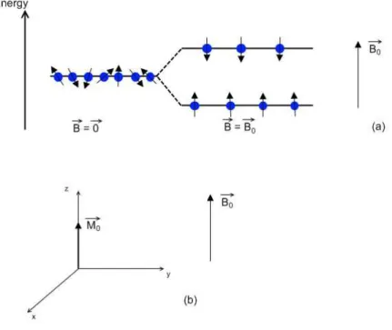
Figure 1.1 – The protons’ magnetic moments align parallel or anti-parallel in the presence of

an external field (a) and differences in energy states generate a positive net magnetization, in

the same direction as the main field (b). ... 5

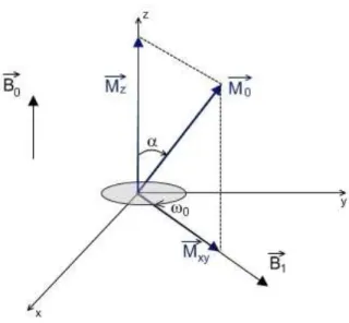
Figure 1.2 – When an RF pulse is applied, the net magnetization is flipped by an angle α. . 6

Figure 1.3 – The rotating frame of reference, rotating at the Larmor frequency; the RF magnetic pulse and magnetization vector will appear to be stationary. ... 6

Figure 1.4 – Transverse magnetization decay, due to spin-spin interactions. ... 7

Figure 1.5 – Decay of transverse magnetization Mxy due to spin-spin interactions and field inhomogeneities. ... 8

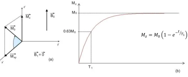
Figure 1.6 – Recovery of longitudinal magnetization Mz due to spin-lattice interactions. ... 8

Figure 1.7 – (a) T1-weighted image of the brain, showing cerebrospinal fluid in dark, brain matter in mid-gray and adipose (fat) tissue in bright tones; (b) T2-weighted image of the brain showing cerebrospinal fluid as very bright and brain and other types of tissue in mid-gray. ... 9

Figure 1.8 – Gradient echo sequence ... 10

Figure 1.9 - Spin echo sequence ... 11

Figure 1.10 – Gradients in the x, y and z axis are used for spatial encoding; ... 13

Figure 1.11 – Spin-echo (SE) imaging sequence ... 14

Figure 1.12 – Gradient echo based echo planar imaging (GE-EPI) sequence ... 15

Figure 1.13 – Blood Oxygen Level Dependent (BOLD) response to neural activity. ... 16

Figure 1.14 – Diagram of brain anatomy showing the corpus callosum, cerebral cortex, brain stem and cerebellum, as well as the functionally segregated lobes. ... 19

Figure 1.15 – Diagram of a neuron’s resting potential. ... 19

Figure 1.16 – Neuron’s structure and stimulus propagation diagram ... 20

Figure 1.17 – Action potential being generated and propagated along the axon of a neuron (a) and a diagram illustrating a referential montage (b). ... 21

Figure 1.18 – Placement of electrodes on the scalp according to the International 10-20 system. ... 22

Figure 1.19 – Example of an EEG power graph. ... 25

Figure 1.20 – Averaging procedure in EEG data to extract ERP waveform. ... 26

Figure 2.1 – Boxplot representations of the age distribution for both Control and ASC groups. ... 37

(11)

vi

Figure 2.2 – Variation of cortical thickness results with kernel width. ... 38 Figure 2.3 – Group differences in cortical thickness for kernel width of FWHM = 10 mm. ... 39 Figure 2.4 – Group differences in cortical thickness-age correlation for kernel width of FWHM =

10 mm. ... 40

Figure 3.1 – Example of 1st level analysis modelation of experimental conditions ... 51 Figure 3.2 – T-maps of increased brain activity to Incongruent compared to Congruent stimuli

(Concrete sentences only) in left (LH) and right (RH) hemispheres, for selected axial slices, for Control (A) and ASC (B) participants, at pFDR-corr < 0.05 (cluster level) ... 54

Figure 3.3 – T-maps of increased brain activity for Congruent relative to Incongruent stimuli

(Emotional sentences only) in left (LH) and right (RH) hemispheres, for selected axial slices, for Controls, at pFDR-corr < 0.05 (cluster level). ... 56

Figure 4.1 – Example of stimuli sequence shown to participants, for both face and chair tasks

... 70

Figure 4.2 - Schematic illustration of the coarse-graining procedure ... 72 Figure 4.3 - Sample entropy by scale factor (SF) graphs for the chairs task, for each electrode,

for each group ... 75

Figure 4.4 - Sample entropy by scale factor (SF) graphs for the faces task, for each electrode,

for each group ... 75

Figure 4.5 - Sample entropy by scale factor (SF) graphs for electrode T7, for both chairs and

faces task. ... 76

Figure 4.6 – Electrodes that presented a significant group-by-scale factor (SF) interaction ... 78 Figure 5.1 – Statistical group comparison of interhemispheric coherence for the chairs task, not

corrected for multiple comparisons ... 94

Figure 5.2 – Statistical group comparison of interhemispheric coherence for the faces task, not

Figure 5.3 – Statistical group comparison of interhemispheric coherence, corrected for

multiple comparisons using the False Discovery Rate (FDR) algorithm ... 97

Figure 5.4 - Statistical task comparison of interhemispheric coherence for the ASC group, not

Figure 5.5 - Statistical task comparison of interhemispheric coherence for the Control group,

(12)

vii

LIST OF TABLES

Table 2.1 - Age, verbal IQ, performance IQ and full-scale IQ for each group ... 33

Table 2.2 - Diagnosis criteria for participants in the ASC group ... 35

Table 3.2 - Response times for each group and each sentence type ... 52

Table 3.3 - Accuracy scores for each group and each sentence type ... 53

Table 3.4 - T, Z, p FDR-corrected and uncorrected values for voxels and clusters activated more in response to Concrete Incongruent stimuli than to Concrete Congruent stimuli, for each group ... 55

Table 3.5 - T, Z, p FDR-corrected and uncorrected values for voxels and clusters activated more in response to Emotional Congruent stimuli than to Emotional Incongruent stimuli, for the Control group ... 57

Table 4.2 - Accuracy (out of 10) and response times (in ms) for both tasks, for each group ... 74

Table 4.3 - Group-by-scale factor (SF) interaction significance values for each electrode site .. 77

Table 6.1 - Summary of methods and results of the different studies performed in the context of this thesis ... 117

(13)

(14)

ix

LIST OF ABBREVIATIONS

ADI-R – Autism Diagnostic Interview - Revised ADOS – Autism Diagnostic Observation Schedule ANOVA – Analysis of Variance

AQ – Autism Quotient

ASC – Autism Spectrum Conditions BA – Brodmann Area

BOLD – Blood Oxygenation Level Dependent CC – Concrete Congruent

CI – Concrete Incongruent CSF – Cerebrospinal Fluid DTI – Diffusion Tensor Imaging EC – Emotional Congruent EEG - Electroencephalography EI – Emotional incongruent EPI – Echo Planar Imaging ERC – Event Related Coherence ERP – Event Related Potential FDR – False Discovery Rate FFA – Fusiform Face Area FFT – Fast Fourier Transform

fMRI – functional Magnetic Resonance Imaging FSIQ – Full Scale Intelligence Quotient

FWHM – Full Width at Half Maximum GE-EPI – Gradient Echo Echo Planar Imaging HFA – High Functioning Autism

ICA – Independent Component Analysis IQ – Intelligence Quotient

LH – Left Hemisphere

MEG - Magnetoecephalography MNI – Montreal Neurological Institute

(15)

x MRI – Magnetic Resonance Imaging

MSE – Multiscale Entropy

PCA – Principal Component Analysis PET – Positron Emission Tomography PIQ – Performance Intelligence Quotient RF - Radiofrequency

RH – Right Hemisphere SD – Standard Deviation SE – Spin Echo

SF – Scale Factor

STS – Superior Temporal Sulcus TE – Echo time

TR – Repetition time

VIQ – Verbal Intelligence Quotient

WASI – Wechsler Abbreviated Scale of Intelligence WTC – Wavelet Transform Coherence

(16)

xi

ABSTRACT

Autism Spectrum Conditions (ASC) are a set of pervasive neurodevelopmental conditions defined by a triad of impairments in social interaction, communications and behavioural flexibility. Previous investigations have provided a variety of evidence of neuroanatomical and neurofunctional impairments in people with ASC, and several explanatory models for ASC have been proposed. One of the most commonly cited is the connectivity model, proposing that ASC symptoms are caused by patterns of atypical neural connectivity.

In this thesis, different algorithms were employed for the analysis of neuroanatomical and neurofunctional data acquired from people with ASC and typically developing controls. Regarding anatomy, a cortical thickness analysis was performed, using magnetic resonance imaging (MRI) data. Although differences were found between controls and ASC patients, the results were inconsistent with previous literature and did not support the connectivity model under consideration.

The findings of the functional analyses however, directly or indirectly support the connectivity model of ASC. A functional MRI (fMRI) investigation of neural activation in response to written sentences showed that people with ASC activate mainly frontal areas, whilst the Control group activates areas over all regions of the cortex. These differences indirectly suggest patterns of reduced connectivity in ASC. A multiscale entropy (MSE) analysis of electroencephalographic (EEG) data acquired during performance of a visual discrimination task demonstrated patterns of decreased EEG complexity for the ASC group relative to the Control group. This also indirectly supports the model of reduced connectivity in ASC. Finally, a wavelet transform coherence (WTC) analysis of the same EEG data set showed decreased interhemispheric EEG coherence for the ASC group relative to the Control group, providing direct evidence supporting the connectivity model of ASC.

Overall, this thesis presents a set of results congruent with the connectivity model of ASC, highlighting the importance of unification of results in ASC research.

Keywords: Autism Spectrum Conditions, connectivity model, magnetic resonance imaging,

(17)

(18)

xiii

RESUMO

As desordens do espectro do autismo (DEA) são um conjunto de condições caracterizadas por uma disfunção global do desenvolvimento neurológico, que se manifesta na infância e cujos sintomas se prolongam por toda a vida adulta. Estudos estatísticos demonstram que as DEA afectam 6 em cada 1000 indivíduos, com uma incidência maior no sexo masculino em relação ao sexo feminino (4:1). Em termos sintomatológicos, as DEA são definidas por um conjunto de disfunções na interacção social e na comunicação, desde ausência completa de desenvolvimento de linguagem a alterações subtis da semântica e pragmática. Estas desordens são também caracterizadas pela presença de padrões de comportamentos rígidos e repetitivos. Este conjunto de sintomas aponta para uma disfunção global da função cerebral em indivíduos com DEA, e inúmeras investigações têm sido realizadas na tentativa de revelar as bases neuroanatómicas e neurofuncionais das DEA. No entanto, a maior parte destas investigações consiste em estudos com pequenas amostras de população, focados em aspectos sintomatológicos específicos, o que muitas vezes resulta em investigações com resultados inconsistentes ou contraditórios entre si.

A unificação de resultados de investigações neuroanatómicas e neurofuncionais, mas também bioquímicas e genéticas, é essencial para uma melhor caracterização das DEA e consequentemente para uma melhoria nas estratégias para o tratamento e prevenção das DEA. Vários modelos de unificação para as DEA têm sido propostos nas últimas décadas, sendo que um dos modelos mais abrangentes, e presentemente um dos mais citados, é o modelo da conectividade neuronal atípica em DEA. Este modelo defende que os sintomas e comportamentos que caracterizam as DEA são o resultado de uma disfunção global da conectividade neuronal (em particular um défice de conectividade neuronal de longo alcance) em indivíduos com DEA.

O objectivo desta tese era realizar uma análise do substrato neuroanatómico e neurofuncional das DEA, utilizando dados de resonância magnética (MRI do inglês Magnetic Resonance

Imaging) e electroencefalografia (EEG), adquiridos em duas populações – um grupo de

indivíduos com DEA e um grupo de indivíduos normais (grupo de controlo).

Relativamente ao aspecto neuroanatómico, foi efectuada uma análise de espessura cortical em imagens estruturais adquiridas por MRI. Estas imagens foram adquiridas de um grupo de 11 indivíduos com DEA e um grupo de 13 indivíduos normais. Todos os indivíduos eram do

(19)

xiv

sexo masculino, não havendo diferença de idade ou QI (quociente de inteligência) médio entre os dois grupos (Idade: DEA: 27 anos, Controlo: 34 anos, F1, 23 = 2.042, P = 0.167; QI: DEA: 115, Controlo: 121, F1, 17 = 1.042, P = 0.323). As imagens de MRI foram adquiridas no Wolfson Brain Imaging Centre, Universidade de Cambridge, num scanner SIEMENS MAGNETOM TrioTim de 3 Tesla, com uma resolução espacial de 1.0 mm. A análise de espessura cortical foi efectuada utilizando o software Freesurfer, enquanto que as comparações estatísticas entre grupos foram efectuadas utilizando o software SPSS v17.0. Os resultados da análise de espessura cortical mostram diversas regiões onde o grupo com DEA apresenta um aumento ou uma diminuição de espessura cortical relativamente ao grupo de Controlo. Regiões de aumento relativo de espessura cortical incluem o lobo frontal médio esquerdo, lobos parietais superiores e inferiores, bem como a circunvolução orbitofrontal medial direita. Regiões de diminuição relativa de espessura cortical incluem o lobo frontal superior esquerdo, lobos temporais superiores e sulcos pré-centrais. No entanto, estes resultados não são consistentes com os resultados de investigações anteriores de espessura cortical em DEA. Isto pode dever-se a diversos factores, como variações nos algoritmos utilizados em cada investigação para o cálculo de espessura cortical. Ainda assim, esta inconsistência de resultados, aliada a outros factores como um largo espectro de idades da população em estudo (16 a 57 anos), sugere que neste caso os resultados da análise são inconclusivos, não sendo possível estabelecer uma relação entre espessura cortical e sintomatologia em DEA.

Pelo contrário, os resultados de todas as análises neurofuncionais efectuadas no contexto desta tese apoiam directa ou indirectamente o modelo da conectividade atípica em DEA. Em primeiro lugar, foi realizada uma análise da activação neuronal em resposta a incongruências semânticas, utilizando dados de resonância magnética funcional (fMRI) adquiridos num grupo de 12 indivíduos com DEA e 12 indivíduos normais. Como se verificou para o estudo neuranatómico, não foram detectadas diferenças de idade ou de QI entre os dois grupos (Idade: DEA: 27 anos, Controlo: 34 anos, F1, 23 = 2.433, P = 0.133; QI: DEA: 113, Controlo: 120, F1, 17 = 1.086, P = 0.313). As imagens de fMRI foram adquiridas no Wolfson Brain Imaging Centre, Universidade de Cambridge, com uma resolução espacial de 3.0 x 3.0 x 4.0 mm. Durante a aquisição de imagens, pediu-se aos indivíduos para lerem um conjunto de frases e decidirem se para cada frase, a palavra final era semanticamente congruente ou incongruente. As frases foram apresentadas visualmente, uma palavra de cada vez, e estavam divididas em quatro categorias – concreta congruente (e.g.: The car had a flat tyre), concreta incongruente (e.g.: The fountain pen leaked blue chocolate), emocional congruente (e.g.: The snake hissed and he felt scared) e emocional incongruente (e.g.: The scientists predicted an epidemic and

(20)

xv

she felt hungry). A análise das imagens de fMRI foi feita utilizando o software SPM5, e os resultados demonstram que, em resposta a frases incongruentes, os indivíduos com DEA activaram maioritariamente regiões frontais (em particular o lobo temporal inferior esquerdo), enquanto que os indivíduos normais activaram uma maior variedade de regiões corticais, incluindo córtices cingulados anterior e posterior, e lobo occipitotemporal. Estas diferenças entre grupos na extensão da activação neuronal apontam indirectamente para a existência de um défice de conectividade neuronal em DEA.

Duas análises funcionais foram também efectuadas utilizando dados de EEG. Estes dados foram adquiridos num grupo de 15 indivíduos com DEA e 15 indivíduos normais, durante o processamento visual de imagens de faces e cadeiras. Como se verificou nos estudos de espessura cortical e fMRI, também neste caso não foram detectadas diferenças de idade ou QI entre os dois grupos (Idade: DEA: 31, Controlo: 29, F1, 29 = 0.961, P = 0.335; QI: DEA: 119, Controlo: 119, F1, 28 = 0.007, P = 0.936). Os dados de EEG foram adquiridos no Departamento de Psiquiatria, Universidade de Cambridge, através de um sistema Synamps de 32 canais, com frequência de aquisição de 1000 Hz e um filtro passa-banda entre 0.1 e 50 Hz.

Uma das análises efectuadas consistiu num estudo da complexidade do sinal de EEG, usando um algoritmo de cálculo de entropia em várias escalas – entropia multiescala (MSE do inglês

Multiscale Entropy). Os resultados desta análise mostram uma redução de complexidade do

sinal de EEG para o grupo de indivíduos com DEA relativamente ao grupo de controlo, em particular para regiões parietais e occipitais. A relação entre complexidade de sinais EEG e conectividade neuronal foi já comprovada em investigações prévias, e os resultados desta análise sugerem um défice de conectividade neuronal em indivíduos com DEA, em regiões posteriores do córtex, apoiando indirectamente o modelo de conectividade atípica em DEA. Uma segunda análise efectuada nos dados de EEG pretendia estudar diferenças em coerência interhemisférica entre indivíduos com DEA e indivíduos normais. Esta análise utilizou a técnica de coerência de wavelets (WTC do inglês Wavelet Transform Coherence), um algoritmo cuja principal vantagem é permitir um estudo da variação da coerência em tempo e em frequência, com controlo da resolução temporal e espectral. Os resultados desta investigação demonstram uma redução de coerência inter-hemisférica no grupo com DEA, relativamente ao grupo de controlo, em todas as regiões corticais estudadas (frontal, temporal, parietal e occipital). Estudos prévios já demonstraram a existência de uma correlação entre coerência de sinais EEG e conectividade neuronal, e pode-se concluir que os resultados desta análise mostram um

(21)

xvi

défice de conectividade neuronal inter-hemisférica em DEA, apoiando directamente o modelo da conectividade atípica em DEA.

Esta tese apresenta um conjunto de análises que empregam algoritmos diversos para o estudo da anatomia e função cerebral em DEA. Os resultados destas análises apontam consistentemente para a existência de um distúrbio da conectividade neuronal em indivíduos com DEA, apoiando o modelo da conectividade atípica em DEA. É importante referir que, por conter uma variedade de análises diferentes, esta tese oferece uma perspectiva unificadora na investigação das DEA, salientando a necessidade de estudos de larga escala em DEA, que empreguem diversos níveis de análise (p.ex.: anatómica, funcional), em grandes amostras de população bem caracterizadas em termos demográficos e que incluam indivíduos num largo espectro de idades, desde a infância atá à idade adulta.

Palavras-chave: Desordens do espectro do autismo, modelo de conectividade, ressonância

(22)

xvii

P

UBLICATIONS

Chapter 3 of this thesis has been published as:

Catarino A., Luke L., Waldman S., Andrade A., Fletcher P. C., Ring H. (2011) An fMRI investigation of detection of semantic incongruities in autism spectrum conditions.

European Journal of Neuroscience 33:558-567

Chapter 4 of this thesis has been published as:

Catarino A., Churches O., Baron-Cohen S., Andrade A., Ring H. (2011) Atypical EEG complexity in autism spectrum conditions: a multiscale entropy analysis. Clinical

Neurophysiology 122(12):2375-83

(23)

(24)

xix

ACKNOWLEDGEMENTS

I would like to thank my supervisors, Dr Alexandre Andrade from the Institute of Biophysics and Biomedical Engineering, University of Lisbon, and Dr Howard Ring from the Cambridge Intellectual and Developmental Disabilities Research Group, University of Cambridge. Their helpful advice and prompt availability have contributed greatly to the successful completion of this work.

I would also like to thank all the people who have collaborated in the projects included in this thesis – Dr Lydia Vella and Ms Jennifer Landt for their help with the MRI data acquisition, Dr Paul Fletcher for his help with the MRI data analysis, Dr Owen Churches for the help with the technical aspects of EEG data acquisition and analysis, Professor Simon Baron-Cohen for his support with the EEG projects and Dr Adam Wagner and Dr Peter Watson for their statistical insight. I would also like to thank Professor Eduardo Ducla Soares for introducing me to Biomedical Engineering in the last year of my undergraduate studies, and encouraging me throughout the course of my PhD.

I would like to acknowledge my colleagues at both the Institute of Biophysics and Biomedical Engineering in Lisbon, and the Cambridge Intellectual and Developmental Disabilities Research Group, for all the helpful comments and discussions. Finally I would also like to thank all the admin staff at Cambridge and Beatriz Lampreia in Lisbon, for guiding me through the administrative side of things.

(25)

(26)

1

1.

G

ENERAL

I

NTRODUCTION

1.1. A

UTISM

S

PECTRUM

C

ONDITIONS

Autism Spectrum Conditions (ASC) are a set of pervasive neurodevelopmental conditions with onset in early childhood and a wide range of life-long signs and symptoms. ASC seem to affect boys more frequently than girls, with a male-to-female prevalence rate of 4.3:1. Statistical studies have shown an increase in the prevalence of ASC over the last few decades, from approximately 5 per 10.000 in the 1960’s and 1970’s, to 60 per 10.000 in present times (Newschaffer et al., 2007). The most likely reasons for this increase in prevalence numbers are the evolution of diagnosis methods and historical changes in the criteria for classifying behaviours consistent with ASC phenotype (Newschaffer et al., 2007). Core features of ASC include impairments in reciprocal social interactions, a restricted repetitive range of behaviours, interests and activities, and a variety of language disturbances ranging from complete absence of receptive and expressive speech to subtle disorders of semantics and pragmatics (American Psychiatric Association, 2000). Children with severe ASC often experience a lack or a significant delay in language development. In the latter case, expressive speech is usually characterized by abnormalities such as echolalia, pronoun reversal, production of utterances with no relation to conversational context, aberrant prosody, unresponsiveness to questions and a general lack of drive to communicate (Rapin and Dunn, 2003).

In addition to these characteristic social and cognitive features, atypical patterns of motor functioning and integration are also increasingly recognised as features of ASC. Amongst these are evidence of impaired motor functions (Gidley Larson and Mostofsky, 2006) as well as impaired sensorimotor integration (Haswell et al., 2009) and motor planning and control (Jansiewicz et al., 2006, Rinehart et al., 2006, Freitag et al., 2007). There is evidence that motor deficits may be correlated with the social and cognitive features of ASC (Dziuk et al., 2007), suggesting that motor symptoms may be a core feature of ASC, or a marker for the underlying neurological deficits of this condition.

Sensory functioning has also been recognised as being atypical in people with ASC. In a review by Simmons et al. (2009), the authors have gathered evidence of atypical visual perception in ASC, including perception of biological motion (Kaiser et al., 2010). Driven by the social

(27)

2

impairments presented by people with ASC, many studies have investigated visual face perception and processing in ASC. These studies have reported various abnormalities in face processing in the ASC population, such as atypical patterns of neuronal activation to neutral and emotional face stimuli (Schultz et al., 2000, Harms et al., 2010) and atypical gaze patterns (Kliemann et al., 2010). Past studies on sensory processing have also found evidence of atypical auditory perception (Hitoglou et al., 2010), somatosensory integration (Russo et al., 2010), and reduced adaptability to environmental changes in this population (Russo et al., 2007, Thakkar et al., 2008, Foley Nicpon et al., 2010).

Within ASC, people with Asperger’s syndrome (AS) and high-functioning autism (HFA) share, with those who have more severe autism, deficits in social communication and interaction, sensory and motor functioning, whilst not experiencing the significant language impairment that also characterises severe autism.

However, language is not normal in AS and HFA and the few studies that have examined language function in these cases have reported several disturbances, including difficulties in selecting congruent humorous endings to jokes (Emerich et al., 2003), disturbed narrative skills (Losh and Capps, 2003) and difficulties in arranging sentences coherently and using context to make global inferences (Jolliffe and Baron-Cohen, 2000).

1.1.1. MECHANISM AND CAUSES

The set of signs and symptoms described above seems to suggest an overall impairment of brain function in people with ASC. In attempting to explain the wide range of features that characterise ASC, several models, both functional and anatomical, have been proposed as underlying mechanisms for this generalized disruption in neural performance.

Regarding anatomy post-mortem investigations have found evidence of abnormalities in cortical cytoarchitecture (Casanova and Trippe, 2009, Oblak et al., 2011) and neuronal migration (Korkmaz et al., 2006, Wegiel et al., 2010) in people with ASC. Increased brain volume in early stages of brain development is one of the most often reported findings of in vivo imaging studies in children with ASC (Hardan et al., 2001, Hazlett et al., 2005, Ben Bashat et al., 2007) and it is hypothesized that an overgrowth in white matter may be related with the atypical cytoarchitecture and neuronal migration patterns found in people with ASC

(28)

3

(Courchesne et al., 2005). Other imaging studies of brain structure in adults and children with ASC have found evidence of anatomical abnormalities in the size of specific brain structures such as the corpus callosum (Egaas et al., 1995, Piven et al., 1997) and cerebellum (Scott et al., 2009, Hodge et al., 2010).

Another common finding in brain imaging studies of ASC is altered cortical thickness. However, the direction and location of these changes is not always agreed on, with some studies reporting an increase in total brain cortical thickness in ASC groups, specifically in the temporal lobes (Hardan et al., 2006), and others a decrease in cortical thickness in specific brain regions, namely the right inferior orbital prefrontal cortex, left superior temporal sulcus and left occipito-temporal gyrus (Chung et al., 2005). Two other studies (Hardan et al., 2004, Jou et al., 2010) have also reported patterns of increased cortical gyrification in the frontal lobe of people with ASC, when compared to neurotypical controls.

A correlation between the anatomical abnormalities just described and atypical brain functioning in people is ASC is yet to be established. However, some studies suggest that these structural abnormalities may be reflected in atypical patterns of functional connectivity between neural networks in the autistic brain (Just et al., 2007, Guye et al., 2010). The connectivity model is one of the commonly cited explanatory models of atypical brain functioning in ASC. Since it was introduced by Belmonte et al. (2004b) this model has been investigated and supported by numerous publications (Courchesne and Pierce, 2005b, Just et al., 2007, Monk et al., 2009, Barttfeld et al., 2011, Wass, 2011). Atypical neural connectivity between neural networks leading to disrupted temporal integration of information has also been investigated as an explanatory model for ASC (Brock et al., 2002, Rippon et al., 2007).

The wide range of features and severity of symptoms, along with its high heritability index and high prevalence of co-morbidities with genetic syndromes, makes it likely that the underlying cause for ASC is of genetic nature. The variability of the range and severity of symptoms between individuals with ASC, along with evidence from genetic studies, tells us that ASC is a complex genetic disorder, not caused by a single mutation in a single gene, but by a wide variety of mutations in different sections of the genome (Muhle et al., 2004, Abrahams and Geschwind, 2008). In addition to this, evidence from genetic studies indicates that different atypical genotypes will give rise to different behavioural phenotypes in ASC (Abrahams and Geschwind, 2008). Also of interest is the fact that some studies have found that some genetic mutations thought to be involved in ASC are also involved with other neuropsychiatric

(29)

4

disorders known to occur with increased prevalence in individuals with ASC, such as schizophrenia (Burbach and van der Zwaag, 2009, Carroll and Owen, 2009) and bipolar disorder (Carroll and Owen, 2009). Environmental factors such as toxic exposure (Adams et al., 2007) or prenatal exposure to maternal infection (Atladottir et al., 2010, Landrigan, 2010) have also been reported as possible causes for genetic mutations thought to be involved in ASC.

1.2. M

AGNETIC

R

ESONANCE

I

MAGING

Magnetic resonance imaging (MRI) is a medical imaging technique used to acquire high-resolution images of a certain part of the body. This technique is noninvasive and does not resort to ionizing radiation for image acquisition. Instead, it uses high strength electromagnetic fields to interfere with the magnetic moments of subatomic particles within the body. Different tissues have different magnetic properties, detected by the MRI scanner to form the final image. This section will cover the physical principles behind MRI image acquisition and reconstruction.

1.2.1. PHYSICAL PRINCIPLES

Approximately 75% of the human body is made of water. Protons are elementary particles that are part of water molecules, and are therefore abundant in the human body. Like other charged elementary particles, protons have a characteristic magnetic moment. In the MRI scanner, the main magnetic field causes the protons’ magnetic moments to align either parallel or anti-parallel to (Figure 1.1a). These two states have slightly different energies, with the parallel state having lower energy than the anti-parallel state. For this reason, there is a slight excess of protons in the parallel state, and the sum of all the protons’ magnetic moments generates the net magnetization, , which has the same direction as the main magnetic field (Figure 1.1b).

(30)

5

Due to quantum mechanics laws, the alignment between the protons’ magnetic moments and the external field is not perfect. For this reason, the magnetic moments will precess around the main field’s axis (conventionally the z axis) at a frequency that is dependent on the strength of the magnetic field. This is called the Larmor frequency, and it is given by = , where γ is the gyromagnetic ratio (γ = 2.7x108_rad.s-1_.T-1_{) and B}

0 the strength of the main field, in Tesla. This is the protons’ characteristic frequency, and so the protons will only be affected by electromagnetic waves with the Larmor frequency – this is called the resonance condition. The net magnetization strength is very small compared to the strength of the main field ( ∼ 10 ), and therefore it is very hard to measure the longitudinal net magnetization. However, by applying a radiofrequency (RF) pulse in the Larmor frequency, it is possible to flip the net magnetization, by an angle α, called the flip angle. What the RF pulse does is to create a magnetic field, , perpendicular to , and oscillating at the Larmor frequency around the z axis. The flip angle is given by = , where B1 is the strength of the RF magnetic field and τ is the duration of the RF pulse (Figure 1.2).

Figure 1.1 – The protons’ magnetic moments align parallel or anti-parallel in the presence of an external field (a)

(31)

6

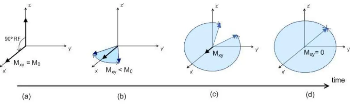
Since the magnetization vector and the RF magnetic pulse are precessing around the vertical z axis at the Larmor frequency, it is easier to consider them in a rotating frame of reference. In a frame ′ ′ ′ rotating around the ≡ axis at the Larmor frequency, and will appear to be stationary (Figure 1.3). If a 90° RF pulse is applied, the flip angle equals 90°. This means that the magnetization vector will be in the transverse ′ ′ plane, so the longitudinal component of the magnetization will be zero, = 0. On the other hand, the transverse magnetization will be maximal, _!= (Figure 1.4a).

Figure 1.2 – When an RF pulse is applied, the net magnetization is flipped by an angle α.

Figure 1.3 – The rotating frame of reference, rotating at the Larmor frequency; the RF magnetic pulse and magnetization vector will appear to be stationary.

(32)

7

As mentioned previously, the net magnetization is the result of the sum of the magnetic moments of all the protons. The magnetic moment of a proton precesses around the axis of the main magnetic field at the Larmor frequency, which depends on the main magnetic field’s strength. However, the protons interact with each other, and are influenced by the magnetic moments of neighbouring protons, which means that each proton experiences a magnetic field that is slightly higher or lower than that of the main magnetic field. Therefore, each proton will precess at a frequency slightly higher or lower than the Larmor frequency. After a 90° RF pulse, this interaction between protons will cause them to become out of phase with each other, and the transverse magnetization will sum up to zero. This dephasing is an exponential decay process known as spin-spin relaxation (Figure 1.4 sequence).

The decay of the strength of the transverse magnetization due to spin-spin relaxation is given by _! = " # $&%, where t is time after the initial RF pulse, and T2 is the spin-spin relaxation time, defined as the time the transverse magnetization signal takes to reach 37% of its original value (Figure 1.5). However, due to various factor including the presence of the patient inside the scanner, the homogeneity of the main field is affected. This leads to an increase in local inhomogeneities in the main field, which in turn accelerates the dephasing of the protons’ magnetic moments and the decay of transverse magnetization. Taking into account spin-spin relaxation and the inhomogeneity of the main field, the decay of strength of the transverse magnetization is given by _!= " #&$%∗, where T2

*_{is a composite relaxation time that} includes T2 and the decay caused by local inhomogeneities in the main field.

(33)

8 ! = " # $_%∗ & ! = " # $&%

Simultaneous to spin-spin decay, after the RF pulse is turned off, the protons’ magnetic moments tend to go back to their equilibrium position, aligned with the main magnetic field (Figure 1.6a). This process occurs through the loss of energy from the protons to the surrounding tissues, or lattice, and is therefore called spin-lattice relaxation. In spin-lattice relaxation, there is a recovery of the longitudinal magnetization given by

= (1 − " # $&*+, where T1 is the spin-lattice relaxation time, defined as the time it takes for the longitudinal magnetization to recover 63% of its original value (Figure 1.6b).

= (1 − " # $&*+

Figure 1.5 – Decay of

transverse magnetization

Mxy due to spin-spin interactions and field inhomogeneities.

(34)

9

Despite the 10-6_{ratio between net magnetization and main field strength, modern MRI} scanners are capable of detecting changes in transverse magnetization and measuring relaxation times T1, T2 and T2

*

by having coils placed orthogonally to the main coil. Due to the fact that different tissues have different molecular compositions, each tissue has its own magnetic properties and consequently its own characteristic relaxation times, which are the basis for image contrast in MRI. T1-weighted images for example, have excellent contrast and are commonly used in anatomical studies. In these images fluids appear dark, water based tissues are mid-gray, and fat based tissues are very bright (Figure 1.7a). On the other hand, in T2-weighted images, fluids are very bright and water and fat based tissues are mid-gray. For this reason, T2-weighted images are commonly used for pathological studies where abnormal collections of fluid appear bright against the darker normal tissue (Figure 1.7b).

1.2.2. ECHOES

In MRI repetitive RF pulses are used to generate echoes of magnetization, whose intensity depends on the relaxation times T2 and T2

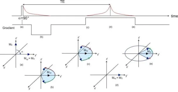
*_{. Different sequences of RF pulses and gradients} generate different types of echoes. There are two main types of echo generating mechanisms used in modern MRI scanners: gradient echo and spin echo.

Gradient echo is generated by an initial RF pulse with a flip angle usually smaller than 90°, followed by a negative gradient in the magnetic field. Spin-spin relaxation and inhomogeneities in the main field cause the protons’ magnetic moments to dephase, leading to a decay in transverse magnetization. A positive gradient in the magnetic field is then applied, compensating for the negative gradient previously described. This will cause the

(a) (b)

Figure 1.7 – (a) T1-weighted image of the brain, showing cerebrospinal fluid in dark, brain matter in mid-gray

and adipose (fat) tissue in bright tones; (b) T2-weighted image of the brain showing cerebrospinal fluid as very bright and brain and other types of tissue in mid-gray. From www.mr-tip.com.

(35)

10

protons’ magnetic moments to rephase, up to the point where all the protons’ magnetic moments are in phase, and transverse magnetization is maximal (Figure 1.8). This is the gradient echo, with intensity given by

,-.= , exp 2−34₃

5∗6 (1.1) Where S0 is the signal intensity (transverse magnetization) after the initial RF pulse, T2

*

is the

spin-spin and field inhomogeneity relaxation time and TE is the gradient echo time, defined as the time it takes for the echo to be formed after the initial RF pulse.

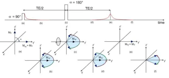
In the spin echo sequence, an initial 90° RF pulse is applied. The protons’ magnetic moments start to dephase and there is decay in the transverse magnetization and signal intensity. A 180° RF pulse is then applied. This will cause the transverse magnetization to flip through 180° about the y’ axis, reversing the phase angles of the protons’ magnetic moments. The precession frequency of the magnetic moments will not change, and the protons will carry on experiencing the same field inhomogeneities as before. This means that after a period of time equivalent to the time gap between the 90° and the 180° RF pulses, the protons’ magnetic moments will rephase and transverse magnetization will be maximal (Figure 1.9). This is called the spin echo, and its intensity is given by

Figure 1.8 – Gradient echo sequence: the initial RF pulse is applied (a), and the negative gradient accelerates the

magnetic moments dephasing and the decay of transverse magnetization (b); when the positive gradient is applied the magnetic moments begin to rephase (c), and there is a moment when all the magnetic moments are in phase again, and an echo is formed (d); the magnetic moments continue their precession around the z axis, and dephase again due to spin-spin interactions (e).

(36)

11

,:. = , exp ;−34₃

5< (1.2) Where S0 is the signal intensity of the transverse magnetization after the initial RF pulse, T2 is the spin-spin relaxation time and TE is the spin echo time, defined as the time it takes for the echo to be formed after the initial 90° RF pulse.

1.2.3. SPATIAL ENCODING

In MRI relaxation and echo times can provide information about the average composition of a given volume. In the human body a volume can be for example the head, with the bone, brain, muscle, fat and cerebrospinal fluid (CSF) as the different types of tissue, each with characteristic relaxation times. Image reconstruction of the tissues within a volume requires a spatial encoding algorithm applied through 3-dimensional magnetic field gradients (variation of strength in the magnetic field with position):

1- A gradient in the z axis direction (same direction as the main magnetic field ) is used for slice selection – Gss; with precessional frequency being directly proportional to field strength, this gradient will cause the protons’ magnetic moment precessional frequency to vary along the main field axis; only magnetic moments precessing at the Larmor frequency will be affected by the RF pulse, and so this gradient will limit the

Figure 1.9 - Spin echo sequence: the initial 90° RF pulse is applied (a), the magnetic moments start to dephase and there is

a decay of transverse magnetization (b); an 180° RF pulse is applied (c) which causes the magnetic moments to begin to rephase (d), and there is a moment when all the magnetic moments are in phase again, and an echo is formed (e); the magnetic moments continue their precession around the z axis, and dephase again due to spin-spin interactions (f).

(37)

12

scope of influence of the RF pulse to a single slice orthogonal to the main field axis (Figure 1.10a)

2- A gradient applied for a limited amount of time, orthogonally to the main field axis, is used for phase encoding – Gpe; this gradient causes a variation in the precessional frequency of the protons’ magnetic moments along the Gpe axis, causing them to dephase; when the gradient is turned off, the magnetic moments will go back to precessing at Larmor frequency, but the difference in phase induced by the phase encoding gradient will be maintained, and magnetic moments on different coordinates along the Gpe axis will have different phases (Figure 1.10b)

3- A gradient applied orthogonally to the slice selection and phase encoding gradients is used for frequency encoding – Gfe; this gradient will cause a variation in the protons magnetic moments’ precessional frequencies along the Gfe axis; the phase and frequency encoding gradients ensure that the protons’ magnetic moments have a characteristic phase and precessional frequency, according to their position in the selected slice; due to these differences in phase and frequency, the echo times will vary depending on the spatial location of the signal source, allowing accurate image reconstruction (Figure 1.10c)

(38)

13

Figure 1.10 – Gradients in the x, y and z axis are used for spatial encoding; after a slice selective gradient

is applied in the same direction as the main magnetic field, a position in the z axis is determined (a); a phase encoding gradient applied orthogonally to the main field axis dephases the magnetic moments according to their position along the phase encoding gradient axis (b); a frequency encoding gradient applied orthogonally to the slice selective and phase encoding gradients makes the precessional frequency vary with the position along the frequency encoding gradient axis (c); at this point each magnetic moment in the selected slice has its own characteristic phase and precessional frequency.

(39)

14

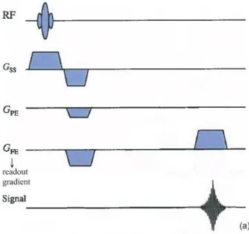
Different types of images can be generated by varying the timings and sequences of these spatial encoding gradients. For most gradient sequences, the frequency encoding gradient is applied last, during the signal reading stage, and for this reason it is usually called the ‘readout gradient’ (Figure 1.11).

Each gradient sequence has their own advantages over others, concerning acquisition time, image resolution and vulnerability to artefacts. For example the gradient echo based echo planar imaging (GE-EPI) (Figure 1.12a) is a fast acquisition sequence, but has the disadvantage of providing low spatial resolution images that are prone to artefacts (Figure 1.12b). This is because in this type of sequence each spatial frequency image space (k-space) is covered in a single repetition time (the time interval between two consecutive RF pulses), limiting the amount of information that can be acquired and therefore limiting the resolution of the final image. Other sequences like the MPRAGE (Magnetization Prepared Rapid Acquisition by Gradient Echo) can be used to provide high spatial resolution images, but have the disadvantage of longer acquisition times.

Figure 1.11 – Spin-echo (SE) imaging sequence. The frequency encoding gradient is applied during the signal reading

(40)

15

1.2.4. FUNCTIONAL MRI

Functional MRI (fMRI) is used in brain imaging to detect activation of neural clusters or networks. It is based on the fact that neural activation is correlated to neurons’ oxygen consumption, which causes an increase in the supply of fully oxygenated blood to the activated area, which will then have a higher concentration of oxygenated blood, compared to non-activated regions of the brain (Norris, 2006). This is called the Blood Oxygenation Level Dependent (BOLD) response (Figure 1.13).

One of the first studies to investigate the sensitivity of magnetic resonance contrasts to variations in blood oxygenation dates back to 1990 (Ogawa et al., 1990a). In this study Ogawa and colleagues (1990a), resorting to high-field in vivo MRI imaging of rodents’ brains, showed

Figure 1.12 – Gradient echo based echo planar imaging (GE-EPI) sequence (a); this is a fast acquisition sequence, but it

(41)

16

that MRI contrasts were sensitive to changes in blood oxygenation induced by anaesthetics, insulin-induced hypoglycemia and inhalation of gas mixtures that alter blood flow.

The sensitivity of MRI to blood oxygen levels is due to the fact that haemoglobin, a protein present in the red blood cells, can be bound to oxygen molecules (oxyhaemoglobin) or not (deoxyhaemoglobin). Oxygenated blood is characterised by the presence of high levels of oxyhaemoglobin, a diamagnetic protein which is not influenced by the presence of an external magnetic field. Deoxyhaemoglobin on the other hand is a paramagnetic protein, which responds to the presence of an external field. For this reason deoxygenated blood will cause a disturbance in local field homogeneity, affecting the T2

*_{relaxation time - the protons’} magnetic moments, subject to stronger field inhomogeneities, will dephase faster, leading to a faster decay of transverse magnetization and a shorter T2

*

(Thulborn et al., 1982, Ogawa et al., 1990b). This difference in the relaxation time T2

*_{between oxygenated and deoxygenated} blood can be detected by the MRI scanner.

Echo planar imaging (EPI) sequences are usually chosen for fMRI protocols for their fast acquisition time and sensitivity to variations in magnetic susceptibility (Figure 1.12a). However, as previously described, the compromise for this is a lower spatial resolution and a higher level of artefacts (Figure 1.12b).

fMRI protocols usually include a functional paradigm that alternates between blocks or events of the activity of interest (e.g.: finger tapping, listening to specific auditory stimuli or solving simple cognitive tasks) and periods of contrasting activity or rest (baseline). In a block design paradigm, two or more conditions are alternated in blocks. Each block will have a certain duration and within each block only one condition is presented. In an event-related design paradigm, all conditions are presented in the same block. Each block will thus contain mixed

Figure 1.13 – Blood Oxygen Level Dependent (BOLD) response to neural activity.

(42)

17

events of different types. The final fMRI images will highlight areas in the brain for which the difference in signal intensity between active and rest conditions is statistically significant. However, to get to these final images, a series of pre-processing steps is necessary. The first step consists of realigning and coregistering all the images to each other. This will reduce the chance of motion related artifacts in the final image. The second step consists of the normalization of the images to a standard common space, usually defined by some ideal model or image templates. This step is particularly important for multi-subject studies, since it allows for inter-subject comparison and averaging. The third step consists of image smoothing, usually using a Gaussian kernel, done to improve the signal to noise ratio and to reduce artefacts caused by residual differences in functional and cortical anatomy during inter-subject averaging. Finally, the statistics are calculated, by subtracting the images acquired during the baseline periods to the ones acquired during the active periods, and looking for significant differences in signal intensity.

A general linear model is usually employed defined in matrix notation by:

> = ?@ + B (1.3) Where Y is a matrix representing the acquired images, X is a design matrix that encapsulates the experimental model and contains all covariates that might influence the signal, β are explanatory variables and ε the error associated with the estimation. Y and X are known a

priori, so the statistical test consists in estimating the parameters β that minimize errors ε.

Statistical inference entails testing null hypotheses ‘c β = 0’ where ‘c β’ is a contrast or a linear function of parameters that reflects the relevant question (e.g. “Is this brain region more activated by task than rest?”).

fMRI is broadly used in research, in the investigation of cognitive processes such as face processing (Sato et al., 2011) and semantic integration (Visser and Lambon Ralph, 2011). It is also used in the study of neuropsychiatric conditions such as ASC (Knaus et al., 2008, Koshino et al., 2008), schizophrenia (Anticevic et al., 2011), depression (Peng et al., 2011) and bipolar disorder (Chen et al., 2011), amongst others. However, fMRI is not the only modality that can be used to investigate brain function. Positron emission tomography (PET) can also be used to assess brain function (Corbetta et al., 1993), but it requires the use of ionizing radiation. Electroencephalography (EEG) and magnetoencephalography (MEG) are also used broadly in research of cognitive function in health and disease (Deffke et al., 2007, Ring et al., 2007).

(43)

18

Comparative to EEG/MEG, fMRI has the advantage of having a much higher spatial resolution, but the disadvantage of a much lower temporal resolution (a few seconds in fMRI versus milliseconds in EEG/MEG). This is due to the fact that fMRI is based on the haemodynamic response to neural activity, which can be lagged behind the actual firing of the neurons up to as much as 6 seconds (McRobbie, 2007). On the other hand, although a relationship between neural activity and the BOLD effect has been demonstrated by previous research (Logothetis, 2002), the exact physiological mechanisms behind the BOLD effect are still not well known (Norris, 2006, Haller and Bartsch, 2009).

1.3. E

LECTROENCEPHALOGRAPHY

Electroencephalography (EEG) is a method of measuring the electrical activity of the brain, using a set of electrodes placed on a person’s scalp. To better understand the nature of EEG, a few basic notions of brain anatomy and physiology are required.

1.3.1. BRAIN ANATOMY AND PHYSIOLOGY

The brain is composed of the cerebrum, the cerebellum and the brain stem. The cerebrum is divided into two cerebral hemispheres, joined by the corpus callosum. Assisted by the cerebellum, the cerebrum is responsible for all voluntary actions of the body and motor control, as well as sensory perception and integration and higher cognitive functions. The surface of the cerebrum is covered by a thin layer (2 to 3 mm) of neuronal tissue often referred to as gray matter or cerebral cortex. Underlying it is a layer of myelinated axonal fibers often referred to as white matter.

Additionally to this anatomical mapping, the cerebral cortex is functionally segregated into four separate lobes (Figure 1.14):

• Parietal lobe – involved in the perception and processing of sensory information;

• Frontal lobe – involved in working memory, decision making and planning;

• Occipital lobe – involved in the perception and processing of visual information;

• Temporal lobe – involved in the perception and processing of auditory information, as well

(44)

19

The cerebral cortex or cortical surface is a highly convoluted surface which has an average thickness of 2.5 mm in humans and a neuron density of approximately 10 000 neurons/mm2 (Sholl, 1956). Neurons are electrically excitable cells that process and transmit information through the form of electrical potentials. Due to an ionic imbalance between the inside and outside of the cell, neurons have a resting potential of approximately -70 mV, and it is through the disturbance of this resting potential that an electrical signal is generated (or inhibited) (Figure 1.15).

In terms of structure neurons are formed by dendrites, the soma or cell body, an axon and its respective terminals. In a simplified view, one can think of a neuron’s axon terminals as being

Figure 1.14 – Diagram of brain anatomy showing the corpus callosum, cerebral cortex, brain stem and cerebellum, as well as

the functionally segregated lobes. From McKinley and O’Loughlin (2006) and www.braininjury.com/symptoms.shtml.

Figure 1.15 – Diagram of a neuron’s

(45)

20

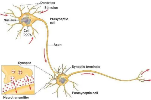
connected to another neuron’s dendrites. When a neuron fires, the electrical signal is propagated along its axon, and when it reaches the axon’s terminals, neurotransmitters are released into the synapse and to the dendrites of the next neuron (Figure 1.16).

These neurotransmitters can have an excitatory or an inhibitory effect. If they have an excitatory effect, they will alter the chemical properties of the receptor’s membrane, causing an ionic flow through the cell membrane and increasing the receiving neuron’s electric potential, leading to the generation of an action potential - an electric signal that propagates along the neuron, from the dendrites through the soma and the axon and into the next neuron. On the other hand, if the neurotransmitters have an inhibitory effect, they will cause a modification of the chemical properties of the receptor’s membrane, leading to an ionic flow and a reduction of the receiving neuron’s electrical potential, putting it in a state less likely to generate an action potential. However, in a more realistic model of the brain, each neuron receives inputs and sends outputs from and to hundreds of thousands of other neurons. All the excitatory and inhibitory inputs a neuron receives at a given time are averaged inside the soma and may or may not generate a new action potential. Information processing in neural networks is dependent not only on this intracellular averaging of the electric potential, but also on the firing frequency and fluctuations of firing frequency with time.

Figure 1.16 – Neuron’s structure and stimulus propagation diagram. Adapted from

(46)

21

1.3.2. EEG RECORDING

When a neuron generates an action potential an electromagnetic field is generated, with the neuron acting as an electric dipole (Figure 1.17a). However, the action potentials are too transient to sum up to a measurable signal recorded from the scalp. Instead, it is believed that the EEG signal results from the aggregate of electromagnetic fields produced by excitatory and inhibitory postsynaptic potentials (Kutz, 2003). Additionally, only electric fields orthogonal to the electrode surface can be measured by the EEG electrodes. For this reason, only postsynaptic potentials generated by neurons that are perpendicular to the scalp surface can contribute to the EEG signal.

The EEG output will be a series of waveforms, or channels, each representing the electrical activity of the brain for a different location on the scalp. In a classical referential montage, each channel’s waveform is obtained by subtracting the signal of a referential electrode from the signal of a scalp electrode (Figure 1.17b).

To guide the placement of the electrodes on the scalp, the International 10-20 system is usually used. This system is a globally recognized method for EEG scalp electrode location, where each electrode is named with a letter and a number. The letter (F, C, T, P or O) indicates the location on the scalp in terms of cortical region (Frontal, Central, Temporal, Parietal or Occipital, respectively) and the number defines hemisphere location – even numbers for

Figure 1.17 – Action potential being generated and propagated along the axon of a neuron (a) and a diagram illustrating a

(47)

22

electrodes on the right hemisphere, odd numbers for left hemisphere locations. Electrodes on the midline are named with a ‘z’ instead of a number (e.g. ‘Pz’ for the midline electrode on the parietal region of the cortex) (Figure 1.18).

LIMITATIONS

Although EEG provides a method of measuring electrical activity in the brain with high temporal resolution, one of its major limitations is its poor spatial resolution. The electromagnetic fields generated by groups of neurons are influenced by differences in conductivity between the cortical surface, cerebrospinal fluid and skull, making source localization a difficult task – a given electrode will pick up not only the electrical signal from a set of neurons in the cortex directly underneath it, but also the signal from sets of neurons that are located further away from that electrode. Finding the underlying cortical sources of

Figure 1.18 – Placement of electrodes on the scalp according to the International 10-20 system.

(48)

23

activity through signals measured on the scalp is known as the inverse problem. Solutions for this problem usually assume a model of the source (the dipole model being the most common) and a model of the head. These models can be described in various ways, which means that there is usually more than one possible solution to the inverse problem. Anatomical and functional constraints, highly variable between individuals, are an additional difficulty to accurate head and source modeling, and consequently to solving the inverse problem (Cuffin, 1998, Michel et al., 2004).

Additional limitations of this method include the fact that EEG can only record signals originating in the cortical surface (and is therefore insensitive to deeper structures of the brain) and also its vulnerability to movement artifacts. The electrical signals generated by the neurons and captured by the scalp electrodes are very small in amplitude, and recording is often contaminated by muscle movements that generate electrical signals of higher amplitude, such as those originating from head or eye movement (such as blinks).

TYPICAL ACTIVITY

The electrical activity in an EEG measurement is usually characterized by rhythmic and transient activity. The rhythmic activity can be separated into five frequency bands:

• Delta band (< 4 Hz): this frequency is characteristic of EEG recordings of babies or of

sleeping adults;

• Theta band (4 to 8 Hz): this frequency is often observed in EEG recordings of young

children or in adults in a state of drowsiness or arousal;

• Alpha (8 to 12 Hz): this frequency is observed in the EEG recordings of adults in an

awake, relaxed but not drowsy state, with eyes closed;

• Beta (13 to 30 Hz): this frequency is characteristic of alert or active concentration

states;

• Gamma (> 30 Hz): this frequency is present in EEG recordings taken during

performance of complex sensory processing and working memory tasks; high frequency oscillations (> 100Hz) however, may be indicative of epilepsy (Zijlmans et al., 2011).

The presence of transient activity such as spikes and spindles is considered common in recordings of sleep states. However, if detected in recordings of awake subjects it can be an indicator of seizure activity.

Analysis of the anatomical and functional basis of autism spectrum conditions using magnetic resonance imaging and electroencephalography

UNIVERSIDADE DE LISBOA

Analysis of the Anatomical and F

basis of Autism Spectrum C

Magnetic Resonance Imaging and

Electroencephalography

Ana Maria Ferreira Paradela Catarino

UNIVERSIDADE DE LISBOA

F

ACULDADE DE

C

IÊNCIAS

Analysis of the Anatomical and Functional

Autism Spectrum Conditions

Magnetic Resonance Imaging and

lectroencephalography

Ana Maria Ferreira Paradela Catarino

unctional

onditions using

Magnetic Resonance Imaging and

UNIVERSIDADE DE LISBOA

Analysis of the Anatomical and Functional

basis of Autism Spectrum Conditions

Magnetic Resonance Imaging and

Electroencephalography

Ana Maria Ferreira Paradela Catarino

UNIVERSIDADE DE LISBOA

F

ACULDADE DE

C

IÊNCIAS

Analysis of the Anatomical and Functional

basis of Autism Spectrum Conditions

Magnetic Resonance Imaging and

Electroencephalography

Ana Maria Ferreira Paradela Catarino

Analysis of the Anatomical and Functional

basis of Autism Spectrum Conditions using

CONTENTS

LIST OF FIGURES

LIST OF TABLES

LIST OF ABBREVIATIONS

ABSTRACT

RESUMO

P

UBLICATIONS

ACKNOWLEDGEMENTS

1.

G

ENERAL

I

NTRODUCTION

1.1.

A

S

C

1.2.

M

R

I

1.3.

E