❊♥s❛✐♦s ❊❝♦♥ô♠✐❝♦s
❊s❝♦❧❛ ❞❡
Pós✲●r❛❞✉❛çã♦
❡♠ ❊❝♦♥♦♠✐❛
❞❛ ❋✉♥❞❛çã♦
●❡t✉❧✐♦ ❱❛r❣❛s
◆◦ ✸✺✷ ■❙❙◆ ✵✶✵✹✲✽✾✶✵
❚❤❡ ■♠♣♦rt❛♥❝❡ ♦❢ ❈♦♠♠♦♥✲❈②❝❧✐❝❛❧ ❋❡❛✲
t✉r❡s ✐♥ ❱❆❘ ❆♥❛❧②s✐s✿ ❆ ▼♦♥t❡✲❈❛r❧♦ ❙t✉❞②
✭Pr❡❧✐♠✐♥❛r② ❱❡rs✐♦♥✮
❋❛rs❤✐❞ ❱❛❤✐❞✱ ❏♦ã♦ ❱✐❝t♦r ■ss❧❡r
❖s ❛rt✐❣♦s ♣✉❜❧✐❝❛❞♦s sã♦ ❞❡ ✐♥t❡✐r❛ r❡s♣♦♥s❛❜✐❧✐❞❛❞❡ ❞❡ s❡✉s ❛✉t♦r❡s✳ ❆s
♦♣✐♥✐õ❡s ♥❡❧❡s ❡♠✐t✐❞❛s ♥ã♦ ❡①♣r✐♠❡♠✱ ♥❡❝❡ss❛r✐❛♠❡♥t❡✱ ♦ ♣♦♥t♦ ❞❡ ✈✐st❛ ❞❛
❋✉♥❞❛çã♦ ●❡t✉❧✐♦ ❱❛r❣❛s✳
❊❙❈❖▲❆ ❉❊ PÓ❙✲●❘❆❉❯❆➬➹❖ ❊▼ ❊❈❖◆❖▼■❆ ❉✐r❡t♦r ●❡r❛❧✿ ❘❡♥❛t♦ ❋r❛❣❡❧❧✐ ❈❛r❞♦s♦
❉✐r❡t♦r ❞❡ ❊♥s✐♥♦✿ ▲✉✐s ❍❡♥r✐q✉❡ ❇❡rt♦❧✐♥♦ ❇r❛✐❞♦ ❉✐r❡t♦r ❞❡ P❡sq✉✐s❛✿ ❏♦ã♦ ❱✐❝t♦r ■ss❧❡r
❉✐r❡t♦r ❞❡ P✉❜❧✐❝❛çõ❡s ❈✐❡♥tí✜❝❛s✿ ❘✐❝❛r❞♦ ❞❡ ❖❧✐✈❡✐r❛ ❈❛✈❛❧❝❛♥t✐
❱❛❤✐❞✱ ❋❛rs❤✐❞
❚❤❡ ■♠♣♦rt❛♥❝❡ ♦❢ ❈♦♠♠♦♥✲❈②❝❧✐❝❛❧ ❋❡❛t✉r❡s ✐♥ ❱❆❘ ❆♥❛❧②s✐s✿ ❆ ▼♦♥t❡✲❈❛r❧♦ ❙t✉❞② ✭Pr❡❧✐♠✐♥❛r② ❱❡rs✐♦♥✮✴
❋❛rs❤✐❞ ❱❛❤✐❞✱ ❏♦ã♦ ❱✐❝t♦r ■ss❧❡r ✕ ❘✐♦ ❞❡ ❏❛♥❡✐r♦ ✿ ❋●❱✱❊P●❊✱ ✷✵✶✵
✭❊♥s❛✐♦s ❊❝♦♥ô♠✐❝♦s❀ ✸✺✷✮ ■♥❝❧✉✐ ❜✐❜❧✐♦❣r❛❢✐❛✳
The Importance of Common-Cyclical Features in VAR
Analysis: A Monte-Carlo Study
¤
Farshid Vahid
Depart ment of Economet rics and Business St at istics
Monash University
Clayt on, Vict oria 3168
Aust ralia
[email protected]
João Vict or Issler
Graduat e School of Economics – EPGE
Get ulio Vargas Foundat ion
Praia de Bot afogo 190 s. 1125-8
Rio de Janeiro, RJ 22253-900
Brazil
[email protected]
August 1999, preliminary version, comments are welcome.
¤T his paper was writ t en while João Vict or Issler was visit ing Monash University, which hospit alty is
A bst r act
Despite the belief, support ed by recent applied research, that aggregate data dis-play short -run comovement, t here has been lit tle discussion about t he econometric consequences of t hese dat a “ feat ures.” We use exhaustive Mont e-Carlo simulations t o investigat e t he importance of restrict ions implied by common-cyclical feat ures for est imat es and forecast s based on vect or aut oregressive and error correct ion models. First , we show t hat the “ best ” empirical model developed wit hout common cycles re-st rict ions need not nere-st t he “ bere-st ” model developed wit h those rere-st rict ions, due t o t he use of information criteria for choosing the lag order of t he two alternat ive models. Second, we show t hat t he costs of ignoring common-cyclical feat ures in VAR analysis may be high in t erms of forecast ing accuracy and e¢ ciency of est imat es of variance decomposit ion coe¢ cients. Alt hough t hese costs are more pronounced when t he lag order of VAR models are known, t hey are also non-t rivial when it is selected using t he conventional t ools available to applied researchers. T hird, we …nd t hat if the dat a have common-cyclical feat ures and t he researcher want s to use an informat ion crit erium to select the lag length, t he Hannan-Quinn crit erium is t he most appropriat e, since t he Akaike and the Schwarz criteria have a t endency t o over- and under-predict t he lag length respectively in our simulat ions.
1. I nt r oduct ion
Common-cyclical movement s in det rended economic variables have been so prevalent t hat
t hey have acquired t he st at us of “ stylized fact s.” Lucas(1977) stat es t hat t he main regularit ies
observed in cyclical ‡uct uat ions of economic t ime series are in t heir comovement, which he
itemizes as follows:
(i) Out put movement s across broadly de…ned sect ors move t oget her. (In Mit chell’s
t erminology, t hey exhibit high conformity; in modern t ime series language, t hey
have high coherence.) (ii) Product ion of producer and consumer durables exhibit
much great er amplit ude t han does t he product ion of nondurables. (iii)
Produc-t ion and prices of agriculProduc-t ural goods and naProduc-t ural resources have lower Produc-than
av-erage conformity. (iv) Business pro…ts show high conformity and much higher
amplit ude t han other series. (v) Prices generally are procyclical. (vi) Short
-t erm in-t eres-t ra-t es are procyclical; long--t erm ra-t es sligh-t ly so. (vii) Mone-t ary
aggregat es and velocity measures are procyclical.
From an empirical st andpoint common cycles have been shown t o be a “ feat ure” of a
va-riety of macroeconomic dat a set s. For example, Campbell and Mankiw(1989) …nd a common
cycle between consumpt ion and income for most G-7 count ries. Engle and Kozicki(1993) …nd
common int ernat ional cycles using GNP dat a for OECD count ries. For US dat a, Issler and
Vahid(1998) …nd common cycles for macroeconomic aggregat es and Engle and Issler(1995)
and Carlino and Sill(1998) …nd common cycles for sect oral and regional GNPs respect ively.
Similar t o most applied macroeconomic research done in t he last …ft een years, t hese st
ud-ies invest igat ed common-cyclical feat ures using vect or-aut oregressive (VAR) or vector
error-correct ion (VEC) models.
Alt hough VAR and VEC models have become t he “ working horse” of macroeconomet ric
st udies, one of t heir short comings is t he excessive number of paramet ers relative t o t he
average sample size one is usually forced t o work wit h. For example, when dealing wit h
post -war quart erly dat a, and a VAR wit h t hree variables and eight lags, t here are seventy
…ve mean parameters t o be est imat ed from about two hundred dat a point s on each variable.
Coint egrat ion places some rest rict ions on VAR coe¢ cient s, especially when coint egrat ing
vect ors are brought in from economic t heory; see Engle and Granger(1987). In t hese cases,
t he reduct ion in t he number of free coe¢ cient s is not overwhelming. If t he t hree-variable
syst em has one known coint egrat ing vect or, t he number of free paramet ers reduces from
reduce t he number of condit ional-mean paramet ers est imat ed in VEC models by considering
t he rest rict ions implied by t hem; see Vahid and Engle(1993). If t he t hree variables in t he
VEC model share one common cycle, t hen t he number of mean paramet ers reduces from
sixty nine t o twenty seven.
The object ive of this paper is t o invest igat e t he import ance of rest rict ions implied by
common-cyclical feat ures for forecast s, impulse-response funct ions, and variance-decomposit ion
of forecast errors of economic t ime-series based on VAR and VEC models. As far as we know,
no work has st udied t he e¤ect s of t hese rest rict ions. However, considerable e¤ort has been
put in examining t he import ance of long-run comovement const raint s in VAR models,
espe-cially for forecast ing; see, among ot hers, Engle and Yoo(1987), Clement s and Hendry(1995),
and Lin and Tsay(1996).
As shown by Engle and Yoo, t he forecast ing gains of imposing long-run const raint s
hap-pens as t he horizon get s large. In fact , in t heir simulat ions, t he unconst rained VAR forecast s
bet t er t han t he VEC model for short horizons. Because for long horizons forecast ing
uncer-t ainuncer-ty geuncer-t s helplessly large uncer-t ime-series models are mosuncer-t useful for forecasuncer-t ing in shoruncer-t horizons.
Hence, t he payo¤ of investigat ing t hese short -run const raint s are big relat ive t o t hose of
in-vest igating long-run const raint s, since t hey may be a way of improving t he e¤ect iveness of
t ime-series models for horizons where t hey are most useful.
We assess t he e¤ect s of common-cyclical feat ures on VAR and VEC models using Mont
e-Carlo simulat ions. The focus here is on t he small-sample propert ies of t he est imat es of
impulseresponse funct ions and variancedecomposit ion of forecast errors, as well as on out
-of-sample forecast ing accuracy measures. We design t he simulat ions in such a way t hat t he
result s would be relevant for applied macroeconomist s dealing wit h a limit ed number of dat a
point s and t rying t o est imate a relat ively large number of paramet ers. To t hat end, we
consider a variety of Dat a Generat ing Processes (DGPs) and sample sizes, which are kept
close t o t he “ typical” dat a applied researchers oft en encount er in pract ice.
VAR and VEC models wit h common cycles fall int o t he general cat egory of
t heir paramet er mat rices1. Researchers may be reluct ant t o incorporat e t hese paramet er
rest rict ions for a purely st at ist ical reason relat ed t o t he asymmet ry of t he consequences of
over- versus under-paramet rizat ion of economet ric models. One might t hink t hat failing t o
incorporat e common-cycle rest rict ions when t hey are t rue will only cause ine¢ ciency, while
imposing t hem when t hey are false will cause inconsist ency. Hence, it may seem wiser t o live
wit h a possibly ine¢ cient unconst rained model rat her t han a misspeci…ed inconsist ent model.
The fact t hat all models are most probably misspeci…ed, and t he large body of empirical
evidence on t he superior forecast performance of parsimonious models notwit hst anding, t his
reasoning would be correct only if t he empirical model t hat does not have common cycles
built int o it nest s t he empirical model wit h common cycles. However, we show t hat , using
t he average t ools of an applied researcher, and t he same dat a set , t he “ best ” empirical model
developed wit hout common-cycle rest rict ions need not nest t he “ best ” model developed wit h
t hose rest rict ions.
The underlying reason for t his rat her paradoxical result has t o do wit h t he select ion of lag
order for t he two alt ernat ive models. The common pract ice in VAR analysis is t o use a
model-select ion crit erium t o choose t he lag lengt h. St andard model-model-select ion crit eria may …nd t oo
small a lag lengt h of reduced-rank VARs simply because t his is t he only possible way available
t o achieve parsimony. However, if t he lag lengt h and t he VAR rank are chosen simult aneously,
as suggest ed by Lüt kepohl(1993, page 202), the lag lengt h select ed for reduced-rank VARs
can be pot entially bigger t han t hat select ed by t he st andard crit erium. For example, t he
Schwarz crit erium might choose a VAR(1) as t he best unconst rained VAR, while t he same
crit erium might choose a VAR(4) with one common cycle for t he same dat a set . Obviously, a
VAR(1) cannot nest a VAR(4) wit h common cycles. Hence, t he considerat ion of comovement
in t he model select ion st age may drast ically alt er t he …nal model chosen.
Our simulat ions reveal t hat , when the t rue DGP is a reduced-rank VAR or VEC model,
t he lag lengt h chosen by t he st andard model-select ion crit eria and t hat chosen when rank
1Classic references on reduced-rank VAR’s include Velu, Reinsel and Wickern(1986), Ahn and
and order are select ed simult aneously can be quit e di¤erent . St andard informat ion crit eria
which place a st rong penalty on overparamet erizat ion, such as t he Schwarz or Hannan-Quinn
crit eria, may choose too small a lag-lengt h when t he t rue model has common cycles. However,
t hey can improve considerably if t he rank order is select ed simult aneously wit h t he lag lengt h.
We …nd st rong evidence in favor of t he ability of t he Hannan-Quinn crit erium in choosing t he
correct lag and rank order overall. Regarding t he Akaike informat ion crit erium, we observe
t hat it s t endency t o choose an overparamet erized model when t he lag order and rank are
select ed simult aneously worsens compared t o t he case when only t he lag lengt h is select ed.
For horizons up t o sixt een periods ahead, using several measures of forecast ing accuracy,
we …nd t hat forecast s produced by t he “ best ” reduced-rank model are generally superior t o
t hose produced by t he “ best ” model when only lag-order is select ed. The same conclusions
are obt ained when comparing t he variance decomposit ions of t he “ best ” reduced rank model
wit h t hat of t he “ best ” full rank model when t he sample size is 2002. Indeed, on average, if
t he Hannan-Quinn crit erium is used t o select lag order and rank, forecast ing accuracy can be
improved by up t o 20%, and mean-squared-error of predict ing t he t rue variance cont ribut ion
can be cut up t o half in short horizons. This is a sizable e¤ect which illust rat es t he pot ent ial
gains associat ed t o considering common-cyclical feat ures whenever t hey exist .
The out line of t he paper is as follows. Section 2 st at es t he reduced-rank rest rict ions t hat
common-cyclical ‡uct uat ions impose on paramet ers of VAR and VEC models, and discusses
t he relat ive merit s of det ermining t he rank order by st at ist ical t est s versus informat ion
cri-t eria. Seccri-t ion 3 explains cri-t he design of cri-t he Moncri-t e-Carlo design used cri-t hroughoucri-t cri-t he paper.
Sect ion 4 present s t he simulat ion results for a small syst em of t hree variables and sect ion 5
present s t he same result s for a larger syst em of six variables. Finally, sect ion 6 summarizes
t he main conclusions of t he paper.
2Not ice t hat in t he t ext book example Lüt kepohl(1993, pp. 202-3) lag select ion was ident ical whet her or
2. Com m on cy cles in VA R and V EC m odels
To mat ch t he stylized fact s of most macroeconomic variables, we assume t hat t he object ive
of research is t o build a t ime series model for t he growt h rat e of a vect or of n economic
variables. We denote t he level of t hese variables at t imet by Yt, t heir logarit hms by yt, and
t heir growt h rat es (i.e. t he …rst di¤erence of t he logarit hm of Yt) by ¢yt. We make t he
reasonable assumpt ion t hat ¢yt is st at ionary, add t he assumpt ion t hat ¢yt has mean zero t o
simplify not at ion, wit hout loss of generality, and st art wit h t he Wold represent at ion of ¢yt:
¢yt = C (L ) "t; (2.1)
whereC (L ) = P 1
j = 0CjLj is a mat rix polynomial in t he lag operat or L, Lkzt = zt ¡ k, wit h
C0 = In. From t he work of Beveridge and Nelson(1981) and St ock and Wat son(1988) it is
possible t o decompose t he log-level seriesyt int o common t rends and cycles (which we refer
t o as t he Beveridge-Nelson-St ock-Wat son — or BNSW for short — decomposit ion). Using
t he ident ity C (L ) = C (1) + ¢ C¤(L ), disconsidering t he init ial values iny
0, and int egrat ing
bot h sides of (2.1) we get3:
yt = C (1)
t
X
j = 1
"j + C¤(L ) "t
= Tt + Ct; (2.2)
whereTt = C (1)
Pt
j = 1"j and Ct = C¤(L ) "t st ack respect ively t he t rend and cyclical
com-ponent s of yt. In the BNSW decomposit ion t he n variables in yt are decomposed int o n
random-walk component s (st ochast ic t rends) and n stat ionary component s (st ochast ic
cy-cles). If C (1) has rank n¡ q (q > 0), t he st ochast ic t rends in yt can be charact erized as
linear combinat ions of only n¡ qcommon random walks, in which caseyt is said t o be
coin-t egracoin-t ed or have common scoin-t ochascoin-t ic coin-t rends, wicoin-t hqlinearly independent coint egrating vect ors
st acked in t he mat rix®0; see Engle and Granger(1987). IfC¤(L )has rankr (n¡ r > 0), t hen
t he st ochast ic cycles inyt can be charact erized as linear combinat ions ofr common st ochast ic
cycles, wit hn¡ r cofeat ure vect ors st acked in t he mat rix ®e0; see Vahid and Engle(1993). In
t his paper, we invest igat e t he cost s of ignoring t his singularity in t he st ochast ic cyclesCt.
If there aren¡ q common t rends in t he syst em, t hen a vect or error-correct ion (VEC)
model,
¢yt = A1¢yt ¡ 1+ ::: + Ap¢yt ¡ p+ ° ®0yt ¡ 1+ "t
=
·
A1 : : : Ap ° ®0
¸ 2 6 6 6 6 6 6 6 6 4
¢ yt ¡ 1
.. .
¢ yt ¡ p
yt ¡ 1
3 7 7 7 7 7 7 7 7 5
+ "t; (2.3)
would be a parsimonious represent at ion for yt relat ive t o t he VAR in log-levels, where t he
columns of t hen£qmat rix®are t he coint egrat ing vect ors and° is the adjust ment -coe¢ cient
mat rix. If t here is no coint egrat ion, t hen t he t erm ° ®0y
t ¡ 1 on the right -hand side of (2.3)
vanishes and t he model reduces t o a VAR in …rst di¤erences. Hence, in what follows, wit hout
loss of generality, we focus our at t ent ion on t he VEC model.
If t here are r common stochast ic cycles in yt, t he mat rix
·
A1 : : : Ap ° ®0
¸
, which
includes all t he paramet ers in t he condit ional mean of ¢yt, must have rank r. This is a
consequence of t he fact t hat C¤(L ) in (2.2) has rank r, which implies t hat t here are exact ly
n¡ r non-colinear linear combinat ions of yt which are random walks and do not exhibit any
cycles. Since t he …rst di¤erences of t hesen ¡ r linear combinat ions are whit e noise, t hey
are unpredict able using t he past . Hence,
·
A1 : : : Ap ° ®0
¸
must have rank r, wit h a
common null-space. This implies t hat t he VEC model has it self t he following parsimonious
represent at ion:
2 6 4 In¡ r
e
®¤0
0 Ir
3 7
5¢ yt =
2 6
4 0 ¢¢¢ 0 0
A¤
1 ¢¢¢ A¤p (° ®0) ¤ 3 7 5 2 6 6 6 6 6 6 6 6 4
¢ yt ¡ 1
.. .
¢ yt ¡ p
yt ¡ 1
3 7 7 7 7 7 7 7 7 5
where t he cofeat ure mat rix ®e0=
·
In ¡ r ®e¤0
¸
, which st acks t he linearly-independent
combi-nat ions of ¢ yt t hat eliminat es t he common serial correlat ion in t he syst em’s component s, is
rot at ed in order t o yield ann¡ r ident ity sub-mat rix in it s …rst n¡ r rows and columns,A¤ i
and(° ®0)¤
represent respect ively t he part it ions ofAi and° ®0corresponding to t he remaining
r equat ions in t he syst em, and vt =
2 6
4 In ¡ r ®~
¤0
0 Ir
3 7
5 "t. Since
2 6
4 In¡ r ®~
¤0
0 Ir
3 7
5 is invert ible, it is
possible t o recover (2.3) from (2.4).
Common-cycle const raint s imply import ant rest rict ions for t he impulse-response
func-t ions, variance-decomposifunc-t ion of forecasfunc-t errors, and mulfunc-t i-sfunc-t ep ahead forecasfunc-t s. The
exis-t ence of r common cycles implies t hat t here aren¡ r non-collinear linear combinat ions of
¢yt which are whit e noise. Thus, from (2.1), all mat ricesCi, i = 1; 2;¢¢¢, must have rank r.
These mat ricesCi, usually normalized t o be consist ent wit h ort hogonal errors, form t he basis
of impulse-response funct ions and t he component s of forecast -error variance decomposit ions.
For example, when t hey are post -mult iplied by t he cholesky fact or of t he variance-covariance
mat rix of "t, t hey yield t he so-called ort hogonalized impulse responses. Hence, it becomes
clear t hat common cycles imply t hat t he impulse responses of di¤erent variables t o t he same
shocks are linearly dependent . T herefore, if t he object s of int erest are t he impulse responses
(or variance decomposit ions of forecast errors) of¢yt, common-cycle rest rict ions can be used
t o achieve parsimony and t heir e¢ cient est imat ion in t his mult ivariat e cont ext .
A similar argument applies t o forecast s of ¢yt at horizon h. These can be recursively
calculat ed from:
¢yft+ h = A1¢yt+ h¡ 1f + ::: + Ap¢yft + h¡ p+ ¦ y f
t + h¡ 1 (2.5)
where t he superscript f st ands for forecast s using informat ion up t o period t, ¦ = ° ®0,
and act ual variables are used inst ead of forecast s on t he right -hand side where available.
Since common cycles imply t hat t he mat rix
·
A1 : : : Ap ¦
¸
has reduced rank, equat ion
(2.5) clearly shows t hat t hey will also imply t hat t he forecast s of ¢yt at any horizon will be
linearly dependent . Again, if forecast ing is t he object ive of t he mult ivariat e model building
est imat ion.
In a VAR context above, t here are two ways in which parsimony can be achieved. The
…rst is by imposing long-run const raint s (coint egrat ion), i.e., equat ion (2.3), and t he second
is by imposing short -run const raint s (common cycles), i.e., equat ion (2.4). T he lit erat ure
on forecast ing has focused on long-run const raint s; see, for example, Engle and Yoo(1987),
Clement s and Hendry(1995), and Lin and Tsay(1996). As argued in t he Int roduct ion, t he
payo¤ of invest igat ing short-run const raint s are large relat ive to t hose of investigat ing
long-run const raint s, which mot ivat es our present research e¤ort .
2.1. I nfor mat ion cr it er i a for r educed-r ank m odel s
Our mot ivat ion is t o build VAR-based models for ¢yt which can be used for forecast ing,
impulse-response or variance-decomposit ion analysis. A crit ical st ep in const ruct ing t hese
models is how t o select t he lag lengt h of t he VAR (VEC). Model-select ion crit eria are oft en
used in pract ice t o select lag lengt h. In principle, they are useful because t hey do not favor
any speci…c model against ot hers (null versus alt ernat ive in hypot hesis t est ing, for example);
see t he discussion in Granger, King and Whit e(1995). Such crit eria may choose di¤erent
lag orders depending on whet her or not we allow for reduced-rank paramet er mat rices in
t he VEC model4. Given t he pot ent ial e¢ ciency gains of using common-cycle rest rict ions,
we invest igat e empirically t he performance of widely-used selection crit eria when only lag
lengt h is select ed and when lag lengt h and rank order are select ed. Final result s can t hen be
compared t o help building a st rat egy for empirical work.
Following Lüt kepohl(1993), we focus on the Akaike, Hannan-Quinn and Schwarz
infor-mat ion crit eria for t he simult aneous select ion of lag and rank orders in VARs (VEC models).
For t he VEC model in equat ion (2.3), we assume t hat coint egrat ing vectors are eit her known
4Vahid and Engle(1993) focused on t est ing t heories t hat implied common cycles wit hin a VEC-model
from t heory, or are correct ly est imat ed in advance. This is done here for simplicity, avoiding
t he well known problem of dealing simult aneously wit h int egrat ed and st at ionary regressors
in VEC models; see Toda and Phillips(1993), for example. Under this assumpt ion, t he VEC
model in (2.3) can be writ t en as:
¢yt =
·
A1 : : : Ap °
¸ 2 6 6 6 6 6 6 6 6 4
¢ yt¡ 1
.. .
¢ yt¡ p
®0y t¡ 1 3 7 7 7 7 7 7 7 7 5
+ "t: (2.6)
The lag order pand t he number of common cyclesr, which is t he rank of
·
A1 : : : Ap °
¸
,
can be simult aneously chosen t o minimize one of t he following model select ion crit eria5:
AI C(p; r ) = ln
¯ ¯
¯§^" (p; r )
¯ ¯ ¯+ 2
T £ r £ (np + n¡ r + q) (2.7)
H Q (p; r ) = ln
¯ ¯
¯§^" (p; r )
¯ ¯
¯+ 2 ln lnT
T £ r £ (np + n¡ r + q) (2.8)
SC (p; r ) = ln
¯ ¯
¯§^" (p; r )
¯ ¯
¯+ lnT
T £ r £ (np + n¡ r + q) (2.9)
whereqis t he number of coint egrat ing vect ors,n is t he dimension of t he system,r is t he rank
of VEC model, pis t he number of lagged di¤erences in t he model, §^"(p; r ) is the est imat ed
variance-covariance mat rix of t he errors of t he VEC model wit hplags and rank r; andT is
t he number of observat ions. Vahid and Engle(1993) showed t hat r ¸ q; which implies t hat ,
given q, models of rank smaller t han qneed not be considered.
Calculat ing the informat ion crit eria in (2.7)-(2.9) for full-rank models(r = n) is st raight
-forward, since t hey can be est imat ed, equat ion by equat ion, using OLS. On t he ot her hand,
for reduced-rank models, comput ing t hese crit eria for di¤erent p and r may seem di¢ cult ,
since one may t hink t hat t heir est imat ion is required. However, t he following Lemma st at es
a well known result t hat relat esln
¯ ¯
¯§^"(p; r )
¯ ¯
¯ t o t he squared canonical correlat ions between
5When t he variables are not coint egrat ed q = 0, and t hese crit eria are t he same as t hose suggest ed in
¢yt and
·
¢y0
t ¡ 1 ¢¢¢ ¢y0t¡ p (®0yt ¡ 1)0
¸0
making comput at ion of t hese crit eria in t his case
also st raight forward.
L em m a 2.1. The minimum ofln¯¯¯T1P Tt = 1"t"0t
¯ ¯
¯under t he assumpt ion t hat ·
A1 : : : Ap °
¸
has rankr is
ln ¯ ¯ ¯ ¯ ¯ 1 T T X
t = 1
¢yt¢y0t
¯ ¯ ¯ ¯ ¯+ n X
i = n¡ r + 1
ln (1¡ ¸i);
where¸1 < ¸2 < ¢¢¢< ¸n are t he sample squared canonical correlat ions between¢yt and
t he set of regressorsx0 t ´
·
¢y0
t ¡ 1 ¢¢¢ ¢yt ¡ p0 (®0yt¡ 1)0
¸
: T he sample squared canonical
correlat ions are t he eigenvalues of
0 @
T
X
t= p+ 1
¢yt¢yt0
1 A
¡ 10
@
T
X
t = p+ 1
¢ytx0t
1 A 0 @ T X
t= p+ 1
xtx0t
1 A
¡ 10
@
T
X
t = p+ 1
xt¢yt0
1 A :
Pr oof. See Tso(1981).
This lemma shows t hat , aft er dropping t he common const ant t ermln
¯ ¯
¯T1P Tt= 1¢yt¢yt0
¯ ¯ ¯in (2.7)-(2.9), t hese model-select ion crit eria can be expressed in t erms of t he eigenvalues(¸i)
as:
AI C(p; r ) =
n
X
i = n ¡ r + 1
ln (1¡ ¸i (p)) +
2
T £ r £ (np + n¡ r + q) (2.10)
H Q (p; r ) =
n
X
i = n ¡ r + 1
ln (1¡ ¸i (p)) +
2 ln lnT
T £ r £ (np + n¡ r + q) (2.11)
SC (p; r ) =
n
X
i = n ¡ r + 1
ln (1¡ ¸i (p)) +
lnT
T £ r £ (np + n¡ r + q) : (2.12)
Hence, for …xed p; t he model-select ion crit eria for any rank can be easily calculat ed aft er
t hese eigenvalues are comput ed. The eigenvalues can be easily calculat ed by any st at ist ical
program which has a canonical correlat ion procedure6. Not ice t hat , for …xedT,n andq, t he
model-select ion crit eria in (2.10)-(2.12) depend only on t he lag lengt hpand on t he rank of t he
paramet er mat rices in t he VEC model r, i.e., VEC models where t he number of coint egrat ing
vect ors is known.
6For example, SAS or STATA, or any mat rix program such as GAUSS, or by slight ly modifying any of t he
3. M ont e-Car lo design
If samples are “ large” and t he variables have common cycles, our int uit ion t ells us t hat
ignoring t hem will not be very harmful. T his is based on t he expect at ion t hat wit h “ large”
samples, lag-order select ion is likely t o be unambiguous, and paramet er est imat es will be
precise, so t hat t he reduced rank const raint s will be (approximat ely) t rue for t he est imat ed
paramet ers, even when t hey are not imposed at t he est imat ion st age. Hence, t he est imat ed
models wit h or wit hout common-cycle rest rict ions will be so close, t hat t heir result s for
forecast ing, impulse-response, and variance-decomposit ion analysis will be very similar.
This int uit ion should not , however, be carried over t o the case of “ small” samples. As a
mat t er of fact , e¢ ciency gains are pot ent ially relevant when sample sizes are small and
de-grees of freedom are scarce. In t his cont ext , using informat ion crit eria t o select lag order may
not be unambiguous. The st andard pract ice is t o disregard t he possibility of reduced-rank
models in t he formula of widely-used model-select ion crit eria, i.e., set r = n in (2.10)-(2.12).
This creat es t he pot ent ial problem of model misspeci…cat ion in select ing lag lengt h. Indeed,
select ing lag order imposing t hat t he model is full-rank can yield a complet ely di¤erent result
t han select ing lag order and rank simult aneously. We invest igat e t his issue using 1000
simu-lat ions of 100 reduced-rank VARs wit h eit her 100 or 200 observations each, t abusimu-lat ing result s
when lag lengt h alone is chosen and when rank and lag lengt h are chosen simult aneously.
To make present at ion manageable, we chose t o work wit h t hree- and six-dimensional
VARs. In t he applied macroeconomics lit erat ure, models t hat only consider t he real side of
t he economy are usually t hree-dimensional. For example, in t est ing t he real-business-cycle
model in King, Plosser and Rebelo(1998), King et al.(1991) est imat e a VAR including out put ,
consumpt ion, and invest ment . Issler and Ferreira(1998) use a VAR including out put , labor,
and capit al input s, t o est imat e long-run elast icit ies of t he aggregat e product ion funct ion.
Six-dimensional VARs usually include a t ri-variat e real-variable sub-syst em, as well as a
monet ary sub-syst em, including the real money supply, real int erest rat e, and t he level of
The …rst paramet er we set in t he Mont e-Carlo design is t he lag lengt h p. It is chosen in
order t o allow eit her t he possibility of under- or over-paramet erizat ion of t he VAR (VEC)
model. This does not happen in eit her Lüt kepohl(1985) or in some simulat ions in
Nickels-burg(1982). T he …rst uses a DGP wit h a t rue lag order of 1 in his simulat ions, making
under-paramet erizat ion virt ually impossible. This favors informat ion crit eria which heavily
penalize over-paramet erizat ion, e.g., t he Schwarz crit erium7. The second set s t he t rue lag
order t o four, but t he maximum lag of four as well in t he est imat ion st age. This makes
over-paramet erizat ion impossible, favoring liberal crit eria such as t he AIC. To avoid bot h
problems, for t he t hree-dimensional syst em, we chose t he t rue lag order of 4 allowing for
models of up t o lag 8. For t he six-dimensional syst em, in order t o save degrees of freedom,
we use as t he DGP a VAR wit h two lags and allow est imat ion up t o lag six.
Next , we discuss t he choice of variance-covariance mat rix for t he VAR error "t in t he
Mont e-Carlo design. T he propert ies of est imat ed VARs are only invariant t o scaling t he
variance-covariance mat rix of t he errors by a scalar. However, t he following lemma shows
t hat in order t o cover t he ent ire space of reduced-rank VAR processes of order (p), one can …x
t he variance-covariance mat rix of "t t o be t he ident ity mat rix wit hout any loss of generality.
L em m a 3.1. Any arbit rary full rank linear t ransformat ion of a reduced-rank VAR, generat es
anot her VAR wit h t he same rank.
Pr oof. Consider aV AR(p),
yt = A1yt¡ 1+ ¢¢¢+ Apyt ¡ p+ "t:
Assume t hat P is a full rank n £ n mat rix which ort hogonalizes t he variance-covariance
mat rix of "t. De…nezt ´ Pyt, B1 ´ PA1P¡ 1 , ¢¢¢, Bp ´ PApP¡ 1, and ´t ´ P"t, where
E (´t´0t) = In. We have,
zt ´ Pyt = P A1yt ¡ 1+ ¢¢¢+ PApyt ¡ p+ P "t
7Not surprisingly, t his is exact ly t he crit erium t hat does best in choosing t he correct lag order in his
= PA1P¡ 1Pyt ¡ 1+ ¢¢¢+ PApP¡ 1Pyt ¡ p+ P"t
= B1zt ¡ 1+ ¢¢¢+ Bpzt ¡ p+ ´t: (3.1)
SinceP is of full rank, t heBi’s have t he same rank as of t heir Ai’s count erpart . Since all t he
Ai’s have t he same left null-space, so will all t heP Ai’s, and t herefore so will t heBi’s.
We now t urn t o choice of t he coe¢ cient s in t he condit ional mean of t he VAR (VEC)
model. An exhaust ive Mont e-Carlo st udy over t he ent ire model space is unfeasible. It is
cust omary, as in Lütkepohl(1985), t o choose several set s of eigenvalues for t he companion
mat rix8 of t he VAR, and t o choose arbit rary paramet er mat rices which give rise t o t hose
eigenvalues, averaging t he result s over all t hese DGPs. Alt hough t he result s generat ed from
such a design st rat egy might be useful for general t ime-series analyst s, t hey are unsuit able
for economist s who work wit h aggregat e macroeconomics dat a. This is because t he cyclical
st ruct ure (i.e. signal t o noise rat io) of models including macroeconomic aggregat es can be
quit e weak, especially for syst ems which do not cont ain a monet ary sect or. For example, t he
syst emR2(a measure similar t oR2for univariat e models which is discussed in t he Appendix)
for King et al.’s(1991) VEC model of US per-capit a income, consumpt ion, and invest ment is
0.44, whereas t he syst emR2for 160 out of t he 200 DGPs which Lüt kepohl(1985) averages over are above 0.5, and 96 of t hese are great er t han 0.8. Since t his paper is int ended primarily for
applied macroeconomist s, a design which gives too much weight t o models wit h high syst em
R2would be inappropriat e.
Here, we st art wit h a “ typical” macroeconomet ric st udy in order t o select t he DGP and
t he syst em R2 associat ed wit h it . T he data set used for choosing our paramet er values is
t he same as in King et al.(1991)9. For t he t hree-variable syst em, we considered 100 di¤erent
DGPs. Their set of paramet er values are drawn randomly from t he est imat ed asympt ot ic
95% con…dence region of t he paramet ers of reduced-rank VARs of order four. T he lat t er
8T he companion matrix of a VAR(p) is t he coe¢ cient mat rix of it s VAR(1) represent at ion. T he condit ion
for VAR(p) t o be st at ionary is t hat all of t he eigenvalues of it s companion mat rix are inside t he unit circle.
9King et al.(1991) chose a lag lengt h of eight for t heir t hree variable model and a lag lengt h of six for t heir
are based on est imat es of fourt h-order VARs of t he …rst -di¤erences of t he logarit hms of US
per-capit a privat e income, consumpt ion, and invest ment over t he period 1947.1 t o 1988.4,
in quart erly frequency. For t he six-variable model, we also considered 100 DGPs, drawned
using t he same met hod, aft er …tt ing reduced-rank VARs of order two t o t he …rst di¤erences
of logarit hms of per-capit a privat e income, consumpt ion, invest ment , real money balances,
int erest rat e and in‡at ion over t he period 1947.1 t o 1988.4. For all cases, we have been
careful t o verify t hat all of t hese randomly drawn DGPs sat isfy t he st at ionarity condit ions
for Vect or Autoregressions10.
By choosing our DGPs from t his “ plausible” subset of t he paramet er space, we believe
t hat our result s would be direct ly relevant for applied macroeconomist s. For comparison
wit h Lüt kepohl(1985), t he median of t he syst emR2measure for our generat ed t hree-variable
DGPs is between 0.5 and 0.6, wit h less t han 5% larger t han 0.7 and none great er t han 0.8.
The Mont e-Carlo simulat ion consist s of t he following:
1. Using each of t hese 100 DGPs, we generat e 1000 samples (of either 100 or 200
ob-servat ions), record t he lag lengt h chosen by t radit ional (full-rank) AIC, HQ, and SC
measures, i.e., t he informat ion crit eria st at ed in (2.10)-(2.12) whenr = n, and t he lag
lengt h and rank order chosen by t he informat ion crit eria st at ed in (2.10)-(2.12).
1. In all cases, t o reduce t he impact of init ial values on simulat ed series, we generat ed
500 observat ions. Only t he last 116 or 216 observat ions were select ed for t he
forecast ing exercise and only t he last 100 and 200 were select ed for t he
impulse-response and variance-decomposit ion exercises.
2. We t hen compare t he ability of each of t hese st rat egies of model select ion in est imat ing
t he DGP’s t rue lag lengt h and rank. This comparison allows measuring t he chance of
misspeci…cat ion arising from ignoring common-cycles at t he lag-lengt h select ion st age.
10T he range of t he absolut e value of t he maximum eigenvalue of t he t ri-variat e rank-one DGPs is
3. Based on t he informat ion-crit eria result s, a “ best ” model for each crit erium is chosen
when t radit ional (full-rank) crit eria are used and a “ best ” model for each crit erium is
also chosen when t he crit eria in (2.10)-(2.12) are used. For each type of informat ion
crit eria t hese two “ best ” models are compared regarding:
1. out -of-sample forecast ing accuracy up t o 16 periods ahead, and,
2. mean-squared-error in est imat ing variance decomposit ions of forecast errors and
impulse-response funct ions.
We t urn now t o t he speci…cs of t he exercises on forecast ing evaluat ion and on
variance-decomposit ion and impulse-response funct ion est imates.
3.1. M easur ing for ecast ing accur acy
Appropriat e evaluat ion of forecast s depends on t he speci…c use t hat the forecast s are needed
for, i.e. t he “ loss funct ion” of t he user. The fact t hat we have applied economist s as our t arget
audiencedoes not point t o any speci…c way t hat we should evaluat e t he forecast s of alt ernat ive
models. First , it is not reasonable t o impose any type of asymmet ry in evaluat ing forecast
errors. Second, a macroeconomist who models t he growt h rate of income, consumpt ion and
invest ment , might in fact be int erest ed in t he growt h rat es of income, savings and invest ment ,
or she might be int erest ed in forecast ing t he levels based on t he growt h rat es. Therefore,
it is import ant t o evaluat e t he forecast ing performance of di¤erent models on t he basis of
measures t hat are invariant t o linear t ransformat ion of forecast s at one horizon, or across
di¤erent horizons. One measure t hat sat is…es t his invariance property is t he generalized
forecast error second moment (GF E SM ) int roduced by Clements and Hendry(1994). It is
t he det erminant of t he expect ed value of t he out er product of t he vect or of st acked forecast
quart ers ahead are of int erest , t his measure will be:
GF E SM =
¯ ¯ ¯ ¯ ¯ ¯ ¯ ¯ ¯ ¯ ¯ ¯ ¯ ¯ ¯ E 0 B B B B B B B B @ ~ "t + 1
~ "t + 2
.. .
~ "t + h
1 C C C C C C C C A 0 B B B B B B B B @ ~ "t + 1
~ "t + 2
.. .
~ "t+ h
1 C C C C C C C C A
0¯¯
¯ ¯ ¯ ¯ ¯ ¯ ¯ ¯ ¯ ¯ ¯ ¯ ¯
where~"t + h is t hen-dimensional forecast error at horizonh of our n-variable model. It is
ob-vious t hat t his measure is invariant t o element ary operat ions t hat involve di¤erent variables,
and also t o element ary operat ions t hat involve t he same variable in di¤erent horizons. In
t he Mont e-Carlo, t he above expect at ion is evaluated for every model, by averaging over t he
simulat ions.
We also considered here two addit ional measures of forecast ing accuracy. T he …rst is
t he det erminant of t he mean squared forecast error mat rix at di¤erent horizons(jM SF Ehj),
and t he second is t he t race of t he mean squared forecast error mat rix (TM SF E ). The
det erminant of t heM SF E is invariant t o element ary operat ions on forecast s of di¤erent
variables at a single horizon, but it is not invariant t o element ary operat ions on forecast s
across di¤erent horizons. T he t race of t he mean squared forecast error mat rix is not invariant
t o eit her of t hese t ransformat ions.
There is one complicat ion arising from t he fact t hat we are simulat ing 100 di¤erent DGPs.
In t his case, t he simple averaging of t hese measures across di¤erent DGPs is not appropriat e,
since t he forecast errors of di¤erent DGPs do not have ident ical variance-covariance mat rices.
Lütkepohl(1985) normalizes t he forecast errors by t heir t rue variance-covariance mat rix in
each case t o get i.i.d. observat ions. Unfort unat ely, t his would be a very t ime consuming
pro-cedure for a measure likeGF E SM which involves stacked errors of many horizons. Inst ead,
we calculat e t he percent age change in t hese measures in t he “ best ” full-rank model and t he
“ best ” reduced-rank model chosen by each crit erium for every DGP, and t hen average t hese
3.2. Pr eci si on of i m pulse-r esp onse and var i ance-decomp osi t ion est i m at es
Alt hough in many cases t he object s of interest in applied st udies t hat use VAR or VEC models
are impulse-response funct ions and variance-decomposit ions of forecast errors, all simulat ion
st udies we aware of focus on forecast comparisons alone. Thus, st udying t he precision of
est imat es of impulse-response funct ions and variance-decomposit ion coe¢ cient s for di¤erent
VAR and VEC models has also a high payo¤.
Impulse-response functions and variance-decomposit ion of forecast errors di¤er from mult
i-st ep forecai-st s of VAR of VEC models in which t hey are not only non-linear funct ions of t he
est imat es of mean-paramet er mat rices but of t he variance-covariance mat rix of syst em errors
as well. Given t his added dimension t o t he problem, one cannot a priori expect t o get similar
result s t o the forecast ing exercise.
Moreover, t here a few issues t hat are speci…c t o t he analysis of impulse-response funct ions
and variance decomposit ion of forecast errors. First , errors have t o be ort hogonal for result s
t o be meaningful11. As is well known, t here are several t echniques t hat yield ort hogonal
errors. Here, we chose t o use t he Choleski decomposit ion for t he variance-covariance mat rix
t o ort hogonalize shocks, since t his is by far t he most popular met hod used in pract ice.
Second, for a t hree-variable syst em t here are nine impulse-response and variance-component
coe¢ cient s in each horizon. For a six-variable syst em t here are t hirty six. In order t o report
result s in a compact way, t he mean-squared errors of each of t hem is comput ed for t he
rank-rest rict ed and t he unrank-rest rict ed VAR model. T hen, t he percent age improvement in MSE of
t he rest rict ed model is comput ed for each of t hese coe¢ cient s. Finally, for each horizon,
t he mean percent age improvement across all coe¢ cient s is comput ed. It should be not iced
t hat t his met hod ensures t hat …nal result s do not depend on t he unit of measurement of t he
variables in the syst em. T hird, in order t o keep t he size of our t ables down t o a minimum,
only variance-decomposit ion result s are report ed, since result s for impulse responses followed
11In t his case, t he result s in our Lemma 2 are not applicable, since Mont e-Carlo result s are not independent
a very similar pat t ern t o t hose found in t he variance-decomposit ion exercise.
3.3. A benchmar k for fut ur e r efer ence
As in any simulat ion study is useful t o generat e a benchmark case t o be used for fut ure
reference. Here, we chose as a nat ural benchmark simulat ion t he case where t he researcher
knows t he t rue lag lengt h of t he VAR, t hereby ruling out any chanceof model misspeci…cat ion.
Any di¤erences between reduced-rank and full-rank VAR models re‡ect solely e¢ ciency gains
of the former.
To save space we present t he result s of t his exercise only for t he t hree-variable syst em.
Table 1 shows t he percent age improvement of di¤erent measures of forecast accuracy and of
mean-squared error (MSE) of variance-decomposit ion coe¢ cient s when reduced-rank VEC
models are allowed for. If GF E SM is considered, forecast ing accuracy can improve as much
as 73%, wit h a median improvement across all horizons and sample sizes of about 30%. If
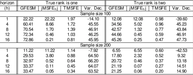
jM SF Ehj and T M SF E are considered t he gains are smaller (22% and 2% respect ively).
It also becomes clear t hat t hey happen most ly at short horizons, which does not happen
when GF E SM is considered, since t he lat t er accumulat es forecast ing-accuracy gains across
horizons. The gains in MSE of variance-decomposit ion coe¢ cient s are also sizable - t hey can
be as high as 66% wit h a median gain of about 45%, alt hough at t he …rst horizon t here is a
loss in MSE t hat can reach up t o 43%.
These result s show t he pot ential e¢ ciency gains when t he lag-lengt h of VAR and VEC
models are known. Alt hough t hey serve as a benchmark, t hese gains are unrealist ic for
empirical st udies, since t here lag lengt hs must be est imat ed beforehand. We next consider
reducedrank models laglength select ion using informat ion crit eria under two dist inct sit
-uat ions. First , when t he informat ion crit eria in (2.10)-(2.12) are used set t ing r = n, and
second, when t hey are used allowing for t he possibility of reduced rank in VAR and VEC
models.
crit eria choose a di¤erent lag lengt h when, as is t he norm in pract ice, only full rank models are
considered? These result s are t hen confront ed wit h t hose obt ained when t he same crit erium
is used t o pick the lag order and rank at t he same t ime; (ii) do di¤erences in t he chosen
models by t hese two classes of model select ion crit eria lead t o major di¤erences in forecast ing
accuracy? And (iii) do di¤erences in t he chosen models by t hese two classes of model select ion
crit eria lead t o major di¤erences of accuracy of estimat es of impulse-response and
variance-decomposit ion coe¢ cient s. A secondary result , which can be of int erest t o pract it ioners,
is t he relat ive performance of di¤erent model-select ion crit eria for reduced-rank VARs in
choosing t heir correct lag and rank order.
4. M ont e-Car lo simulat ion r esult s for t he t hr ee-var iable m odel
4.1. Sel ect i on of l ag and r ank or der
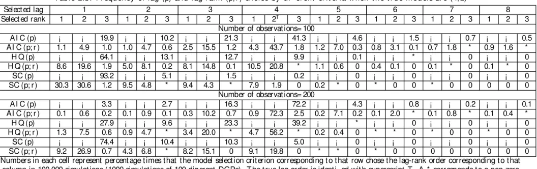
Table 2.a shows t he frequency of lag-order select ion in 1000 simulat ions of 100 t rivariat e
VARs(4) wit h rank 1 by AIC, HQ and SC when only full rank models are considered, and
when rank and lag orders are det ermined simult aneously. T he t op half of t his t able
corre-sponds t o a sample size of 100, and t he bot t om half correcorre-sponds to samples of 200
observa-t ions. Table 2.b shows observa-t he analogous frequencies when observa-t he observa-t rue DGP is a observa-t rivariaobserva-t e VAR(4)
of rank 2.
These Tables con…rm t hat select ing t he lag and rank order joint ly, can lead t o choice of a
model which is of higher lag-order t han t he lag-lengt h chosen when only full rank models are
considered. For example, t he t op half of Table 2.a shows t hat for samples of 100 observat ions,
t he modal choice of all t hree crit eria is VAR(1), wit h AI C choosing t he t rue lag of 4 only
14 percent of t he t ime. The ot her two criteria choose a VAR(4) wit h a frequency of less
t han 1 percent . However, when t he lag and rank are chosen simult aneously, t here is a large
reduct ion in t he number of t imes t hat t he VAR(1) is chosen, regardless of t he crit erium used.
Furt hermore, t he frequency of t he correct lag chosen increases signi…cant ly. In bot h Tables
wit hH Q a close second. The modal choice of t he Schwarz crit erium st ays at a VAR(1) even
wit h 200 observat ions.
Two point s are worth noting. First , even in t hose cases in which t he crit eria choose
t he wrong lag-lengt h, t hey are likely t o choose t he correct rank. The only except ion isSC
when t he t rue rank is 2 and t here are only 100 observat ions. This suggest s t hat common
cycles can be det ect ed even if t he wrong lag-lengt h is chosen. This is plausible, because
t he property t hat a linear combinat ion of variables has no dependence wit h t he past (t he
necessary and su¢ cient condit ion for common cycles), is unrelat ed t o what t hose cycles are
and whet her t hey are correct ly speci…ed. The second point is t hat AI C has a t endency t o
over-predict t he t rue lag lengt h, even when sample size is 200, once one chooses lag-lengt h
and rank simult aneously. Given t he evidence on t he adverse e¤ect s of overparamet erizat ion
on forecast ing in t ime series models in t he lit erat ure (see Lüt kepohl, 1985), t his caut ions us
t hat t he cost s of usingAI C t o choose lag and rank order joint ly may outweigh it s bene…ts.
The analysis of t he forecast s in t he next subsect ion con…rms t hat t his is indeed t he case.
4.2. For ecast s
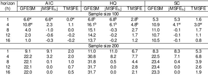
Tables 3.a and 3.b show t he percent age improvement in t hese measures when lag and rank
are chosen simult aneously, over when lag-lengt h is chosen alone imposingr = n. A general
conclusion is t hat reduced-rank models have no forecast ability beyond 8 periods, and most
of t he advant age of looking for common cycles is in forecast ing one t o four periods ahead.
Despit e t hat , t here are st ill non-t rivial gains for considering t he possibility of reduced-rank
models: GF E SM can be reduced up t o 32%, jM SF Ehj up t o 11% and TM SF E up t o 8%,
when t he t rue rank is one. For rank two t hese pot ent ial reduct ions are respect ively 31%, 9%,
and 5%. These numbers are about half as large as our benchmark case when GF E SM and
jM SF Ehj are considered, but are larger when TM SF E is considered.
The result s in Tables 3.a and 3.b allow also comparing t he t hree informat ion crit eria in
provides t he best forecast ing performance across informat ion crit eria, whileAI C provides t he
worst . Our result s for H Q and SC show t hat t here are sizable bene…ts from choosing lag
and rank joint ly. In t hese cases, t hese crit eria give rise t o models t hat are closer t o t he t rue
DGP, wit hout increasing t he chance of overshoot ing t he correct lag.
On t he ot her hand, considering t he forecast performance of AI C, and t he increased
possibility of over-predict ion of t he lag-order when lag and rank are chosen simult aneously,
especially when sample size is 100, we conclude t hat t he joint det erminat ion of lag and order
byAI Cin models wit h small R2is not appropriat e. Indeed, if one want s t o useAI C, and also
want s t o allow for possibility of common cycles, it would be bet t er t o employ t he following
st rategy. First , useAI C t o choose t he lag lengt h t est ing for common cycles using t he test in
Vahid and Engle(1993). Then, impose common cycles if t hat is not reject ed by t he t est ing
procedure. In t his way, t he possibility of overshoot ing t he correct lag lengt h is somewhat
cont rolled.
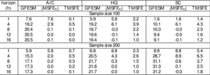
4.3. Var iance-decom p osit i on r esul t s
The percent improvement of est imat es of forecast -error variance decomposit ion coe¢ cient s
are present ed in Table 4. First not ice t hat t he smallest gains (largest losses) are obt ained
for horizon one, where result s depend exclusively on t he est imat e of t he variance-covariance
mat rix of t he errors12; a similar result is obt ained in our benchmark case. This may be due
t o t he fact t hat t he variance cont ribut ions are a rat io of element s of t he variance-covariance
mat rix. Hence, alt hough t he rest rict ed model est imat es t he lat t er more precisely, it performs
worse in est imat ing t he variance rat ios compared t o t he unrest rict ed model. Second, when
sample size is 100 observat ions, t here is no consist ent pat t ern of result s favoring
reduced-rank crit eria (i.e., when lag and reduced-rank are joint ly select ed). Third, increasing t he sample size
t o 200 observat ions improves t he gains of reduced-rank models regardless of t he crit erium
considered. The highest realized gain happens when t heH Q crit erium is used in t his case,
12Not ice t hat , for horizon one, when t he Choleski decomposit ion is employed, t here are only …ve variance
alt hough t his says not hing about t he relat ive performance across crit eria for est imat ion of
variance-decomposit ion est imat es.
5. M ont e-Car lo simulat ion r esult s for t he six-var iable m odel
The DGPs of t he six-variable Mont e-Carlo simulat ions are drawn uniformly from t he
con-…dence region of an est imat ed six-variable VAR(2) of rank 4, based on US macroeconomic
aggregates. T he six variables are t he growt h rat es of per-capit a income, consumpt ion,
in-vest ment and real money balances, and t he …rst di¤erence of int erest rat es and t he in‡at ion
rat e, from 1947:1 t o 1988:4. This is t he dat a set used in King, et al(1991). The addit ion
of t he monet ary variables t o t he syst em, increases t he syst em R2 from 0.44 to 0.81. This is
possibly due t o t he fact t hat monet ary variables are more dependent on t he past t han real
variables, and t hat t here is a st rong cross correlat ion between t he growt h rat es of real money
balances and income.
The maximum lag-lengt h considered is 6, which is t he lag lengt h t hat King et al.(1991)
used in t heir analysis. In order t o reduce t he comput at ional cost s, we have drawn only 20
DGPs and performed 500 simulat ions in each case. In cont rast t o t he t hree-variable model,
t he DGPs in t his exercise all haveR2 between 0:8and 0:9;which implies t hat …nit e samples
are more informat ive about t he st ruct ure of t he DGP t han in t he previous t hree variable
case, and t hat informat ion crit eria must be more successful in select ing t he correct lag. This
is clear from t he lag and lag-rank orders chosen by t he di¤erent crit eria report ed in Table 5.
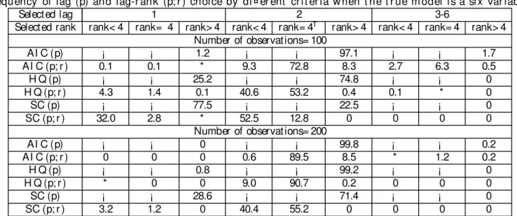
Table 5 shows t he frequency of making t he correct choice, using each of the t hree crit eria.
The problem wit h AI C over-shoot ing t he correct lag, when lag and rank order is chosen
simult aneously, is much more pronounced here, especially in samples of 100 observat ions.
In t his case, t he regular AI C only overshoot s t he t rue lag-order in less t han 2 percent , but
t he lag-rank version of t heAI C overshoot s the t rue lag in 9.4 percent of all of t he 10,000
simulat ions. If we add t he 8.3 percent age of t imes t hat AI C overpredict s t he rank even
model in more t han 17 percent in all simulat ions.
The int erest ing informat ion in Table 5, however, is t he relative success of t he
Hannan-Quinn crit erium in choosing t he correct lag and rank order, wit hout t he risk of
overpa-ramet erizing t he model. T his repeat s what we observed in our t hree-variable simulat ions.
Even wit h a sample size of 100, the Hannan-Quinn crit erium chooses t he correct lag 94.2
percent of t he t imes, and leads t o overparamet erized models in less than 0.5 percent of all
simulat ions. Wit h a sample size of 200, t he Hannan-Quinn crit erium is almost perfect in
choosing t he correct lag-order (99.98 percent ), and is t he best among t he t hree crit eria for
choosing t he correct lag-rank combination 90.7 percent in all simulat ions. Alt hough t he
per-cent age of t he t imes t hat t he Schwarz crit erium chooses t he true lag improves when t he lag
and rank order are chosen simult aneously, t his crit erium is st ill signi…cant ly biased t owards
under-paramet erizing t he model, even when t he signal is st rong and t he sample size is 200.
The confusion caused byAI C when it is used t o choose lag and rank order simult aneously,
is re‡ect ed in its forecast performance. Table 6 shows t he improvement in t he forecast ing
performance of models chosen by t he di¤erent crit eria when rank order is chosen in t he model
select ion st age over when it is ignored. When t he sample size is 100, usingAI C t o choose
t he lag-lengt h and rank order simult aneously leads t o very poor forecast performance of t he
select ed model, for longer t han one st ep ahead horizons. Given t he relat ive success of t he
Hannan-Quinn crit erium in choosing t he correct lag-rank order, it leads t o models wit h t he
best overall forecast performance, withAI C being a close second only when t he sample size
is 200. Unlike t he case where t he signal t o noise rat io was small, t he underparamet erizat ion
of t he t rue model by t he Schwarz crit erium is re‡ect ed by a very poor relat ive forecast
performance of models chosen by t his crit erium.
6. Conclusions
This paper argues t hat t he stylized fact t hat “ macroeconomic variables move t oget her over
a VAR or a VEC model. The Mont e-Carlo analysis in t his paper suggest s the following
messages t o pract it ioners who analyze dat a which exhibit comovement :
1. There are non-t rivial gains in forecast ing accuracy and in MSE of est imat es of
variance-decomposit ion coe¢ cient s when we allow VAR and VEC models t o be of reduced rank.
These result s are st ronger in our benchmark case (lag order is known), but are con…rmed
as well for t he more realist ic case where lag order is select ed using popular informat ion
crit eria.
2. Informat ion crit eria t hat allow for reduced-rank VAR and VEC models perform bet t er
in choosing t he correct lag lengt h compared t o t hese same informat ion crit eria t hat
disregard reduced-rank models(n = r ).
3. If H Q and SC are used in a cont ext which allows t hem t o pick reduced rank models,
t hen t he problem t hat t hey underpredict t he t rue lag-lengt h is signi…cant ly remedied.
4. Do not useAI C t o choose lag and rank order at t he same t ime, especially when t he
sample size is small.
5. The Hannan-Quinn crit erium seems t o be t he best crit erium for choosing lag-lengt h
and rank order at t he same t ime.
The analysis also con…rms t hat AI C can lead t o over-paramet erized models wit h adverse
consequences for forecast performance. However, it reveals t hat Lüt kepohl’s(1985) conclusion
t hat models select ed by Schwarz crit erium lead t o best forecast s is an art ifact of his Mont
e-Carlo design.
R efer ences
Ahn, S. K. and G. C. Reinsel(1988), “ Nest ed reduced-rank aut oregressive models for
Beveridge, S. and Nelson, C.R.(1981), “ A New Approach t o Decomposit ion of Economic
Time Series int o a Permanent and Transit ory Component s wit h Part icular At t ent ion
t o Measurement of t he “ Business Cycle” , Journal of Monetary Economics, vol. 7, pp.
151-174.
Carlino, G. and K. Sill(1998), “ Common t rends and common cycles in regional per-capit a
incomes” , Working Paper, Federal Reserve Bank of Philadelphia.
Clement s, M. P. and D. F. Hendry(1995), “ Forecast ing in cointegrat ed syst ems” , Journal
of Applied Econometrics, 10, 127-146.
Clement s, M. P. and D. F. Hendry(1994), “ Towards a t heory of economic forecast ing” ,
Chapt er 2 in C. P. Hargreaves (Ed.), Nonstationary Time Series Analysis and
Cointe-gration, Oxford University Press.
Engle, R. F. and S. J. Brown(1986), “ Model select ion for forecast ing” , Applied Mathematics
and Computation, 20, 313-327.
Engle, R. F. and C. W. J. Granger(1987), “ Coint egrat ion and error correct ion:
Represen-t aRepresen-t ion, esRepresen-t imaRepresen-t ion and Represen-tesRepresen-t ing” , EconomeRepresen-trica, 55, 251-276.
Engle, R. F. and J. V. Issler(1995), “ Est imat ing common sect oral cycles” , Journal of
Monetary Economics, 35, 83-113.
Engle, R.F. and S. Yoo(1987), “ Forecast ing and t est ing in coint egrat ed syst ems” , Journal
of Econometrics, 35, 143-159.
Granger, C. W. J., M. L. King and H. Whit e(1995), “ Comment s on t est ing economic
t heories and t he use of model select ion crit eria” , Journal of Econometrics, 67, 173-187.
Hamilt on, J. D.(1994), Time Series Analysis, Princet on University Press.
King, R., C. I. Plosser, J. H. St ock and M. W. Wat son(1991), “ St ochast ic Trends and
King, R.G., Plosser, C.I. and Rebelo, S.(1988), “ Product ion, Growt h and Business Cycles.
I I. New Direct ions,” Journal of Monetary Economics, vol. 21, pp. 309-341.
Issler, J.V. and Ferreira, P.C.(1998), “ Time-Series propert ies and empirical evidence of
growt h and infrast ruct ure,” Working Paper # 335, Graduat e School of Economics,
Get ulio Vargas Foundation.
Issler, J.V. and Vahid, F.(1998), “ Common cycles and t he import ance of t ransit ory shocks
t o macroeconomic aggregat es,” Working Paper # 334, Graduat e School of Economics,
Get ulio Vargas Foundation.
Lin, J. L. and R. S. Tsay(1996), “ Coint egrat ion const raint s and forecast ing: An empirical
examinat ion” , Journal of Applied Econometrics, 11, 519-538.
Lucas, R. E. Jr.(1977), “ Underst anding business cycles” , Carnegie-Rochester Series on
Public Policy, 5, 7-29, also reprint ed in Lucas, R. E. Jr. (Ed) Models of Business Cycle,
1977.
Lüt kepohl, H.(1993), Introduction to Multiple Time Series Analysis, Second Edit ion,
Springer-Verlag.
Lüt kepohl, H.(1985), “ Comparison of crit eria for est imat ing t he order of a vect or aut
ore-gressive process” , Journal of Time Series Analysis, 6, 35-52.
Magnus, J. R. and H. Neudecker(1988), Matrix Di¤erential Calculus with Applications in
Statistics and Econometrics, John Wiley.
Neusser, Klaus(1991). “ Testing t he Long-Run Implicat ions of t he Neoclassical Growt h
Model,” Journal of Monetary Economics, v27(1), 3-38.
Nickelsburg, G.(1982), “ Small sample propert ies of dimensionality st at ist ics for …tt ing VAR
models t o aggregat e economic dat a: A Mont e Carlo st udy” , Proceedings of the Business
Reinsel, G. C.(1993), Elements of Multivariate Time Series Analysis, Springer-Verlag.
St ock, J. H. and M. W. Wat son(1988), “ Test ing for common t rends” , Journal of the
Amer-ican Statistical Association, 83, 1097-1107.
Toda, Hiro Y. and Pet er C. B. Phillips(1993), “ Vector Aut oregressions and Causality,”
Econometrica, vol. 61(6), pp. 1367-1393.
Tiao, G. C. and R. S. Tsay(1989), “ Model speci…cat ion in mult ivariat e time series (wit h
discussion)” , Journal of the Royal Statistical Society, Series B, 51, 157-213.
Tso, M.K.-S.(1981), “ Reduced rank regression and Canonical analysis” Journal of the
Royal Statistical Society, Series B, 43, 183-189.
Vahid, F. and R. F. Engle(1993), “ Common t rends and common cycles” , Journal of Applied
Econometrics, 8, 341-360.
Velu, R. P., G. C. Reinsel and D. W. Wickern(1986), “ Reduced rank models for mult iple
t ime series” , Biometrika, 73, 105-118.
A . Sy st em R
2and signal-t o-noise r at io
In a mult iple regression wit h st ochast ic regressors and i.i.d. errors,y = X ¯ + " ;t he limit ing
signal-t o-noise ratio(snr ) can be de…ned as:
snr = ¯
0lim T ! 1 E
³
X0X
T
´
¯ ¾2
"
; (A.1)
whereE (" "0) = ¾2
" ¢I, and t he proport ion of t he variat ion of dependent variable explained
by t he model, i.e. t he populat ionR2, is:
R2= ¯
0
limT ! 1 E
³
X0X
T
´
¯
¾2 " + ¯
0
limT ! 1 E
³
X0X
T
´
¯ =
Since t he asympt ot ic variance ofpT³¯b¡ ¯´ isAV AR(¯ ) = ¾b 2 "
³
limT ! 1 E
³
X0X
T
´ ´¡ 1
, we
can writ e (A.1) as:
snr = ¯0³AV AR(¯ )b ´¡ 1¯ : (A.2)
Consider now aV AR(p):
yt = A1yt¡ 1+ ¢¢¢+ Apyt ¡ p+ "t: (A.3)
The analogous measure of snr for it is:
snr = ¯0³§ - - ¡ 1´ ¯ (A.4)
where¯ = vec(A),A =
·
A1 : : : Ap
¸
, E³"t"0t ¡ j
´
= - , and:
§ = 0 B B B B B B B B @
¡ 0 ¡1 ¢¢¢ ¡p¡ 1
¡ 0
1 ¡0 ¢¢¢ ¡p¡ 2
¢¢¢ ¢¢¢ ¢¢¢ ¢¢¢
¡0
p¡ 1 ¡ 0p¡ 2 ¢¢¢ ¡0
1 C C C C C C C C A ;
where¡j = E
³
ytyt ¡ j0
´
:Notice t hat § is complet ely det ermined by(A; - )via t he Yule-Walker
equat ions13. Aft er some algebra, it can be shown t hat (A.4) is equal t o:
snr = ¯0³§ - - ¡ 1´ ¯ = tr ace³¡ 0- ¡ 1
´
¡ n:
Using t his last result , one can t hen de…ne the syst em R2t o be:
R2= tr ace(¡ 0
-¡ 1)¡ n
1 + tr ace(¡ 0- ¡ 1)¡ n
:
Table 1: Per cent age im pr ovem ent i n M SE of for ecast -er r or var iance decomp osit ions, and di¤ er ent for ecast m easur es w hen t he l ag lengt h is know n
horizon True rank is one True rank is two
(h) GFESM jMSFEhj T MSFE Var. Dec. GFESM jMSFEhj T MSFE Var. Dec.
Sample size 100
1 22.22 22.22 1.97 -14.10 12.08 12.08 0.98 -39.60 4 60.41 8.66 1.72 45.55 34.56 5.02 0.96 45.23 8 70.54 1.70 1.39 46.91 42.57 1.32 0.77 43.84 12 72.34 0.46 1.03 46.25 44.66 0.45 0.59 46.91 16 72.86 0.21 0.81 45.95 45.26 0.25 0.47 47.73
Sample size 200
T abl e 2.a: Fr equency of l ag (p) and lag-r ank (p; r ) choice by di¤ er ent cr it er i a when t he t r ue m odels ar e (4; 1)
Select ed lag 1 2 3 4 5 6 7 8
Select ed rank 1 2 3 1 2 3 1 2 3 1T 2 3 1 2 3 1 2 3 1 2 3 1 2 3
Number of observat ions= 100
AI C (p) ¡ ¡ 57.0 ¡ ¡ 13.1 ¡ ¡ 12.6 ¡ ¡ 14.0 ¡ ¡ 2.0 ¡ ¡ 0.7 ¡ ¡ 0.3 ¡ ¡ 0.3 AI C (p; r ) 10.8 2.5 0.4 7.4 2.0 0.1 14.4 2.4 0.1 32.7 3.4 * 8.3 1.1 * 5.0 0.6 * 3.8 0.4 * 4.0 0.5 *
H Q (p) ¡ ¡ 92.9 ¡ ¡ 4.7 ¡ ¡ 1.7 ¡ ¡ 0.7 ¡ ¡ * ¡ ¡ * ¡ ¡ 0 ¡ ¡ 0 H Q (p; r ) 39.2 1.9 0.2 13.3 0.3 * 17.0 0.1 * 24.3 0.1 * 2.4 * 0 0.7 * 0 0.3 0 0 0.1 0 0 SC (p) ¡ ¡ 99.6 ¡ ¡ 0.4 ¡ ¡ * ¡ ¡ * ¡ ¡ 0 ¡ ¡ 0 ¡ ¡ 0 ¡ ¡ 0 SC (p; r ) 73.8 0.4 * 10.7 * 0 8.4 0 0 6.6 0 0 0.1 0 0 * 0 0 0 0 0 0 0 0
Number of observat ions= 200
AI C (p) ¡ ¡ 25.9 ¡ ¡ 10.7 ¡ ¡ 20.0 ¡ ¡ 40.0 ¡ ¡ 2.7 ¡ ¡ 0.5 ¡ ¡ 0.2 ¡ ¡ * AI C (p; r ) 2.2 0.7 0.1 3.3 0.8 * 12.1 1.8 * 56.4 4.1 0.1 9.1 0.8 * 4.1 0.3 0 2.3 0.1 0 1.6 0.1 0 H Q (p) ¡ ¡ 80.1 ¡ ¡ 7.8 ¡ ¡ 7.2 ¡ ¡ 4.9 ¡ ¡ * ¡ ¡ 0 ¡ ¡ 0 ¡ ¡ 0 H Q (p; r ) 16.1 0.6 0.1 8.9 0.1 * 20.7 0.1 0 51.3 * 0 1.9 0 0 0.2 0 0 * 0 0 * 0 0 SC (p) ¡ ¡ 98.6 ¡ ¡ 1.0 ¡ ¡ 0.3 ¡ ¡ 0.1 ¡ ¡ 0 ¡ ¡ 0 ¡ ¡ 0 ¡ ¡ 0 SC (p; r ) 49.4 0.1 * 11.1 * 0 17.1 0 0 22.3 0 0 0.1 0 0 * 0 0 0 0 0 0 0 0 Numbers in each cell represent percent age t imes t hat t he model select ion crit erion corresponding t o t hat row chose t he lag-rank order corresponding t o t hat
Table 2.b: Fr equency of lag (p) and l ag-r ank (p; r ) choice by di¤ er ent cr it er ia w hen t he t r ue m odel s ar e (4; 2)
Select ed lag 1 2 3 4 5 6 7 8
Select ed rank 1 2 3 1 2 3 1 2 3 1 2T 3 1 2 3 1 2 3 1 2 3 1 2 3
Number of observat ions= 100
AI C (p) ¡ ¡ 19.9 ¡ ¡ 10.2 ¡ ¡ 21.3 ¡ ¡ 41.3 ¡ ¡ 4.6 ¡ ¡ 1.5 ¡ ¡ 0.7 ¡ ¡ 0.5 AI C (p; r ) 1.1 4.9 1.0 1.0 4.7 0.6 2.5 15.5 1.2 4.3 43.7 1.8 1.2 7.0 0.3 0.8 3.1 0.1 0.7 1.8 * 0.9 1.6 *
H Q (p) ¡ ¡ 64.1 ¡ ¡ 13.1 ¡ ¡ 12.7 ¡ ¡ 9.9 ¡ ¡ 0.1 ¡ ¡ * ¡ ¡ 0 ¡ ¡ 0 H Q (p; r ) 8.6 19.6 1.9 5.0 8.1 0.2 8.1 14.8 0.1 10.5 20.8 * 1.1 0.6 0 0.4 0.1 0 0.1 * 0 0.1 * 0 SC (p) ¡ ¡ 93.2 ¡ ¡ 5.1 ¡ ¡ 1.5 ¡ ¡ 0.2 ¡ ¡ 0 ¡ ¡ 0 ¡ ¡ 0 ¡ ¡ 0 SC (p; r ) 30.3 30.6 1.2 9.5 4.8 * 9.4 4.3 * 7.9 1.9 0 0.2 * 0 * 0 0 * 0 0 0 0 0
Number of observat ions= 200
AI C (p) ¡ ¡ 3.3 ¡ ¡ 2.7 ¡ ¡ 16.3 ¡ ¡ 72.2 ¡ ¡ 4.3 ¡ ¡ 0.8 ¡ ¡ 0.2 ¡ ¡ 0.1 AI C (p; r ) 0.1 0.6 0.2 0.1 0.9 0.1 0.3 10.2 0.7 0.9 72.3 2.5 0.2 7.1 0.2 0.1 2.0 * 0.1 0.8 * 0.1 0.4 *
H Q (p) ¡ ¡ 27.9 ¡ ¡ 9.6 ¡ ¡ 23.3 ¡ ¡ 39.2 ¡ ¡ * ¡ ¡ 0 ¡ ¡ 0 ¡ ¡ 0 H Q (p; r ) 1.3 7.5 0.6 0.9 4.7 * 3.4 20.0 * 4.7 56.2 * 0.2 0.4 0 * * 0 * 0 0 * 0 0 SC (p) ¡ ¡ 74.4 ¡ ¡ 10.4 ¡ ¡ 10.3 ¡ ¡ 5.0 ¡ ¡ 0 ¡ ¡ 0 ¡ ¡ 0 ¡ ¡ 0 SC (p; r ) 9.2 26.9 0.7 4.3 6.8 * 8.2 15.1 0 9.1 19.8 0 * * 0 * 0 0 0 0 0 0 0 0 Numbers in each cell represent percent age t imes t hat t he model select ion crit erion corresponding t o t hat row chose t he lag-rank order corresponding t o t hat