❊♥s❛✐♦s ❊❝♦♥ô♠✐❝♦s
❊s❝♦❧❛ ❞❡
Pós✲●r❛❞✉❛çã♦
❡♠ ❊❝♦♥♦♠✐❛
❞❛ ❋✉♥❞❛çã♦
●❡t✉❧✐♦ ❱❛r❣❛s
◆◦ ✹✶✼ ■❙❙◆ ✵✶✵✹✲✽✾✶✵
❚❤❡ ■♠♣♦rt❛♥❝❡ ♦❢ ❈♦♠♠♦♥ ❈②❝❧✐❝❛❧ ❋❡❛✲
t✉r❡s ✐♥ ❱❆❘ ❆♥❛❧②s✐s✿ ❆ ▼♦♥t❡✲❈❛r❧♦ ❙t✉❞②
❋❛rs❤✐❞ ❱❛❤✐❞✱ ❏♦ã♦ ❱✐❝t♦r ■ss❧❡r
❖s ❛rt✐❣♦s ♣✉❜❧✐❝❛❞♦s sã♦ ❞❡ ✐♥t❡✐r❛ r❡s♣♦♥s❛❜✐❧✐❞❛❞❡ ❞❡ s❡✉s ❛✉t♦r❡s✳ ❆s
♦♣✐♥✐õ❡s ♥❡❧❡s ❡♠✐t✐❞❛s ♥ã♦ ❡①♣r✐♠❡♠✱ ♥❡❝❡ss❛r✐❛♠❡♥t❡✱ ♦ ♣♦♥t♦ ❞❡ ✈✐st❛ ❞❛
❋✉♥❞❛çã♦ ●❡t✉❧✐♦ ❱❛r❣❛s✳
❊❙❈❖▲❆ ❉❊ PÓ❙✲●❘❆❉❯❆➬➹❖ ❊▼ ❊❈❖◆❖▼■❆ ❉✐r❡t♦r ●❡r❛❧✿ ❘❡♥❛t♦ ❋r❛❣❡❧❧✐ ❈❛r❞♦s♦
❉✐r❡t♦r ❞❡ ❊♥s✐♥♦✿ ▲✉✐s ❍❡♥r✐q✉❡ ❇❡rt♦❧✐♥♦ ❇r❛✐❞♦ ❉✐r❡t♦r ❞❡ P❡sq✉✐s❛✿ ❏♦ã♦ ❱✐❝t♦r ■ss❧❡r
❉✐r❡t♦r ❞❡ P✉❜❧✐❝❛çõ❡s ❈✐❡♥tí✜❝❛s✿ ❘✐❝❛r❞♦ ❞❡ ❖❧✐✈❡✐r❛ ❈❛✈❛❧❝❛♥t✐
❱❛❤✐❞✱ ❋❛rs❤✐❞
❚❤❡ ■♠♣♦rt❛♥❝❡ ♦❢ ❈♦♠♠♦♥ ❈②❝❧✐❝❛❧ ❋❡❛t✉r❡s ✐♥ ❱❆❘ ❆♥❛❧②s✐s✿ ❆ ▼♦♥t❡✲❈❛r❧♦ ❙t✉❞②✴ ❋❛rs❤✐❞ ❱❛❤✐❞✱ ❏♦ã♦ ❱✐❝t♦r ■ss❧❡r ✕ ❘✐♦ ❞❡ ❏❛♥❡✐r♦ ✿ ❋●❱✱❊P●❊✱ ✷✵✶✵
✭❊♥s❛✐♦s ❊❝♦♥ô♠✐❝♦s❀ ✹✶✼✮
■♥❝❧✉✐ ❜✐❜❧✐♦❣r❛❢✐❛✳
The Importance of Common Cyclical Features in VAR Analysis:
A Monte-Carlo Study
∗
Farshid Vahid
†Department of Econometrics and Business Statistics
Monash University
Clayton, Victoria 3800
Australia
[email protected]
João Victor Issler
Graduate School of Economics — EPGE
Getulio Vargas Foundation
Praia de Botafogo 190 s. 1111
Rio de Janeiro, RJ 22253-900
Brazil
[email protected]
First version: November 1999
Revised: March 2001
A bst r act
Despite the commonly held belief that aggregate data display short-run comovement, there has been little discussion about the econometric consequences of this feature of the data. We use exhaustive Monte-Carlo simulations to investigate the importance of restrictions implied
∗A ck now l edgm ent s: This paper was written while João Victor Issler was visiting Monash University, and it was revised while Farshid Vahid was visiting Getulio Vargas Foundation. The hospitality of both institutions are gratefully acknowledged. We have beneÞted from comments and suggestions of Heather Anderson, Carlos Martins-Filho, Aman Ullah, Arnold Zellner (Editor), the Associate Editor, four anonymous referees, and participants of the Latin American and the European Meetings of the Econometric Society. We thank George Athanasopoulos for excellent research assistance. The authors are responsible for any remaining errors in this paper. João Victor Issler acknowledges the support of CNPq-Brazil and PRONEX. Farshid Vahid is grateful forÞnancial support provided by the Monash University Research Fund Grant No. 22.097.007, and CNPq-Brazil.
†
by common-cyclical features for estimates and forecasts based on vector autoregressive models. First, we show that the “best” empirical model developed without common cycle restrictions need not nest the “best” model developed with those restrictions. This is due to possible differences in the lag-lengths chosen by model selection criteria for the two alternative models. Second, we show that the costs of ignoring common cyclical features in vector autoregressive modelling can be high, both in terms of forecast accuracy and efficient estimation of variance decomposition coefficients. Third, weÞnd that the Hannan-Quinn criterion performs best among model selection criteria in simultaneously selecting the lag-length and rank of vector autoregressions.
K ey wor ds: Reduced rank models, model selection criteria, forecasting, variance decomposition.
JEL C lassifi cat ion: C32, C53.
1. I nt r oduct ion
In this paper we argue that short-run dynamic restrictions should be taken seriously in vector autoregressive (VAR) modelling. We focus on common-cycle restrictions because of their importance in macroeconomics. Common cyclical movements in detrended economic variables have been so prevalent that they have acquired the status of “stylized facts.” Lucas (1977) states that the main regularities observed in cyclical ßuctuations of economic time series are in their comovement. In empirical studies, common cycles have been shown to be a feature of a variety of macroeconomic data sets. For example, Campbell and Mankiw (1989) Þnd a common cycle between consumption and income for most G-7 countries. Engle and Kozicki (1993) Þnd common international cycles in GNP data for OECD countries. Using US data, Issler and Vahid (2001) Þnd common cycles for macroeconomic aggregates, and Engle and Issler (1995) and Carlino and Sill (1998) Þnd common cycles for sectoral and regional outputs respectively. Like most applied macroeconomic research in the last Þfteen years, these studies have investigated common-cyclical features using vector-autoregressive (VAR) or vector error-correction (VEC) models.
are generally most useful for forecasting over short horizons. Hence, imposing short-run constraints might be a way of improving the effectiveness of time-series models at horizons where they are most useful.
Incorporating common-cycle restrictions can reduce the number of free parameters of a VAR model and help achieve parsimony, more than cointegrating restrictions can. For example, when dealing with post-war quarterly data, and a VAR with three variables and eight lags, there are seventyÞve mean parameters to be estimated from about two hundred data points on each variable. If the three-variable system has one known cointegrating vector, the number of free parameters falls from seventyÞve to sixty nine when estimating a VEC model. Common-cyclical features show more potential in reducing the number of conditional-mean parameters. If the three variables in the VEC model share one common cycle, then the number of mean parameters falls from sixty nine to twenty seven.
We assess the effects of common-cyclical features on VAR models using Monte-Carlo simulations. The focus here is on the accuracy of multi-step ahead out-of-sample forecasts, as well as the accuracy of estimates of impulse-response functions and variance-decomposition of forecast errors. We design the simulations so that the results would be relevant for an applied macroeconomist estimating a relatively large number of parameters using a limited number of data points. To that end, we consider a variety of Data Generating Processes (DGPs) and sample sizes, that are similar to the “typical” data sets that applied researchers encounter in practice.
VAR models with common cycles fall into the general category of reduced-rank multivariate models1. We can represent these models in a reduced-rank regression framework by zt=Φxt+εt, where zt contain the n-series of interest, xt contains p lags of zt (and possibly error-correction terms), and εt is a multivariate white-noise process. The matrix Φ is not full rank, reßecting the fact that there are linear combinations of zt that are white noise. If common cycles are a true feature of the data, and if the lag order of the VAR (VEC) is known to be p, then theory tells us that the estimate of Φ with the correct rank-restrictions imposed must be more efficient than the unrestricted estimate of Φ(see Ahn and Reinsel 1988). Even so, researchers may be reluctant to incorporate these parameter restrictions because of the asymmetric consequences of over versus under-parametrization. Because the true rank of Φ is not known, it may seem wiser to live with a possibly inefficient unconstrained model rather than with a misspeciÞed inconsistent model. We argue here that the cost of ignoring common-cycle restrictions is more than the efficiency loss in estimating Φ. We show that, if only full-rank models are considered, the lag length chosen by the usual model-selection criteria is severely misspeciÞed. Standard criteria may Þnd too small a lag length in reduced-rank VARs simply because this is the only possible way available to achieve 1Classic references on reduced-rank VAR’s include Velu, Reinsel and Wickern (1986), Ahn and Reinsel (1988), and
parsimony. For such misspeciÞed models one cannot tell from theory what the consequences of incorporating rank restrictions will be.
An alternative to the usual model-selection criteria is to choose the lag length and the rank of the VAR simultaneously. Lütkepohl (1993, page 202) presents a set of model-selection criteria that can be used for that purpose, and we refer to this set as IC(p, r). Our simulations reveal that, when the true DGP is a reduced-rank VAR model, the lag length chosen by the standard model-selection criteria (which we refer to as IC(p)) can be quite different from that chosen when rank and order are selected simultaneously. Standard model-selection criteria that place a strong penalty on over-parameterization, such as the Schwarz or Hannan-Quinn criteria, may choose too small a lag-length when the true model has common cycles. However, they improve if the rank order is simultaneously selected with the lag length. We Þnd strong evidence in favor of Hannan-Quinn criterion for choosing the correct lag and rank order overall. Regarding the Akaike information criterion, we observe that its tendency to choose an over-parameterized model when the lag order and rank are selected simultaneously is accentuated relative to the case when only the lag length is selected.
Users of VAR models are often interested in forecasts, rather than the true lag order. Hence, we compare models based on their forecasting accuracy measures. For horizons up to sixteen periods ahead, using several measures of forecasting accuracy, we Þnd that the forecasts produced by the reduced-rank models selected by IC(p, r) are generally superior to those produced by the models selected by IC(p). Indeed, on average, if the Hannan-Quinn criterion is used to select lag order and rank, the cumulative accuracy of one to four-step-ahead forecasts can be improved by up to 20%. This sizable effect illustrates the potential gain associated with considering common-cycle restrictions at the model selection stage. For variance decompositions, reduced-rank models selected by IC(p, r) only do better when samples are large (more than 200 observations)2.
The outline of the paper is as follows. Section 2 states the reduced-rank restrictions that common cyclical ßuctuations impose on the parameters of VAR models, and presents the model-selection criteria for reduced-rank models. Section 3 describes our Monte-Carlo design. Section 4 presents the simulation results. Section 5 presents a small empirical example using coincident and leading business-cycle series. Finally, Section 6 presents the main conclusions of the paper, as well as a suggestion for further research.
2
2. Com m on cycles in VA R m odels
As in most applied macroeconomic research, we assume that the objective is to build a time series model for the growth rate of a vector of n economic variables. We denote the levels of these variables at time t by Yt, their logarithms byyt, and their growth rates (i.e. the Þrst difference of the logarithm of Yt) by ∆yt. We make the reasonable assumption that ∆yt is stationary, add the simplifying assumption that∆yt has mean zero (without any loss of generality), and start with the Wold representation of∆yt, i.e.
∆yt=C(L)εt, (2.1)
whereC(L) = ∞
j= 0CjLj is a matrix polynomial in the lag operator andC0=In. From the work of Beveridge and Nelson (1981) and Stock and Watson (1988), it is possible to decompose the log-level series yt into common trends and cycles (we refer to this as the Beveridge-Nelson-Stock-Watson — or BNSW — decomposition). Using the identityC(L) =C(1) +∆C∗
(L), ignoring the initial value of y0, and integrating both sides of (2.1) we get3:
yt = C(1) t
j= 1
εj+C∗(L)εt
= τt+ct, (2.2)
where τt = C(1) tj= 1εj and ct = C∗(L)εt represent the trend and cyclical components of yt respectively. In the BNSW decomposition, the n variables in yt are decomposed into n random-walk components (stochastic trends) and nstationary components (stochastic cycles). IfC(1) has rankn−q(q >0), the stochastic trends inytcan be characterized as linear combinations of onlyn−q common random walks, in which case yt is said to be cointegrated, or to have common stochastic trends, withq linearly independent cointegrating vectors (see Engle and Granger, 1987). IfC∗
(L) has rankr (r < n), then the stochastic cycles inyt can be characterized as linear combinations ofr common stochastic cycles, with n−r linearly independent cofeature vectors (see Vahid and Engle, 1993). In this paper, we investigate the costs of ignoring this singularity in the stochastic cyclesct.
For ease of exposition we assume that there is no cointegration in the system (q= 0)4, in which case the appropriate model for ∆yt will be a VAR, i.e.,
∆yt = A1∆yt−1+...+Ap∆yt−p+εt
= A1 . . . Ap
∆yt−1
.. .
∆yt−p
+εt
3
See Stock and Watson (1988) or Vahid and Engle (1993) for more details.
4If there is cointegration, then the appropriate error-correction term has to be added to the right-hand side of
= Φxt+εt, (2.3)
whereΦ= A1 . . . Ap andxt= ∆yt0−1,· · ·,∆y0t−p 0
. If there arer common stochastic cycles inyt, thenC∗(L) in (2.2) has rankr, and then×npmatrixΦmust have rankr (< n). This shows that VAR models with common-cyclical features among their variables fall into the general category of reduced-rank regression models.
Common-cycle constraints imply important restrictions for the impulse-response functions, variance-decompositions, and multi-step ahead forecasts. The existence ofrcommon cycles implies that there aren−rindependent linear combinations of∆ytthat are white noise. Thus, from (2.1), all matrices
Ci, fori=1,2,· · ·, must have rankr. These matricesCi, which are usually normalized to be consis-tent with orthogonal errors, form the basis of the impulse-response functions and the forecast-error variance decompositions. For example, when they are post-multiplied by the Choleski factor of the variance-covariance matrix ofεt, they yield the so-called orthogonalized impulse responses. Hence, it becomes clear that the presence of common cycles implies that the impulse responses of different variables to the same shocks will be linearly dependent. Therefore, if the objects of interest are the impulse responses (or variance decompositions of the forecast errors) of ∆yt, then common-cycle restrictions can have important repercussions for efficient estimation.
A similar argument applies to forecasts of∆ytat horizonh. These can be recursively calculated from:
∆ytf+h=A1∆ytf+h−1+...+Ap∆y f
t+h−p=Φx f
t, (2.4)
where the superscript f stands for forecasts which use information up to period t, and actual variables are used instead of forecasts on the right-hand side where available. Since common cycles imply that the matrix A1 . . . Ap = Φ has reduced rank, equation (2.4) clearly shows that they will also imply that the forecasts of ∆yt at any horizon will be linearly dependent. Again, if forecasting is the objective of the multivariate model building exercise, common-cycle restrictions will have important consequences.
2.1. M odel select ion cr it er ia for r educed-r ank m odels
alternative strategy of choosing the lag length with model-selection criteria and then choosing the rank by the common-cycle test recommended by Vahid and Engle (1993). We then compare our results, so as to recommend a strategy for empirical work.
Following Lütkepohl (1993), we focus on the Akaike (AIC), Hannan-Quinn (HQ) and Schwarz (SC) criteria for the simultaneous selection of lag and rank orders in VAR models. The lag orderp
and the number of common cyclesr (i.e. the rank ofΦ), can be simultaneously chosen to minimize one of the following model selection criteria,
AIC(p, r) = ln ˆΣε(p, r) +
2
T ×r×(np+n−r) (2.5)
HQ(p, r) = ln ˆΣε(p, r) +
2 ln lnT
T ×r×(np+n−r) (2.6)
SC(p, r) = ln ˆΣε(p, r) +
lnT
T ×r×(np+n−r) (2.7)
where n is the dimension of the system, r is the rank of VAR model, p is the number of lagged differences in the model, Σˆε(p, r) is the estimated variance-covariance matrix of the errors of the VAR model withp lags and rankr,and T is the number of observations.
For full-rank models (r=n), the model selection criteria in (2.5)-(2.7) collapse to the usual criteria, which we call AIC(p), HQ(p), and SC(p). Calculating them is straightforward, since full-rank models can be estimated, equation by equation, using OLS. However, the estimation of reduced rank models is not straightforward, and an easier way to calculate these model-selection criteria is to use the following well-known lemma:
L em m a 2.1. Under t he assumpt ion t hat Φ= A1 . . . Ap has rankr,t he minimum ofln T1 Tt= 1εtε0t is
ln 1 T
T
t= 1
∆yt∆yt0 + n
i=n−r+ 1
ln (1−λi),
whereλ1 <λ2<· · · <λn are t he sample squared canonical correlat ions between ∆yt and t he set of regressorsxt.T he sample squared canonical correlat ions are t he eigenvalues of
T
t=p+ 1
∆yt∆yt0 −1
T
t=p+ 1
∆ytx0t T
t=p+ 1
xtx0t −1
T
t=p+ 1
xt∆yt0 .
P r oof. See Tso (1981).
This lemma implies that, after dropping the common termln T1 Tt= 1∆yt∆yt0 in (2.5)-(2.7), the model-selection criteria can be expressed in terms of the eigenvalues(λi) as:
AIC(p, r) =
n
i=n−r+ 1
ln (1−λi(p)) +
2
HQ(p, r) =
n
i=n−r+ 1
ln (1−λi(p)) +
2 ln lnT
T ×r×(np+n−r) (2.9)
SC(p, r) =
n
i=n−r+ 1
ln (1−λi(p)) +
lnT
T ×r×(np+n−r). (2.10)
Hence, forÞxedp,the model-selection criteria for any rank can be easily calculated after the relevant eigenvalues are computed. These eigenvalues can be easily calculated using any statistical program which has a canonical correlation procedure5. Notice that, for Þxed T and n, the model-selection criteria in (2.8)-(2.10) depend only on the lag length pand on the rank r of the VAR model.
3. M ont e-Car lo design
If samples are “large”, our intuition tells us that ignoring the common-cycle restrictions will not be very harmful. This is based on the expectation that with “large” samples, lag-order selection is likely to be unambiguous and parameter estimates will be precise, so that the reduced rank constraints will be (approximately) true for the estimated parameters, even when they are not imposed at the estimation stage. Hence, the estimated models with or without common-cycle restrictions will be so close that their results for forecasting, impulse-response, and variance-decomposition analysis will be very similar.
This intuition should not, however, be carried over to the case of “small” samples. Indeed, efficiency gains are potentially much more relevant when samples are small and degrees of freedom are scarce. In this context, selecting the lag order after assuming full rank can yield a completely different result from selecting lag order and rank simultaneously. We investigate this issue using 1000 simulations of 100 reduced-rank VARs based on either 100 or 200 observations. We tabulate results for cases when only the lag length is chosen, and when the rank and lag length are chosen simultaneously.
To make the presentation manageable, we only present results for three-dimensional VARs6. Models that consider the real side of the economy are often three-dimensional. For example, King et al (1991) estimate a VAR including output, consumption, and investment in order to test the real-business-cycle model of King, Plosser and Rebelo (1988). Issler and Ferreira (1998) use a VAR in output, labor, and capital inputs to estimate long-run elasticities of the aggregate production function.
5Two examples include SAS and STATA. Alternatively one can use any matrix program such as GAUSS, or modify
any of the plethora of computer programs that use this lemma to calculate the Johansen cointegration test statistics (see chapter 20 of Hamilton(1994)).
The Þrst parameter we set in the Monte-Carlo design is the lag lengthp. It is chosen in order to allow for the possibility of either under or over-parameterization of the VAR model. Lütkepohl (1985) uses a DGP with a true lag order of 1 in his simulations, making under-parameterization vir-tually impossible. This favors model-selection criteria which heavily penalize over-parameterization, e.g., the Schwarz criterion. Nickelsburg (1982) sets the true lag order to four in some of his sim-ulations, but the maximum lag allowed for in the estimation is also set to four. This makes over-parameterization impossible, favoring liberal criteria such as the AIC. To avoid both problems, we choose the true lag order of four and allow for models of up to lag eight.
The properties of estimated VARs are only invariant to scaling the variance-covariance matrix of the errors by a constant. However, the following lemma shows that in order to cover the entire space of reduced-rank VAR processes of order p, one can Þx the variance-covariance matrix of the error to be the identity matrix without any loss of generality.
L em m a 3.1. Any arbit rary full rank linear t ransformat ion of a reduced-rank VAR, generat es an-ot her VAR wit h t he same rank.
P r oof. See Vahid and Issler (1999).
This lemma allows one to transform a reduced-rank VAR with a non-diagonal covariance matrix into another VAR with the same rank and an identity covariance matrix. This means that in the Monte Carlo analysis, if we consider the entire space of reduced-rank models and compare different methods with a measure that is invariant to linear transformations, then we can Þx the variance covariance matrix of the errors of the DGP to be the identity matrix without loss of generality.
However, an exhaustive Monte-Carlo study over the entire model space is infeasible. It is cus-tomary, as in Lütkepohl (1985), to choose several sets of eigenvalues for the companion matrix7 of the VAR, and to choose arbitrary parameter matrices which give rise to those eigenvalues, and then to average the results over all these DGPs. Although the results generated from such a design strategy might be useful for general time-series analysts, they are unsuitable for economists who work with aggregate macroeconomic data. This is because the cyclical structure of macroeconomic aggregates can be quite weak, especially for systems which do not contain a monetary sector. For example, the system8R2for King et al.’s (1991) VEC model of US per-capita income, consumption, and investment is 0.44, whereas the systemR2for 160 out of the 200 DGPs in Lütkepohl (1985) are above 0.5, and 96 of these are greater than 0.8. Since this paper is intended primarily for applied
7
Thecompanion matr ix of a VAR(p) is the coefficient matrix of its VAR(1) representation. The condition for a VAR(p) to be stationary is that all of the eigenvalues of its companion matrix are inside the unit circle.
8
macroeconomists, a design which gives too much weight to models with a high systemR2would be inappropriate.
Here, we start with a “typical” macroeconometric study in order to select the DGP and the system R2 associated with it. The data set used for choosing our parameter values is the same as in King et al.(1991)9. For the three-variable system, we Þrst Þtted rank one and rank two VARs of
order four to the Þrst-differences of the logarithms of US per-capita private income, consumption, and investment over the period 1947.1 to 1988.4, which resulted in estimates for the Ai’s and for
E(εtε0t). Then we determined the parameter values for our DGPs by randomly making 100 draws from the estimated 95% conÞdence regions for the parameters. For all cases, we have been careful to verify that all of these randomly drawn DGPs satisfy the stationarity conditions for vector autoregressions10. By choosing our DGPs from this “plausible” subset of the parameter space, we believe that our results are directly relevant for applied macroeconomists. The median of the system
R2measure for our generated three-variable DGPs is between 0.5 and 0.6, with less than 5% larger than 0.7 and none greater than 0.8.
The Monte-Carlo procedure can be summarized as follows. Using each of our 100 DGPs, we generate 1000 samples (once with 100, and again with 200 observations), record the lag length chosen by traditional (full-rank)AIC(p), HQ(p) andSC(p)measures, and the lag length and rank order chosen by model selection criteria stated in (2.8)-(2.10). In all cases, to reduce the impact of initial values on simulated series, we generated 1000 observations, but only used the last 124 or 224 observations in the analysis. We take the model chosen using each IC(p) criterion and compare it with the model chosen using the corresponding IC(p, r) criterion. Each pair of chosen models is compared with respect to (i) their out-of-sample forecasting accuracy up to 16 periods ahead; and (ii) their mean-squared-error in estimating variance decompositions of forecast errors for selected horizons up to 16 periods ahead.
We explain the measures we chose to compute the accuracy of forecasts, impulse responses and variance decompositions, before stating our results.
3.1. M easur ing for ecast accur acy
Appropriate evaluation of forecasts depends on the speciÞc use that the forecasts are needed for, i.e., the “loss function” of the user. The fact that we have applied economists as our target audience does not suggest that we should evaluate the forecasts of alternative models in any speciÞc way. A macroeconomist who models the growth rate of income, consumption and investment, might in
9
King et al.(1991) chose a lag length of eight for their three variable model and a lag length of six for their six variable model. They chose these lag lengths on a-priori grounds, without any reference to data.
1 0
fact be interested in the growth rates of income,savingsand investment, or she might be interested in forecasting the levels, based on the growth rates. Therefore, it is important to evaluate the forecasting performance of different models on the basis of measures that are invariant to linear transformation of forecasts, at one horizon, or across different horizons. One measure that satisÞes this invariance property is the generalized forecast error second moment (GFESM) introduced by Clements and Hendry (1993). GFESM is the determinant of the expected value of the outer product of the vector of stacked forecast errors of all future times up to the horizon of interest. For example, if forecasts up to h quarters ahead are of interest, this measure will be:
GF ESM = E
˜εt+ 1
˜εt+ 2
.. . ˜ εt+h
˜εt+ 1
˜εt+ 2
.. . ˜ εt+h
0
where ˜εt+h is the n-dimensional forecast error at horizon h of our n-variable model. It is obvious that this measure is invariant to elementary operations that involve different variables, and also to elementary operations that involve the same variable at different horizons. In our Monte-Carlo, the above expectation is evaluated for every model, by averaging over the simulations.
We also consider two popular measures of forecasting accuracy. The Þrst is the determinant of the mean squared forecast error matrix at different horizons(|MSFE|), and the second is the trace of the mean squared forecast error matrix (T MSFE). The determinant of the MSFE is invariant to elementary operations on the forecasts of different variables at a single horizon, but it is not invariant to elementary operations on the forecasts across different horizons. The trace of the mean squared forecast error matrix is not invariant to either of these transformations.
There is one complication associated with simulating 100 different DGPs. Simple averaging across different DGPs is not appropriate, because the forecast errors of different DGPs do not have identical variance-covariance matrices. Lütkepohl (1985) normalizes the forecast errors by their true variance-covariance matrix in each case to get i.i.d. observations. Unfortunately, this would be a very time consuming procedure for a measure likeGFESM,which involves stacked errors over many horizons. Instead, for each information criterion, we calculate the percentage change in forecasting measures, comparing the full-rank models selected byIC(p),with the reduced-rank models chosen byIC(p, r). This procedure is done at every iteration for every DGP, and theÞnal results are then averaged.
3.2. P r ecision of im pulse-r esp onse and var iance-decom p osit ion est im at es
on forecast comparisons. However, the impulse-response functions and variance-decomposition of forecast errors differ from multi-step forecasts of VAR models because they depend on the variance-covariance matrix of system errors as well as being non-linear functions of the mean parameters. Given this added dimension to the problem, one cannot expecta priori to get similar results to the forecasting exercise.
Moreover, there are a few issues that are speciÞc to the analysis of impulse-response functions and variance decompositions. First, errors have to be orthogonal for results to be meaningful. As is well known, there are several techniques that yield orthogonal errors. Here, we orthogonalize the our shocks by the Choleski decomposition of the variance-covariance matrix, since this method is the most popular. It is well known that the Choleski method is not invariant to the ordering of the variables in the VAR. Hence, we consider all possible orderings of the variables in the system, and the presented results are the average over all these orderings. Second, for a three-variable system, there are nine impulse-response and variance-component coefficients in each horizon. In order to report results in a compact way, the mean-squared errors of each is computed for the rank-restricted, and the unrestricted VAR models. Then, the percentage improvement in MSE of the restricted model relative to that of the unrestricted model is computed for each of these coefficients. Finally, for each horizon, the mean percentage improvement across all coefficients for that horizon is computed. In order to keep the size of our tables down to a minimum, we only report the variance-decomposition results, since results for impulse responses are similar.
4. M ont e-Car lo simulat ion r esult s
The main objectives of our study are to address the following:
1. Whether a model chosen with anIC(p, r) criterion is just a reduced rank version of a model chosen with the correspondingIC(p)criterion, or they can be non-nested;
2. Whether differences in the models chosen by these two classes of model selection criteria lead to major differences in forecasting accuracy; and,
3. Whether differences in the models chosen by these two classes of model selection criteria lead to major differences in the accuracy of their estimated impulse-response and variance-decomposition coefficients.
In addition, we also compare models where rank is chosen by statistical testing (sequential LR tests) with those where rank is chosen by model-selection criteria. Finally, we investigate the relative performance of different model-selection criteria in choosing the best forecasting model.
reduced rank VAR models. Although these results do not have any direct implication for applied work because they do not include lag-rank uncertainty, they serve as a useful benchmark for a better understanding of other results.
4.1. T he b enchm ar k case w hen t he lag-r ank or der is k now n
As a natural benchmark, we compare the accuracy of the forecasts and variance decompositions of estimated unrestricted VARs of correct lag-length, with those of estimated reduced rank VARs of correct lag and rank order. Any differences between reduced-rank and full-rank VAR models reßect the efficiency gains resulting from imposing the rank restrictions.
Table 1 shows the percentage improvement in different measures of forecast accuracy and in the mean-squared error (MSE) of variance-decomposition coefficients, when we allow for rank deÞ -ciencies. Three interesting conclusions can be made from this table. First, all measures of forecast comparison tell us that the correct rank restrictions lead to sizable improvements in forecasts over short horizons. The determinant and the trace of the MSE matrix become very close to zero, and the GFESM, which is a cumulative measure,ßattens out after quarter 8. Second, the improvements in forecasts due to rank restrictions are more pronounced in smaller samples. All measures of im-provements in forecast accuracy are almost twice as large when the sample size is 100, than when the sample size is 200. Third, the pattern of improvements in the variance decompositions is not similar to that of the forecasts. In particular, the one-step-ahead forecast decomposition estimates are signiÞcantly worse, when the true rank restrictions are imposed. Noting that the one-step-ahead variance decomposition estimates are only functions of the estimated variance covariance matrix of the errors, and in particular that they are ratiosof the elements of the Choleski factor of this ma-trix, we conclude that the efficiency gains in estimating the VAR parameters do not lead to better estimates of these ratios. However, the gains in estimating the mean parameters are so large that there are sizable improvements in variance decompositions for all horizons longer than one.
These results quantify the size of the efficiency gains predicted from econometric theory when the lag-length and the rank of VAR models are both known. Although they serve as a benchmark, these gains are irrelevant for empirical studies, because lag lengths and rank orders must be estimated beforehand.
4.2. Select ion of lag and r ank or der
Table 2.b shows the analogous frequencies when the true DGP is a trivariate VAR(4) of rank 2.
These tables conÞrm that selecting the lag and rank order jointly, can lead to a model which is of higher lag-order than the model chosen with conventional (full rank) criteria. For example, the top half of Table 2.a shows that for samples of 100 observations, the modal choice of all three criteria is a VAR(1), with AI C choosing the true lag of 4 only 14 percent of the time. The other two criteria choose a VAR(4) with a frequency of less than 1 percent. However, when the lag and rank are chosen simultaneously, there is a large reduction in the number of times that the VAR(1) is chosen, regardless of the criterion used. Furthermore, the frequency of choosing the correct lag increases signiÞcantly. In both Tables 2.a and 2.b, AI C chooses the correct lag and rank more often than the other two criteria, withHQ being a close second. The modal choice of the Schwarz criterion stays at a VAR(1), even with 200 observations.
Two points are worth noting. First, even when the criteria choose the wrong lag-length, they are likely to choose the correct rank. The only exception is SC when the true rank is 2 and there are only 100 observations. This suggests that common cycles can be detected even if the wrong lag-length is chosen. This is plausible, because the property that a linear combination of variables has no correlation with the past (the necessary and sufficient condition for common cycles), is unrelated to what those cycles are and whether they are correctly speciÞed. The second point is that once one chooses lag length and rank simultaneously, the probability of choosing the correct lag length increases for all three criteria, and the probability of their overestimating the lag length also increases. Although the chance of overpredicting the lag length remains quite small for HQ
and SC,it shoots up to more than 10 percent (and even to approximately 20 percent in the rank 1 model) forAI C.
4.3. For ecast s
Tables 3.a and 3.b show the percentage improvement in the measures of forecast accuracy when the lag and rank are chosen simultaneously. A general conclusion is that there are no differences between forecasts beyond 8 periods, and most of the advantage of looking for common cycles is in forecasting one to four periods ahead. These tables show that there are non-trivial gains from considering reduced rank models for short-run forecasting. The GFESM and MSFE measures, although not as pronounced as our benchmark case, show sizeable improvements for all criteria at horizons 1 to 4. The trace of the MSFE improves remarkably for HQ and SC when lag and rank are chosen simultaneously.
the T MSFE column, and the criterion that provided the worst forecast performance is indicated by superscript w11. Not surprisingly, we observe that when the DGP is relatively parsimonious (i.e. when it has rank 1) and sample size is small, AI C chooses models with the worst forecasting performance. However, in all other cases, the Schwarz criterion chooses models that on average produce the worst forecasts. The remarkable result is thatHQ produces the best forecasting models in almost all cases. In the few cases where models chosen by HQ criterion are not the best, they are a very close second best.
Our results do not support the conclusion made by Lütkepohl (1985) that SC leads to best forecasting models, and this leads us to believe that Lütkepohl’s conclusion must be an artifact of the Monte Carlo design used in his paper. Our results show that even though the forecast performance of models chosen bySC improves signiÞcantly when we use this criterion to choose lag and rank simultaneously, they are far from being the best. For the best forecasting performance, our simulations make a strong case for using theHQ criterion to choose lag and rank simultaneously.
4.4. Select ing r ank by t est ing v s. by m odel-select ion cr it er ia
An alternative strategy for selecting VARs with common-cyclical features was proposed in Vahid and Engle (1993). It consists of choosing the lag length by IC(p) and then performing sequential LR tests to determine the rank. Table 4 compares the forecasting performance of VAR models selected by this procedure with those selected byIC(p). As in Table 3, we report the percentage improvement of forecasts of reduce-rank models over their unrestricted VAR counterparts, making the results in these two tables directly comparable. Table 4 shows that testing for rank, conditional on lag length, produces forecasting improvement over full-rank VARs. However, only in the case of
AIC with 100 observations are these improvements larger than those one would obtain when lag and rank are selected simultaneously. This suggests that in small samples, the strategy of choosing lag length by AI C and then choosing rank by a sequence of LR tests leads to good forecasting models. However, given our results in Table 3a, model selection byHQ(p, r)seems to be a superior strategy for building forecasting models.
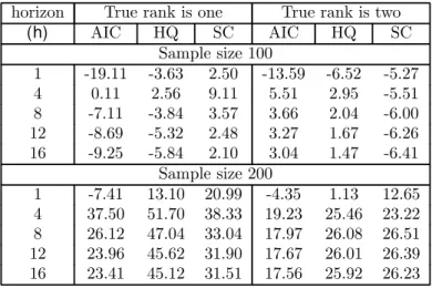
4.5. V ar iance-decom p osit ion r esult s
The percentage improvements of the estimated forecast-error variance decomposition coefficients are presented in Table 5. It is noticeable that there are virtually no signiÞcant gains at any horizon when the sample size is 100 observations. This is in sharp contrast with our benchmark case reported in Table 1, where there were gains of 20 to 74 percent for all reported horizons other than 1. This may
1 1Notice that this information is obtained by comparing the forecasting performance across di
be due to the fact that the variance contributions are ratios of estimated parameters. Although the allowance for rank restrictions improves the parameter estimates in a direction that leads to better forecasts, these improvements lead to worse estimates of the variance ratios when samples are small. When the sample size is 200, the quality of variance-decompositions based on models chosen byIC(p, r) is far superior to that of models chosen byIC(p).
5. Em pir ical Exam ple
The empirical analysis of the three-variable system that generates our simulated DGPs is discussed in Issler and Vahid (2001). There, we obtained a percentage reduction of 30.3% for the one-step ahead |M SF E| using the reduced-rank model. Here, we investigate a larger VAR which can be potentially useful for business-cycle analysis.
The “pulse” of the US economy is monitored every month by observing ßuctuations in four “coincident” variables, which are: 1) Personal income less transfer payments; 2) Index of industrial production; 3) Number of employees on nonagricultural payrolls; and 4) Manufacturing and trade sales12. In this section, we build a time-series model to forecast these coincident variables. It is
well-known that other series lead the coincident series and therefore help in forecasting them. See, for example, Stock and Watson (1989) or Zellner and Hong (1989). We follow Zellner and Hong and use measures of growth in real money balances and in the real rate of return of stocks as two leading indicator variables13. Since the coincident variables are not cointegrated (see Stock and Watson 1989), this constitutes a six-variable VAR for all of these log-differenced series, although our primary focus will be in forecasting the log-differences of the four coincident series alone14.
To make the empirical example conformable to our simulation study, we use monthly data from 1980:01 to 2000:07, a total of 247 observations. We develop our models on the basis of the Þrst 199 observations, leaving the last 48 observations for out-of-sample forecast evaluation. To be consistent with our simulation results, we select models using the Hannan-Quinn criterion. The full-rank version of theHQcriterion selects one lag for the six variable VAR. However, if we use the lag-rank version of HQ, the selected lag order is two and the selected rank is three. Therefore, we compare the performance of a full-rank VAR(1) with that of a reduced-rank VAR(2) in forecasting the four coincident variables. The estimated models are used to generate 48, 24, 16, and 12 non-overlapping one, two, three, and four-step ahead forecasts respectively, with results reported in Table 6. The out-of-sample forecasting results conform to those in our simulation study. For all
1 2The mnemonics for these variables in the DRI database are GMYXPQ, IP, LPNAG and MTQ respectively.
1 3
We use M2 deßated by producer price index as a measure of real balances (FM2/PWFSA in DRI) and S&P500 index deßated by the same price index (FSPCOM/PWFSA in DRI) in computing stock returns.
1 4We obtain similar results qualitatively when we consider forecasts of all six variables together. But forecasting
four short-run horizons, the reduced-rank model outperforms the full-rank model, with the largest percentage improvement of 23.8% for the |M SF E|at horizon four. This is a sizable improvement in forecasting accuracy.
It is informative to compare the univariate processes for individual variables implied by the estimated full rank VAR(1) model with those implied by the estimated rank 3 VAR(2) model. A full-rank 6 variable VAR(1) implies univariateARM A(6, q)processes for each of the variables, where
q is less than or equal to 5 and the autoregressive polynomials for all variables are identical. A rank 3 VAR(2) model implies univariateARM A(6, q) processes for individual variables, where q is less than or equal to 6 and autoregressive polynomials for all variables are identical15. All 6 roots of the implied autoregressive polynomial of the estimated full rank VAR(1) model turned out to be real, whereas there was a pair of complex conjugate roots among the 6 roots implied by the estimated rank 3 VAR(2) model. Because complex roots give rise to oscillatory components, and coincident and leading indicators are supposed to measure the cyclical oscillations in the economy, this gives further evidence in favor of the estimated reduced rank VAR(2) model.
Our conclusion from the empirical example is that if econometricians are interested in coincident and leading indicators, they should consider reduced-rank models at the model selection stage.
6. Conclusion
This paper argues that in multivariate macroeconometric modelling, the stylized fact that “macro-economic aggregates move together over the business cycle” should be taken seriously. Time series macro-econometric models provide useful forecasts for short horizons (1 to 8 periods). It is for these horizons that our Monte-Carlo study shows substantial gains in forecast accuracy if reduced-rank structures are allowed for. These gains are higher if the uncertainty about the lag length is assumed away, but they are still non-trivial in the more realistic case in which lag length and rank are chosen simultaneously.
The results of our Monte-Carlo analysis of model selection criteria that simultaneously select lag length and rank order can be summarized as follows. The tendency of AI C to choose overpa-rameterized models is worsened (particularly in small samples) when simultaneously choosing the rank and the lag length. Hence, we conclude thatAI C should not be used for this purpose in small samples. On the other hand, the tendency ofHQ and SC criteria to choose an underparameterized model is somewhat remedied when they are allowed to pick the rank and lag-length simultaneously. The SC criterion, however, still selects severely underparameterized models.
Contrary to previous literature that compares forecasts of VAR models selected by alternative model selection criteria, weÞnd no support for the claim that SC leads to models that produce the
1 5
best forecasts. We attribute this previous Þnding to the simple Monte Carlo design with short lag structures, that previous researchers have used. Indeed, in our simulations, the models selected by the Schwarz criterion produced worse forecasts than models chosen by the other two criteria. This was particularly evident in our simulations for the six-dimensional system16. Therefore, we conclude thatSC should not be used for model selection in high dimensional time series models, regardless of whether a reduced-rank structure is allowed for or not. Instead, we recommend the Hannan-Quinn criterion, which generally leads to models with the best forecast performance, especially when it is used for simultaneously choosing lag length and rank order.
Our analysis shows that there is a tension between efficiently estimating the mean parameters while allowing for reduced-rank structures, and efficiently estimating variance parameters. For samples of 100 observations we Þnd no gains from reduced rank structures in estimating variance decomposition coefficients. This result is reversed for larger samples of 200 observations. For the latter, there are non-trivial beneÞts in considering reduced-rank models in the estimation of variance contributions. Even though we have used all possible orderings of variables in performing our variance decompositions, we qualify ourÞndings in that the accuracy of the latter may not be invariant to the method of orthogonalizing the errors.
Finally, it should be stressed that the message of this paper is that short-run restrictions are likely to be more important than cointegrating restrictions, for forecasting at the business-cycle horizons. Here, we have only considered common-cycle restrictions because of their important macroeconomic implications. We leave the investigation of possible gains resulting form other restrictions, such as block exogeneity restrictions, codependence and other types of rank restrictions, for future research.
R efer ences
Ahn, S.K. and G.C. Reinsel (1988), “Nested reduced-rank autoregressive models for multiple time series”,Journal of the American Statistical Association, 83, 849-856.
Beveridge, S. and C.R. Nelson (1981), “A New Approach to Decomposition of Economic Time Se-ries into a Permanent and Transitory Components with Particular Attention to Measurement of the “Business Cycle”,Journal of Monetary Economics, vol. 7, pp. 151-174.
Carlino, G. and K. Sill (1998), “Common trends and common cycles in regional per-capita in-comes”, Working Paper, Federal Reserve Bank of Philadelphia.
Clements, M.P. and D.F. Hendry (1993), “On the limitations of comparing mean squared forecast errors,”Journal of Forecasting, 12, 617-637 (with discussions).
1 6The results for the six-dimensional system are not reported here to save space. They are reported in the working
Clements, M.P. and D.F. Hendry (1995), “Forecasting in cointegrated systems”, Journal of Ap-plied Econometrics, 10, 127-146.
Engle, R.F. and C.W.J. Granger (1987), “Cointegration and error correction: Representation, estimation and testing”,Econometrica, 55, 251-276.
Engle, R.F. and J.V. Issler (1995), “Estimating common sectoral cycles”, Journal of Monetary Economics, 35, 83-113.
Engle, R.F. and S. Yoo (1987), “Forecasting and testing in cointegrated systems”, Journal of Econometrics, 35, 143-159.
Granger, C.W.J., M.L. King and H. White (1995), “Comments on testing economic theories and the use of model selection criteria”,Journal of Econometrics, 67, 173-187.
Hamilton, J.D. (1994), T ime Series Analysis, Princeton University Press.
Issler, J.V. and F. Vahid (2001), “Common cycles and the importance of transitory shocks to macroeconomic aggregates,” forthcoming in theJournal of Monetary Economics.
Issler, J.V. and P.C. Ferreira (1998), “Time-Series properties and empirical evidence of growth and infrastructure,” T he Brazilian Review of Econometrics, vol. 18(1), pp. 31-71.
King, R., C.I. Plosser, J.H. Stock and M.W. Watson (1991), “Stochastic Trends and Economic Fluctuations”,American Economic Review, 81, 819-840.
King, R.G., C.I. Plosser and S. Rebelo (1988), “Production, Growth and Business Cycles. II. New Directions,” Journal of Monetary Economics, vol. 21, pp. 309-341.
Lin, J.L. and R.S. Tsay (1996), “Cointegration constraints and forecasting: An empirical exami-nation”, Journal of Applied Econometrics, 11, 519-538.
Lucas, R.E. (1977), “Understanding business cycles”,Carnegie-Rochester Series on Public Policy, 5, 7-29, also reprinted in Lucas, R. E. (Ed)Models of Business Cycle, 1977.
Lütkepohl, H. (1993), I ntroduction to Multiple T ime Series Analysis, Second Edition, Springer-Verlag.
Lütkepohl, H. (1985), “Comparison of criteria for estimating the order of a vector autoregressive process”, Journal of T ime Series Analysis, 6, 35-52.
Reinsel, G.C. (1993), Elements of Multivariate T ime Series Analysis, Springer-Verlag.
Stock, J.H. and M.W. Watson (1988), “Testing for common trends”, Journal of the American Statistical Association, 83, 1097-1107.
Stock, J. and Watson, M.(1989) “New Indexes of Leading and Coincident Economic Indicators”,
NBER Macroeconomics Annual, 351-95.
Tiao, G.C. and R.S. Tsay (1989), “Model speciÞcation in multivariate time series (with discus-sion)”, Journal of the Royal Statistical Society, Series B, 51, 157-213.
Tso, M.K-S. (1981), “Reduced rank regression and Canonical analysis” Journal of the Royal Statistical Society, Series B, 43, 183-189.
Vahid, F. (1999), “A property of the companion matrix of a reduced rank VAR”, Econometric T heory, 15, 787-788.
Vahid, F. and R.F. Engle (1993), “Common trends and common cycles”, Journal of Applied Econometrics, 8, 341-360.
Vahid, F. and Issler, J.V.(1999), “The Importance of Common-Cyclical Features in VAR Analysis: A Monte-Carlo Study,” Working Paper # 352, Graduate School of Economics, Getulio Vargas Foundation. Downloadable from www.fgv.br/epge/home/publi/Ensaios/ensaio_consulta.cfm.
Velu, R.P., G.C. Reinsel and D.W. Wickern (1986), “Reduced rank models for multiple time series”,Biometrika, 73, 105-118.
A pp endix
A . Syst em R
2and signal-t o-noise r at io
In a multiple regression with stochastic regressors and i.i.d. errors, y = Xβ +ε, the limiting signal-to-noise ratio (snr) can be deÞned as:
snr= β
0lim
T→∞E X
0X
T β
σ2
ε
, (A.1)
where E(εε0) = σ2
ε·I, and the proportion of the variation of dependent variable explained by the model, i.e. the population R2, is:
R2= β
0lim
T→∞E X
0X
T β
σ2
ε+β 0lim
T→∞E X
0X
T β
= snr (1+snr).
Since the asymptotic variance of √T β−β isAV AR(β) =σ2ε limT→∞E X 0X T
−1
, we can write (A.1) as:
snr=β0 AV AR(β) −1β. (A.2)
Consider now aV AR(p):
yt=A1yt−1+· · ·+Apyt−p+εt. (A.3) The analogous measure of snrfor it is:
snr=β0 Σ⊗Ω−1 β (A.4)
whereβ =vec(A),A= A1 . . . Ap ,E εtε0t−j =Ω, and:
Σ=
Γ0 Γ1 · · · Γp−1
Γ01 Γ0 · · · Γp−2
· · · · Γ0
p−1 Γ0p−2 · · · Γ0
,
where Γj = E ytyt0−j . Notice that Σ is completely determined by (A,Ω) via the Yule-Walker equations17. After some algebra, it can be shown that (A.4) is equal to:
snr=β0 Σ⊗Ω−1 β=trace Γ0Ω−1 −n.
Using this last result, one can then deÞne the systemR2to be:
R2= trace Γ0Ω
−1
−n 1+trace(Γ0Ω−1)−n
.
1 7
Table 1: Percentage improvement in different forecast accuracy measures and in the MSE of forecast-error variance decompositions when the true rank restrictions are imposed
horizon True rank is one True rank is two
(h) GFESM |MSFE| TMSFE Var. Dec. GFESM |MSFE| TMSFE Var. Dec.
Sample size 100
1 22.22 22.22 1.97 -10.68 12.08 12.08 0.98 -7.67
4 60.41 8.66 1.72 73.93 34.56 5.02 0.96 20.69
8 70.54 1.70 1.39 54.03 42.57 1.32 0.77 21.38
12 72.34 0.46 1.03 52.41 44.66 0.45 0.59 21.76
16 72.86 0.21 0.81 52.06 45.26 0.25 0.47 21.88
Sample size 200
1 11.22 11.22 1.14 -6.00 6.55 6.55 0.60 -3.55
4 29.53 3.80 0.88 94.05 17.80 2.32 0.52 27.19
8 32.97 0.52 0.64 66.65 20.72 0.46 0.37 27.01
12 33.37 0.11 0.45 63.96 21.19 0.07 0.27 27.19
Table 2.a: Frequency of lag (p) and lag-rank (p, r ) choice by different criteria when the true models are (4, 1)
Selected lag 1 2 3 4 5 6 7 8
Selected rank 1 2 3 1 2 3 1 2 3 1T 2 3 1 2 3 1 2 3 1 2 3 1 2 3
Number of observations=100
AI C (p) − − 57.0 − − 13.1 − − 12.6 − − 14.0 − − 2.0 − − 0.7 − − 0.3 − − 0.3
AI C (p, r ) 10.8 2.5 0.4 7.4 2.0 0.1 14.4 2.4 0.1 32.7 3.4 * 8.3 1.1 * 5.0 0.6 * 3.8 0.4 * 4.0 0.5 *
H Q (p) − − 92.9 − − 4.7 − − 1.7 − − 0.7 − − * − − * − − 0 − − 0
H Q (p, r ) 39.2 1.9 0.2 13.3 0.3 * 17.0 0.1 * 24.3 0.1 * 2.4 * 0 0.7 * 0 0.3 0 0 0.1 0 0
SC (p) − − 99.6 − − 0.4 − − * − − * − − 0 − − 0 − − 0 − − 0
SC (p, r ) 73.8 0.4 * 10.7 * 0 8.4 0 0 6.6 0 0 0.1 0 0 * 0 0 0 0 0 0 0 0
Number of observations=200
AI C (p) − − 25.9 − − 10.7 − − 20.0 − − 40.0 − − 2.7 − − 0.5 − − 0.2 − − *
AI C (p, r ) 2.2 0.7 0.1 3.3 0.8 * 12.1 1.8 * 56.4 4.1 0.1 9.1 0.8 * 4.1 0.3 0 2.3 0.1 0 1.6 0.1 0
H Q (p) − − 80.1 − − 7.8 − − 7.2 − − 4.9 − − * − − 0 − − 0 − − 0
H Q (p, r ) 16.1 0.6 0.1 8.9 0.1 * 20.7 0.1 0 51.3 * 0 1.9 0 0 0.2 0 0 * 0 0 * 0 0
SC (p) − − 98.6 − − 1.0 − − 0.3 − − 0.1 − − 0 − − 0 − − 0 − − 0
SC (p, r ) 49.4 0.1 * 11.1 * 0 17.1 0 0 22.3 0 0 0.1 0 0 * 0 0 0 0 0 0 0 0
Table 2.b: Frequency of lag (p) and lag-rank(p, r ) choice by different criteria when the true models are(4, 2)
Selected lag 1 2 3 4 5 6 7 8
Selected rank 1 2 3 1 2 3 1 2 3 1 2T 3 1 2 3 1 2 3 1 2 3 1 2 3
Number of observations=100
AI C (p) − − 19.9 − − 10.2 − − 21.3 − − 41.3 − − 4.6 − − 1.5 − − 0.7 − − 0.5
AI C (p, r ) 1.1 4.9 1.0 1.0 4.7 0.6 2.5 15.5 1.2 4.3 43.7 1.8 1.2 7.0 0.3 0.8 3.1 0.1 0.7 1.8 * 0.9 1.6 *
H Q (p) − − 64.1 − − 13.1 − − 12.7 − − 9.9 − − 0.1 − − * − − 0 − − 0
H Q (p, r ) 8.6 19.6 1.9 5.0 8.1 0.2 8.1 14.8 0.1 10.5 20.8 * 1.1 0.6 0 0.4 0.1 0 0.1 * 0 0.1 * 0
SC (p) − − 93.2 − − 5.1 − − 1.5 − − 0.2 − − 0 − − 0 − − 0 − − 0
SC (p, r ) 30.3 30.6 1.2 9.5 4.8 * 9.4 4.3 * 7.9 1.9 0 0.2 * 0 * 0 0 * 0 0 0 0 0
Number of observations=200
AI C (p) − − 3.3 − − 2.7 − − 16.3 − − 72.2 − − 4.3 − − 0.8 − − 0.2 − − 0.1
AI C (p, r ) 0.1 0.6 0.2 0.1 0.9 0.1 0.3 10.2 0.7 0.9 72.3 2.5 0.2 7.1 0.2 0.1 2.0 * 0.1 0.8 * 0.1 0.4 *
H Q (p) − − 27.9 − − 9.6 − − 23.3 − − 39.2 − − * − − 0 − − 0 − − 0
H Q (p, r ) 1.3 7.5 0.6 0.9 4.7 * 3.4 20.0 * 4.7 56.2 * 0.2 0.4 0 * * 0 * 0 0 * 0 0
SC (p) − − 74.4 − − 10.4 − − 10.3 − − 5.0 − − 0 − − 0 − − 0 − − 0
SC (p, r ) 9.2 26.9 0.7 4.3 6.8 * 8.2 15.1 0 9.1 19.8 0 * * 0 * 0 0 0 0 0 0 0 0
Table 3a: Percentage improvement in different measures of accuracy in forecasts generated by the possibly reduced rank VAR over the full rank VAR chosen by the same model selection criterion when the true models are trivariate (4,1)
horizon AIC HQ SC
(h) GFESM |MSFE| TMSFE GFESM |MSFE| TMSFE GFESM |MSFE| TMSFE
Sample size 100
1 6.6 6.6 0.0w 6.8 6.8 2.8b 5.3 5.3 1.6
4 10.8 2.3 1.1 16.1 6.1 4.8b 10.9 4.1 3.0w
8 4.0 -1.0 0.0 15.1 -0.3 2.7b 11.0 -0.1 1.7w
12 2.0 -0.6 -0.2w 14.2 -0.2 1.7b 10.7 -0.1 1.1
16 1.0 -0.3 -0.2w 13.7 -0.2 1.2b 10.5 -0.1 0.8
Sample size 200
1 9.1 9.1 2.0b 11.0 11.0 6.7 8.3 8.3 5.3w
4 22.2 3.2 2.0b 30.8 8.2 7.7 22.5 7.1 6.8w
8 22.1 0.1 1.0b 31.8 0.5 4.4 23.4 0.4 3.9w
12 22.1 0.0 0.7 31.7 0.0 2.8b 23.4 0.0 2.6w
16 22.0 0.0 0.5 31.7 0.0 2.1b 23.3 0.0 1.9w
Table 3b: Percentage improvement in different measures of accuracy in forecasts generated by the possibly reduced rank VAR over the full rank VAR chosen by the same model selection criterion when the true models are trivariate (4,2)
horizon AIC HQ SC
(h) GFESM |MSFE| TMSFE GFESM |MSFE| TMSFE GFESM |MSFE| TMSFE
Sample size 100
1 7.6 7.6 0.1 5.9 5.9 2.2b 1.6 1.6 1.4w
4 19.2 2.9 0.5 19.2 6.1 3.9b 10.1 6.1 4.3w
8 20.4 0.1 0.1 19.7 -0.0 2.2b 10.0 -0.0 2.5w
12 20.5 0.0 0.0 19.6 -0.1 1.4b 9.4 -0.0 1.6w
16 20.5 0.1 0.0 19.4 -0.1 1.0b 9.1 -0.1 1.2w
Sample size 200
1 5.9 5.9 0.7b 6.8 6.8 2.3 8.8 8.8 5.4w
4 15.3 2.0 0.5b 20.5 4.3 2.6 28.7 8.9 6.5w
8 17.1 0.2 0.3b 21.7 0.3 1.5 31.1 0.6 3.7w
12 17.3 0.0 0.2b 21.8 0.0 1.0 31.3 0.1 2.5w
16 17.3 0.0 0.1b 21.7 0.0 1.0 31.2 -0.0 1.8w
Table 4a: Percentage improvement in different measures of accuracy in forecasts generated by the possibly reduced-rank VAR model chosen by sequential rank testing
over that of the full rank VAR when the true models are trivariate (4,1)
horizon AIC HQ SC
(h) GFESM |MSFE| TMSFE GFESM |MSFE| TMSFE GFESM |MSFE| TMSFE
Sample size 100
1 8.4 8.4 0.7 3.7 3.7 0.3 3.1 3.1 0.2
4 18.3 2.1 0.5 4.8 0.1 0.1 3.4 -0.0 0.0
8 21.4 0.6 0.4 5.1 0.0 0.0 3.5 -0.0 0.0
12 22.2 0.2 0.3 5.2 0.0 0.0 3.5 -0.0 0.0
16 22.5 0.1 0.3 5.2 0.0 0.0 3.5 -0.0 0.0
Sample size 200
1 7.1 7.1 0.7 2.7 2.7 0.2 1.8 1.8 0.1
4 17.4 1.9 0.5 4.7 0.2 0.1 1.9 -0.0 0.0
8 19.5 0.3 0.4 5.1 0.1 0.1 2.0 -0.0 0.0
12 19.8 0.1 0.3 5.1 0.0 0.1 2.0 -0.0 0.0
16 20.0 0.1 0.2 5.2 0.0 0.0 2.0 0.0 0.0
Table 4b: Percentage improvement in different measures of accuracy in forecasts generated by the possibly reduced-rank VAR model chosen by sequential rank testing
over that of the full rank VAR when the true models are trivariate (4,2)
horizon AIC HQ SC
(h) GFESM |MSFE| TMSFE GFESM |MSFE| TMSFE GFESM |MSFE| TMSFE
Sample size 100
1 7.7 7.7 0.4 2.9 2.9 0.0 0.2 0.2 -0.3
4 21.5 3.0 0.5 7.6 1.0 0.2 0.7 0.2 0.0
8 27.3 1.0 0.5 9.2 0.2 0.2 0.9 -0.0 0.0
12 28.9 0.4 0.4 9.7 0.1 0.1 0.9 0.0 0.0
16 29.6 0.2 0.3 10.0 0.1 0.1 0.9 0.0 0.0
Sample size 200
1 5.5 5.5 0.5 3.9 3.9 0.3 1.3 1.3 0.1
4 14.6 1.9 0.4 9.8 1.2 0.3 2.9 0.3 0.1
8 17.1 0.4 0.3 11.4 0.2 0.2 3.3 0.1 0.1
12 17.6 0.1 0.2 11.7 0.1 0.1 3.4 0.0 0.0
16 17.7 0.1 0.2 11.7 0.1 0.1 3.4 0.0 0.0
Table 5: Percentage improvement in MSE of forecast-error variance decomposition generated by the possibly reduced rank VAR over
the full rank VAR chosen by the same model selection criterion
horizon True rank is one True rank is two
(h) AIC HQ SC AIC HQ SC
Sample size 100
1 -19.11 -3.63 2.50 -13.59 -6.52 -5.27
4 0.11 2.56 9.11 5.51 2.95 -5.51
8 -7.11 -3.84 3.57 3.66 2.04 -6.00
12 -8.69 -5.32 2.48 3.27 1.67 -6.26
16 -9.25 -5.84 2.10 3.04 1.47 -6.41
Sample size 200
1 -7.41 13.10 20.99 -4.35 1.13 12.65
4 37.50 51.70 38.33 19.23 25.46 23.22
8 26.12 47.04 33.04 17.97 26.08 26.51
12 23.96 45.62 31.90 17.67 26.01 26.39
16 23.41 45.12 31.51 17.56 25.92 26.23
Table 6: Forecasting performance of alternative models of coincident variables
Model Full-rankV AR (1) Rank 3V AR (2)
Horizon |MSFE| TMSFE |MSFE| TMSFE
1 month ahead 0.3437×10⁻⁴ 0.6241 0.3107×10⁻⁴ 0.5647 2 months ahead 0.1374×10⁻⁴ 0.5932 0.1156×10⁻⁴ 0.5442 3 months ahead 0.0683×10⁻⁴ 0.5534 0.0651×10⁻⁴ 0.5166 4 months ahead 0.0868×10⁻⁴ 0.5643 0.0701×10⁻⁴ 0.4916