❊♥s❛✐♦s ❊❝♦♥ô♠✐❝♦s
❊s❝♦❧❛ ❞❡
Pós✲●r❛❞✉❛çã♦
❡♠ ❊❝♦♥♦♠✐❛
❞❛ ❋✉♥❞❛çã♦
●❡t✉❧✐♦ ❱❛r❣❛s
◆◦ ✹✹✶ ■❙❙◆ ✵✶✵✹✲✽✾✶✵
❚❡st✐♥❣ Pr♦❞✉❝t✐♦♥ ❋✉♥❝t✐♦♥s ❯s❡❞ ✐♥ ❊♠✲
♣✐r✐❝❛❧ ●r♦✇t❤ ❙t✉❞✐❡s
P❡❞r♦ ❈❛✈❛❧❝❛♥t✐ ●♦♠❡s ❋❡rr❡✐r❛✱ ❏♦ã♦ ❱✐❝t♦r ■ss❧❡r✱ ❙❛♠✉❡❧ ❞❡ ❆❜r❡✉ P❡ss♦❛
❖s ❛rt✐❣♦s ♣✉❜❧✐❝❛❞♦s sã♦ ❞❡ ✐♥t❡✐r❛ r❡s♣♦♥s❛❜✐❧✐❞❛❞❡ ❞❡ s❡✉s ❛✉t♦r❡s✳ ❆s
♦♣✐♥✐õ❡s ♥❡❧❡s ❡♠✐t✐❞❛s ♥ã♦ ❡①♣r✐♠❡♠✱ ♥❡❝❡ss❛r✐❛♠❡♥t❡✱ ♦ ♣♦♥t♦ ❞❡ ✈✐st❛ ❞❛
❋✉♥❞❛çã♦ ●❡t✉❧✐♦ ❱❛r❣❛s✳
❊❙❈❖▲❆ ❉❊ PÓ❙✲●❘❆❉❯❆➬➹❖ ❊▼ ❊❈❖◆❖▼■❆ ❉✐r❡t♦r ●❡r❛❧✿ ❘❡♥❛t♦ ❋r❛❣❡❧❧✐ ❈❛r❞♦s♦
❉✐r❡t♦r ❞❡ ❊♥s✐♥♦✿ ▲✉✐s ❍❡♥r✐q✉❡ ❇❡rt♦❧✐♥♦ ❇r❛✐❞♦ ❉✐r❡t♦r ❞❡ P❡sq✉✐s❛✿ ❏♦ã♦ ❱✐❝t♦r ■ss❧❡r
❉✐r❡t♦r ❞❡ P✉❜❧✐❝❛çõ❡s ❈✐❡♥tí✜❝❛s✿ ❘✐❝❛r❞♦ ❞❡ ❖❧✐✈❡✐r❛ ❈❛✈❛❧❝❛♥t✐
❈❛✈❛❧❝❛♥t✐ ●♦♠❡s ❋❡rr❡✐r❛✱ P❡❞r♦
❚❡st✐♥❣ Pr♦❞✉❝t✐♦♥ ❋✉♥❝t✐♦♥s ❯s❡❞ ✐♥ ❊♠♣✐r✐❝❛❧ ●r♦✇t❤ ❙t✉❞✐❡s✴ P❡❞r♦ ❈❛✈❛❧❝❛♥t✐ ●♦♠❡s ❋❡rr❡✐r❛✱ ❏♦ã♦ ❱✐❝t♦r ■ss❧❡r✱ ❙❛♠✉❡❧ ❞❡ ❆❜r❡✉ P❡ss♦❛ ✕ ❘✐♦ ❞❡ ❏❛♥❡✐r♦ ✿ ❋●❱✱❊P●❊✱ ✷✵✶✵
✭❊♥s❛✐♦s ❊❝♦♥ô♠✐❝♦s❀ ✹✹✶✮ ■♥❝❧✉✐ ❜✐❜❧✐♦❣r❛❢✐❛✳
Testing Production Functions Used in
Empirical Growth Studies
∗
Pedro Cavalcanti Ferreira
†João Victor Issler
Samuel de Abreu Pessôa
Graduate School of Economics - EPGE
Getulio Vargas Foundation
March 2002
Abstract
We estimate and test two alternative functional forms represent-ing the aggregate production function for a panel of countries: the extended neoclassical growth model, and a mincerian formulation of schooling-returns to skills. Estimation is performed using instrumental-variable techniques, and both functional forms are confronted using a Box-Cox test, since human capital inputs enter in levels in the min-cerian speciÞcation and in logs in the extended neoclassical growth model. Our evidence rejects the extended neoclassical growth model in favor of the mincerian speciÞcation, with an estimated capital share of about 42%, a marginal return to education of about 7.5% per year, and an estimated productivity growth of about 1.4% per year. Dif-ferences in productivity cannot be disregarded as an explanation of
∗We gratefully acknowledge the comments and suggestions of an anonymous referee, Costas Azariadis, Gary Hansen, Marcos B. Lisboa, Carlos Martins-Filho, Naércio Menezes, Alberto Trejos, Farshid Vahid, Martin Uribe, and several seminar participants around the world. All remaining errors are ours. Rafael Martins de Souza and José Diogo Barbosa provided excellent research assistance. The authors also acknowledge theÞnancial support of CNPq-Brazil and PRONEX.
why output per worker varies so much across countries: a variance decomposition exercise shows that productivity alone explains 54% of the variation in output per worker across countries.
1
Introduction
In this paper we estimate and test two alternative functional forms, which have been used in the growth literature, representing the aggregate produc-tion funcproduc-tion for a panel of countries. TheÞrst model we consider has a long tradition in the growth literature — the extended neoclassical growth model — and was proposed by Mankiw, Romer and Weil(1992), among others. The second is a mincerian formulation of schooling-returns to skills, traditionally used in the labor-economics literature, e.g., Mincer(1974) and Wills(1986), but recently incorporated into the growth literature as well, e.g., Bils and Klenow(1996), and Hall and Jones(1999). In the latter case, schooling enters exponentially in the production function, while in the former it does not, paralleling the way physical capital is modelled.
Estimation is performed using instrumental-variable techniques, suitable for panels, after a careful search for appropriate instruments. After estima-tion, we ask which of these two functional forms best Þts the data, using a variety of speciÞcation tests, including tests of the validity of instruments, tests ofÞxed vs. random effects, and of the restriction that productivity is the same across countries. Finally, both functional forms are confronted using a Box-Cox test. The data are extracted from Summers and Heston(1991, mark 5.6) and Barro and Lee(1996), and include 95 countries in different stages of economic development, with observations ranging from 1960 to 1985.
im-portant factor in explaining the differences of output per worker across coun-tries; see, for example, Hall and Jones(1999), Prescott(1998), and Klenow and Rodriguez-Clare(1997).
The conclusions in these articles are somewhat inßuenced by their method-ological choices, particularly by the choice of the functional form of the aggre-gate production function and by the choice of the estimation method and/or by the parameter calibration employed. A simple variance decomposition along the lines of Hall and Jones and Klenow and Rodriguez-Clare shows that if the capital share is calibrated as in Chari, Kehoe and McGrattan (2/3), factors of production alone explain 82% of the variance of output per worker. On the other hand, if the capital share is calibrated as in Hall and Jones (1/3), productivity alone explains 61% of output-per-worker variance, an opposite result. Hence, before looking at speciÞc growth accounting ex-ercises, one must be conÞdent on the validity of the assumptions behind it.
Our evidence rejects the extended neoclassical growth model in favor of the mincerian speciÞcation, with an estimated capital share of about 42%, a marginal return to education of about 7.5% per year, and an estimated productivity growth of about 1.4% per year. Productivity estimates vary considerably across countries, and testing whether productivity is the same for all countries strongly rejects this hypothesis. Moreover, differences in productivity cannot be disregarded as an explanation of why output per worker varies so much across countries: a variance decomposition exercise shows that productivity alone explains 54% of the variation in output per worker across countries, a result along the lines of Hall and Jones and of Klenow and Rodriguez-Clare.
Bils and Klenow, Hall and Jones, and Klenow and Rodriguez-Clare make the case for the mincerian form based on microeconomic evidence. The present study conÞrms the appropriateness of this approach from a macro-economic perspective. It is also comforting to note that our estimate of the marginal return to education is consistent with those obtained in micro studies. These results increase our conÞdence that the mincerian speciÞ ca-tion should be used in future studies and also the conÞdence with which we regard the growth-accounting results based on it.
Section 5 concludes.
2
Model Speci
Þ
cation
The Þrst production function considered here is the so-called “extended neo-classical growth model,” which uses human capital as an additional explana-tion for output, jointly with physical capital and raw labor. Start with the following homogenous-of-degree-one production function:
Yit =AitF (Kit, Hit, Litexp (g·t)), (1)
where Yit, Kit, Hit, Lit, and Ait are respectively output, physical capital,
human capital, raw labor inputs, and productivity for country i in periodt, where i= 1,· · · , N, andt = 1,· · · , T. It is assumed that there is exogenous technological progress at rate g, which is the same across countries. The production function in per-worker terms can be written as:
Yit
Lit
=yit =AitF (kit, hit,exp (g·t)). (2)
Assuming Cobb-Douglas technology (or using aÞrst-order log-linear approx-imation of the above function) gives:
lnyit = lnAit+αlnkit+βlnhit+γg·t+εit, (3)
where εit is the inherited measurement error for country i in period t.
Im-posing homogeneity explicitly (i.e., γ = (1−α−β)), we obtain the following:
lnyit= lnAi+αlnkit+βlnhit+ (1−α−β)g·t+ηit, (4)
where in (4) Ait is decomposed into a time-invariant component Ai and a
component that varies across i andt - νit, such thatηit =νit+εit.
The second speciÞcation differs from the above in the way human cap-ital is modelled. It uses a mincerian (e.g., Mincer(1974) and Wills(1986)) formulation of schooling returns to skills to model human capital. There is only one type of labor in the economy, which has skill levelλ, determined by educational attainment. It is assumed that the skill level of a worker with
h years of schooling is exp (φh) greater than that of a worker with no edu-cation at all, leading to the following homogenous-of-degree-one production function:
The parameter φ in λit = exp (φhit) gives the skill return of one extra
year of education, i.e., φ can be interpreted as a measure of the percentage increase in income of an additional year of schooling. In per-worker terms, the equation above reduces to:
Yit
Lit
=yit=AitF(kit,λitexp (g·t)). (6)
Again, with Cobb-Douglas technology (or with a Þrst order log-linear approximation of the production function) we obtain:
lnyit= lnAit+αlnkit+βln (λitexp (g·t)) +εit, (7)
whereεitis the inherited measurement error for countryiin periodt. Finally,
using λit = exp (φhit) and imposing homogeneity explicitly (i.e., β= 1−α),
we obtain:
lnyit= lnAi+αlnkit+ (1−α)(φhit+g·t) +ηit, (8)
where, again, in (8) Ait is decomposed into a time-invariant component Ai
and a component that varies across i andt - νit, such that ηit =νit+εit.
Econometrically, the basic difference between equations (4) and (8) is whether human capital enters the (log of the) production function in levels or in logs. If human capital enters in logs — (4), there is aÞxed human-capital elasticity in production for all countries. If it enters in levels — (8), human-capital elasticity in production will change across countries (and across time as well).
3
Econometric Estimation, Testing, and
Re-sults
3.1
Estimation and Testing
When choosing between these two types of speciÞcations in regression mod-els, it is customary to resort to the so called “Box and Cox(1964) transfor-mation.” Consider the generic regression equation, using the Box and Cox transformation for the regressor:
yt=
µ
xθ
t −1
θ ¶
β+εt. (9)
Notice that:
lim θ→0
µ
xθ
t −1
θ ¶
= ln (xt), and (10)
lim θ→1
µ
xθ
t −1
θ ¶
= xt−1, (11)
where it is clear that for a logarithmic transformation to be valid we must have θ = 0, and for the series xt to enter the regression in levels we must
have θ= 1.
These two hypotheses can be tested by means of a Wald test, using a Box-Cox transformation for the human-capital measure in the production function. This is exactly how we proceed here. However, since we impose constant returns to scale in both production functions (4) and (8), there is not a general regression model which nests them. Therefore, we proceed in testing these two functional forms before imposing constant returns to scale constraints in production. We next discuss other modelling choices made here.
Each one of the sets of equations in (4) and (8) constitutes a structural system of equations for a set of countries i = 1,2,· · ·N and a set of time periods t = 1,2,· · ·T. As is usual with such a panel, panel-data techniques can be employed to estimate the structural parameters lnAi,α,β, g, andφ.
If one disregards the panel-data structure in either (4) or (8), exploiting only the cross-sectional dimension of the data set, one cannot estimate either the technological-progress trend coefficient g, or the country-speciÞc productiv-ity level lnAi. Trying to do so would inevitably exhaust all available degrees
of freedom. This is the main criticism of Islam(1995) of the estimation pro-cedure in Mankiw, Romer and Weil(1992). Because we do not want to rule out a priori that lnAi can be an important factor in explaining the
rather than imposing, we test the hypothesis that productivity varies across countries, which has not been done previously.
In considering the techniques to be employed in estimating either (4) or (8), the following have to be taken into account: (i) in general, lnkit, lnhit,
and hit are correlated with ηit. This occurs for several reasons. In a short
list, lnkit, lnhit, and hit are measured with error, generating an
error-in-variables problem in estimation. Second, there is a portion of ηit that comes from productivity, hence being correlated withlnkit,lnhit, and hit. Because
regressors and errors are correlated, if one hopes to get consistent estimates of structural parameters, a list of instrumental variables has to be obtained. These must be correlated with lnkit, lnhit, and hit, but not with ηit; (ii) a
choice must be made regarding how to model lnAi. There are two natural
candidates in the panel-data literature: modelling lnAi as a Þxed effect or
as a random effect.
Simultaneous-equation coefficients, such as the ones in either (4) or (8) above, can be consistently estimated by instrumental variable methods; see Hsiao(1986, pp. 115-127). Considering the structure of correlation among errors for different countries is aÞrst step in choosing the estimation method. A reasonable assumption about errors is that their variance is not identical across countries, maybe due to the fact that shocks to speciÞc countries are different. Errors for different countries should also have a non-zero contem-poraneous correlation, because of common international shocks that simul-taneously affect all countries. Exploiting this leads to efficiency gains in estimation, i.e., more precise parameter estimates.
In our case we have 26 years of data and 95 countries. If the estimate of
lnAi is to vary across countries as aÞxed effect, for example, is is not feasible
to fully exploit these efficiency gains, because the estimate of the variance-covariance matrix of the errors will be singular. Moreover, full information methods (such as full information maximum likelihood or 3SLS) also have problems of their own, in which mis-speciÞcation of one given equation in the system carries over to other system equations, leading to inconsistent estimates for the whole system. The larger the system, the higher the chance of mis-speciÞcation. For these reasons, we choose to estimate (4) and (8) in a limited information setting. However, heteroskedasticity of errors in different countries will be considered in estimation. This is done by weighting every equation in the system differently, using the reciprocals of the standard deviations of the country-speciÞc errors as weights.
instruments. We discuss here the case of the (log of) the capital stock, but a similar argument applies to the measures of human capital as well (lnhit
or hit). Consider Þrst lnkjt−1,i6=j, i.e., the lagged (log level of the) capital
stock of country j, as an instrument for lnkit1. Even if the capital stock is
measured with error, creating an error-in-variable problem, as long as the measurement errors are idiosyncratic in nature (country speciÞc), lnkjt−1
will not be correlated with ηit. A possible problem is that it may not be correlated with lnkit either. For example, there is no guarantee that the
lagged (log of the) capital stock of Fiji will be correlated with the current (log of the) capital stock of Romania. However, if we choose a group of countries
j satisfying some geographical (or cultural) criterion, we can increase the chance oflnkjt−1 andlnkit being correlated. In particular, we propose using
for each country i the following instrument forlnkit:
1 Ni
X
j∈{Ni}
lnkjt−1, (12)
where Ni represents the number of additional countries in the same
conti-nent that country i is in, and {Ni} represents the set of countries in that
continent that are not country i, i.e., (12) represents rest-of-the-continent average lagged (log of the) capital stock.
Lagged average rest-of-continent capital stock looks promising as an in-strument. Countries in the same continent usually trade more with each other than with countries outside that continent. They also tend to have similar macroeconomic policies. These factors contribute to deliver a non-zero correlation between N1i
P
j∈{Ni}lnkjt−1 and lnkit. On the other hand,
one can argue that some component of 1 Ni
P
j∈{Ni}lnkjt−1 may be correlated
withηit. Although this is always possible, there is a way that the orthogonal-ity between errors and instruments can be tested for over-identiÞed models; basic references are Sargan(1958) and Basmann(1960).
Testing orthogonality for a speciÞc over-identiÞed regression equation in a system requires Þrst using instrumental-variable residuals in running aux-iliary regressions, and second constructing a T ×R2 statistic with the
out-put of this auxiliary regression; see Davidson and MacKinnon(1993, Sec-tion 7.8). Although the procedure is suitable for testing “orthogonality” for
1We choose the lagged capital stock for country j to reduce further the chance of
single-equations in a system, it is a joint test of orthogonality and of cor-rect speciÞcation of the model. Hence, rejection of the null can be due to incorrect speciÞcation and not to lack of orthogonality. This requires avoid-ing imposavoid-ing any restrictions on panel-regression estimates when testavoid-ing for orthogonality.
Finally, whether we should use Þxed or random effects in modelling in-dividual productivity factors lnAi can be investigated by means of a
Haus-man(1978) test. Estimates using Þxed and random effects are compared by searching for departures of the latter from the former, which happens when the random component is correlated with regressors. A large difference is a sign of a non-zero correlation, which violates consistency for the parameters of the random effect model.
3.2
The Data
The panel data set used ranges from 1960 to 1985, and combines macroeco-nomic data for 95 countries in the mark 5.6 of the Summers and Heston (SH, from now on) data set with human-capital measures extracted from Barro and Lee(1996). Since the latter are only available at Þve-year intervals, we Þrst considered using a database with that frequency. However, this presents a problem, since production-function data will use non-contiguous observations and several years of data would be left unused. Alternatively, we decided to interpolate human-capital measures to Þt annual frequency. Although this induces measurement error in human capital, the problem is relatively small, since human capital changes with a highly predictable pattern and the esti-mation technique used allows for regressors that are measured with error2.
The time span was restricted from 1960 to 1985. Before the 1960’s, and after 1985, macroeconomic data is missing for several developing countries. Limiting the Þnal year to 1985 also has the advantage of including in our sample the previously socialist countries. Most of them made their transition into capitalism at the end of the 1980’s, making 1985 the last possible year to include in the sample.
The speciÞc series used are the following: yit is the ratio of real GDP
(at 1985 international prices) and the number of workers in the labor force, extracted from SH;kit is the physical capital series per worker. The physical 2To check the robustness of estimation results, we compared those using data with
capital series is constructed using real investment data from SH (at 1985 international prices); hit is Barro and Lee’s(1996) series of average years of
completed education of the labor force, interpolated (in levels) to Þt annual frequency.
The way the physical-capital series were constructed deserves comment. We started with the investment series and applied the Perpetual Inventory Method to get measures of capital. This method requires an initial capital level and a depreciation rate for physical capital. Since it is not obvious which is a reasonable depreciation rate to apply for all countries, we chose to use Þve different rates (3%, 6%, 9%, 12%, and 15%), checking whether the capital series were similar across depreciation rates. As for the initial capital stock, we followed Young(1995) and Hall and Jones(1999) and approximated it by K0 =I0/(gI+δ), whereK0 is the initial capital stock, I0 is the initial
investment expenditure, gI is the growth rate of investment, and δ is the
depreciation rate of the capital stock. Since gI is the (population) mean
growth rate of investment, the closest we can get to it is by computing sample long-term time averages. That is exactly how we proceed here3.
3.3
Model Estimation Results
Instrumental-variable estimates of the mincerian model (8), using a limited-information setting for a variety of depreciation rates for the capital stock, are presented in Table 1. It also includes several test results — Box-Cox, Haus-man, Sargan, etc. Instruments are country-speciÞc, comprisingN1i
P
j∈{Ni}lnkjt−1, 1
Ni
P
j∈{Ni}hjt−1, andt, and productivity (lnAi) is modelled as aÞxed-effect.
The latter is the result of a Hausman(1978) test for choosing how to model
lnAi (random versus Þxed effects); see the p-values for it in Table 1.
< include Table 1 here>
3Notice that Young(1995) uses the mean growth of investment in the ÞrstÞve years
of his sample as a proxy for gI. As argued in the text, it is preferable to use long-term time averages because 1/TPTt=1gIt converges in probability togI, and for large enough
T, these sample averages are close to gI. Moreover, for the period of time in question, had we adopted Young’s procedure, we would have biased our estimate of K0downward,
The reported estimates for α, φ, and g do not change much as we vary depreciation rates. For reasonable values ofδ(6%-12% interval), the estimate of α is about 0.41, of φabout 0.08, and of g about 0.014; all are statistically signiÞcant at the usual levels.
These numbers are close to what could be expecteda priori: several cali-brated studies use a capital elasticityα= 1/3(see Cooley and Prescott(1995)). Estimates in Gollin(1997) are also close to 0.40 for a variety of countries, and those in Islam(1995) are 0.52 for non-oil countries — smaller for intermedi-ate and OECD countries. As discussed above, φ can be interpreted as a measure of the percentage increase in income of an additional year of school-ing. Mincerian regressions usually Þnd bφ '10% (Mincer(1974)). Moreover, Psacharopolos(1994), who surveys schooling-return evidence using a large set of countries, Þnds an average of 6.8% for OECD countries and 10.1% for the world as a whole. It is therefore comforting to be able to reconcile our growth-regression results, using a macroeconomic model, with the micro-economic evidence found elsewhere on returns to schooling. Regarding the estimate ofg, an average growth rate of productivity of 1.4% a year is in line with the evidence on long-run growth presented by Maddison(1995).
Instrumental-variable estimates of the extended neoclassical growth model (4) are presented in Table 2. The same country-speciÞc instruments were used. Due to a Hausman-test result, productivity (lnAi) is modelled as a
Þxed effect. For reasonable depreciation rates (6%-12% interval), the esti-mate ofα is about 0.43, close to that in the mincerian case. The estimate of the growth rate of productivity g is about 1.9% a year, maybe closer to the conventional wisdom than the mincerian estimate. Human capital elasticity estimates bβ are relatively small: about 0.025 and, for some values of δ, not signiÞcantly different from zero; see Islam(1995) for a similar result.
< include Table 2 here>
The results in Table 2 are completely different from those obtained by Mankiw, Romer and Weil(1992), in which their estimated sum of the shares of capital and labor are much higher: ours are at most 0.45, while theirs is about 0.60. In order to reconcile these conßicting results we re-estimated the extended neoclassical model under the restriction that productivity is the same across countries, i.e., thatln (Ai) = ln (A), ∀i; see the discussion in
to 0.60, the second jumps from 0.02 to 0.11 — about Þve times higher, and their sum increases from about 0.45 to about 0.71. Hence, if productivity is restricted such that ln (Ai) = ln (A),∀i, estimates closer to Mankiw, Romer
and Weil’s are produced. We perform a Wald test for ln (Ai) = ln (A), ∀i.
Results of these tests for the mincerian and the extended neoclassical model are presented respectively in the last lines of Tables 1 and 2. Test results overwhelmingly reject these restrictions, showing that the Þxed-effect
speci-Þcation is appropriate, and that productivity indeed varies across countries. As discussed above, we can choose which of the two models ((8) or (4)) best Þts the data by using a Box-Cox test for the human-capital measure. Panel data estimates using the Box-Cox transformation are presented in Ta-ble 3. As noted above, in running these regressions, we did not impose constant-return-to-scale restrictions. Estimates of θ are indeed very close to unity, favoring the mincerian speciÞcation for the production function. Wald test results for θ = 1 andθ = 0 did not reject the former although strongly rejected the latter.
A Þnal check for appropriateness of the mincerian model is also done when constant-return-to-scale restrictions are imposed in estimation; see the results in Table 1. Again, we used a Box-Cox transformation for the human-capital measure, testing whether θ = 1 and θ = 0. As before, we did not reject the former although we strongly rejected the latter. Hence, we Þnd evidence that the mincerian speciÞcation is preferable to that used by the extended neoclassical model.
This is a relevant result, since recently a group of papers in the growth literature have made the case for the mincerian form of the production func-tion; see Hall and Jones(1999), Klenow, Rodriguez-Clare(1997) and Bils and Klenow (1999), among others. Their argument is entirely based on microeco-nomic evidence, such as that presented in Psacharopoulos (1994). The evi-dence here, using the Box-Cox transformation, conÞrms the appropriateness of their approach from a formal econometric point of view using a macroeco-nomic model. At the same time, our evidence points toward the rejection of a competing alternative model also used extensively in the growth literature; see Mankiw, Romer and Weil(1992) and Islam(1995), among others.
t as well, in getting over-identiÞed equations4. Since each equation estimates
three coefficients, and we are using seven instruments, we should compare the test statistic with a χ24. Results for the mincerian model are presented in Table 1. If we take the signiÞcance level to be 5%, from a total of 95 country regressions, between 14 and 21 countries rejected the null in this “instrument-validity” test. This is about 16%-22% of the sample of countries, a relatively low number5. For the extended neoclassical model the results are similar; see
Table 2.
Although in terms of number countries these rejections are relatively small, since the data for each country are weighted by the variance of its error term in computing instrumental-variable estimates, it could happen that including these countries makes a big difference in terms of parameter estimates. To check if this was a potential problem, we ran mincerian re-gressions excluding from our sample of countries those for which we rejected orthogonality at the 5% level in the Sargan test. For all values of δused, the results of this exercise showed overwhelmingly that estimates changed very little when these countries were excluded. To illustrate these differences, we report here the case of δ = 9%. For the restricted sample of countries, para-meter estimates are the following: αb = 0.4127, bφ = 0.0798, and bg = 0.0135, whereas for the unrestricted sample they are: αb = 0.420, φb = 0.075, and
b
g = 0.014, i.e., virtually the same results.
We now turn to a series of robustness checks of ourÞnal estimated model. First, we discarded the Þrst Þve years of our sample in estimation. As we used the perpetual inventory method to construct the capital stock series, it could be the case that the choice of initial value for it drove our results. Discarding some of the early observations avoids this problem. When we only used data from 1965 to 1985, results did not change much: estimates were αb = 0.480, bφ = 0.045, and bg = 0.012, all signiÞcant at 5%. Second, we replaced the linear time trend with a full set of time dummies to allow
4Since we want to isolate orthogonality as much as possible, the only functional form
restriction we imposed was linearity. Hence, we did not impose the restrictions that coefficients are the same across countries, nor did we impose the homogeneity restrictions that γ = (1−α−β) for the extended neoclassical model or that β = (1−α) for the
mincerian model.
5When using the 9% depreciation rate of capital stock, the 15 countries for which the
for a time-varying trend. Again, estimates were very close to those obtained with our original speciÞcation, bα = 0.420 and bφ = 0.060, both signiÞcant at 5%. Third, we re-estimated the mincerian model with data on Þve-year intervals, e.g., Islam (1995), to prevent the inßuence of measurement error in our interpolated human-capital measure, of cyclical ßuctuations of the data, and of possible serial correlation in the error terms onÞnal estimates. Again, original results changed very little: αb = 0.475, bφ = 0.057, and bg = 0.012, all signiÞcant at 5%. Hence the estimates in Table 1 seem robust to a variety of departures from the original model.
It is useful at this point to summarize our evidence regarding production-function estimates using panel data. First, based on the evidence of the Box-Cox test, we chose the mincerian growth model over the extended neo-classical model. Estimates of the marginal return to education are consistent with those obtained in micro studies. Second, for both production functions considered, it is clear that productivity is better modelled as a Þxed effect vis-a-vis a random effect. Finally, if we test whether or not productivity is the same across countries, i.e., that ln (Ai) = ln (A), ∀i, regardless of the
production function and the depreciation rate considered, the results show unequivocally that it is not.
The next step is to get production-function estimates to investigate the nature of income inequality across nations. To do so, however, we Þrst have to choose a depreciation rate. As the results of Table 1 show, it makes little practical difference in terms of parameter estimates which depreciation rate
δ is used in constructing the physical-capital series; see also Benhabib and Spiegel(1994). Here we decided to use δ= 9%. The results of the mincerian growth model, with a 9% depreciation rate, will be used as the benchmark in examining the nature of income inequality across nations; bα = 0.420,
b
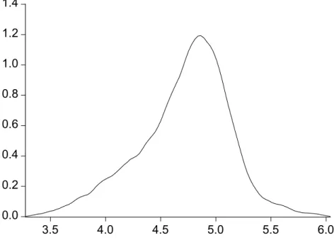
φ = 0.075, and bg = 0.014. To get some idea of how much productivity varies across countries for that speciÞcation, we computed a kernel-density estimate of lndAi, displayed in Figure 1. The features of productivity are:
(i) as in Islam, it can vary substantially across countries, with the ratio
exp³lndAmax ´
/exp³lndAmin ´
= 8.66; (ii) it is slightly skewed; and, (iii) the near-Normal shape of the density in Figure 1.
4
On The Nature of Output-per-worker
In-equality
4.1
Variance Decomposition of Output per Worker
To understand the relative contribution of inputs and productivity to the variance of output worker, two variance-decomposition exercises are per-formed. Initially, we take 1985 variables and disregard the uncertainty in parameter estimates, using α = 0.420, φ = 0.075, and g = 0.014. The Þrst exercise is a naive decomposition, because in it we disregard the fact that part of the variation of the capital-labor ratio is due to productivity vari-ation across countries. The second exercise follows Hall and Jones(1999), among others, rewriting the production function per-worker in terms of the capital-output ratio. This is a way of coping with the endogeneity problem. We show that the decomposition performed by Hall and Jones has a natural interpretation in terms of distortions to capital accumulation.
In the “naive” decomposition, given the structural model in 1985 with its error term ηi replaced by its unconditional expectation (zero), we have:
lnyi = lnAi+αlnki+ (1−α)(φhi+g·1985). (13)
We decompose the variance of (the log of) output per worker in 19856 (lny i)
in terms of (the log of) productivity (lnAi), (the log of) capital per worker
(lnki), and (the level of) human-capital per-worker(hi).
This exercise is naive because it treats each factor as exogenous in cal-culating the variance decomposition. This is particularly troublesome for physical capital, since part of its variation may be induced by productivity variation; see the discussion in Hall and Jones(1999, p. 88). Indeed, for a given investment rate, an exogenous increase in productivity will increase the incentive to accumulate capital in the long run, raising the capital per-worker ratio. Hence, part of the impact of physical capital on output is induced by productivity, and this is not taken into account in performing the
Þrst exercise.
To cope with this problem, Hall and Jones proposed performing the de-composition in terms of the capital-output ratio. The production function is
6We used 1985 because it is the last year in our sample. The same exercise was actually
rewritten as:
Yi
Li
=A
1 1−α
i Hi Li µ Ki Yi
¶α/(1−α)
, (14)
where, in this case, Hi =Liexp (φhi). Taking logs of (14):
lnyi =
1
1−αlnAi+φ(hi+g·1985) +
α
1−αln
µ
Ki
Yi
¶
. (15)
This formulation allows decomposing the variation of output per-worker into variations of productivity, human capital, and the capital-output ra-tio. Moreover, the effect of productivity on capital cancels out with that on output. Hence, variations in the capital-output ratio are free from the effect of productivity on the capital measure, answering the endogeneity problem raised above.
Hall and Jones argue that in the balanced-growth path the capital-output ratio is proportional to the investment rate, which suggests a natural inter-pretation for the decomposition based on (15). It turns out that we can also interpret it in terms of the distortions to capital accumulation present in each country. First, assume that the net return to capital is the same across countries (r). Implicitly, this relies solely on free capital mobility. We can
Þnd, for each country, its (dynamic) distortion to capital accumulation (τi)
by solving the following equation:
α(1−τi)Aikα−1
i exp [(1−α)φhi] = δ+r, or, (16)
(1−τi) =
µ
Ki
Yi
¶
·δ+r
α (17)
where δ is the depreciation rate of physical capital. Equation (17) implies that:
ln(1−τi) = ln
µ Ki Yi ¶ + ln µ δ+r
α ¶
. (18)
Therefore, any cross moments involving ln³Ki
Yi
´
will be identical to their respective counterparts using ln(1−τi), and the results of the variance
de-composition for ln³Ki
Yi
´
ln³Ki
Yi
´
based on (15) can be interpreted as the relative importance of dis-tortions to capital accumulation7.
As in the case of the decomposition based on (15), performing it using
ln(1−τi)solves the endogeneity problem of physical capital. Ceteris paribus,
the higher τi is, the smaller is the incentive for capital accumulation, and
hence, the smaller is the capital per-worker ratio in the long run. Therefore, part of the variation of lnki is induced by that of ln(1−τi), and performing
the analysis based on ln(1−τi) isolates a primary factor of lnki variation.
Implicitly, the decomposition based onln(1−τi)implies that there is no
(neg-ative) relationship between capital per worker and market returns — as in the standard neoclassical model — because τi equates returns across economies.
The approach based on ln(1−τi) is interesting in its own right, since
one rarely sees in the growth literature accounting exercises in terms of dis-tortions. Computation of τi for different countries allows: (i) measuring
which of those implicitly “tax” capital accumulation, (ii) classifying coun-tries according to distortions, and, (iii) performing counter-factual exercises in long-run growth, such as the ones discussed below.
Since we used panel-data techniques to estimate structural parameters, one can argue that performing the variance decomposition exercise using data on 1985 alone may “throw away” relevant information on other years. One way of taking all possible years into account is to time aggregate the basic equations used in variance decompositions, performing the latter in terms of time averages. Taking equation (15), for example, if we disregard irrelevant constants, a variance decomposition exercise can be based on:
1 T
T
X
t=1
lnyit=
1
1−α lnAi+φ 1 T
T
X
t=1
hit+
α
1−α 1 T T X t=1 ln µ Kit Yit ¶ , (19)
with a corresponding counterpart using (13). Notice that these decomposi-tion exercises take all years into account, being immune to cyclical ß uctu-ations and other effects that may change the cross-sectional distribution of relevant variables.
7A caveat to this approach is that we could think of distortions as simply how much the
4.2
Variance Decomposition Results
Table 4 presents the results of the variance-decomposition exercises using 1985 data. In the “naive” decomposition, the variance of productivity, phys-ical capital, and human capital account respectively for 21%, 49% and 2% of the variance of output per-worker. The remaining 28% is accounted for by the covariances between these factors. With all caveats in mind, physical capital variation can be an important factor explaining output-per-worker variation. Also, the relative importance of productivity is undeniable.
< include Table 4 here>
Quantitative results change considerably once physical capital is treated endogenously as in the decomposition used by Hall and Jones(1999), i.e., equation (15). The second line of Table 4 shows that productivity alone explains 54% of the variance of lnyi. Human capital explains 5%, and the
capital-output ratio explains 21%. These numbers are very different from those of the previous exercise, showing that, when the indirect effect of pro-ductivity on capital is accounted for, propro-ductivity explains about one-half of the variance of lnyi, rather than one-Þfth. The last row of Table 4 presents
the results of the variance-decomposition exercise, based on equation (15), when we restricted the number of countries to include only the 5 richest and 5 poorest in our sample. Productivity differences are still the main reason for income dispersion across countries.
We perform robustness checks on the results in Table 4 Þrst by running variance decompositions of output per worker for all years we have actual data on human capital (Þve year intervals, starting in 1965). Results based on 1985 data were virtually unchanged. Most year-to-year changes were of about one percentage point, and, with a few exceptions, not larger than six percentage points. Next, we decomposed the variance of 1
T
PT
t=1lnyit using
equation (19). Again, lnAi accounts for most of the variation of T1 PTt=1lnyit
— 56%, followed by 1 T
PT
t=1ln (K/Y)it — 24% and then T1
PT
t=1hti — 5%. The
Our results are similar to those in Hall and Jones(1999) and Klenow and Rodriguez-Clare(1997). This can be expecteda priori for two reasons. First, these authors use a mincerian speciÞcation for the production function. As we showed here after extensive econometric testing, this speciÞcation should be the one used in growth-accounting exercises. Second, our estimated para-meter values are very close to those used by these authors in their calibrated exercises. Again, our econometric results show that their choice of parameter values in calibration is sensible. Comparing our results to theirs shows the following: the variance decomposition of model BK4 in Table 2 of Klenow and Rodriguez-Clare — their preferred model — found productivity explaining 66% of output per worker variation vis-a-vis only 34% for inputs. Given the zero covariance restriction in their exercise, if we impose it in ours (Table 4), weÞnd almost the same values, 67.5% and 32.5%, for productivity and inputs respectively. Hall and Jones, compare the 5 richest to the 5 poorest countries. They Þnd that productivity alone explains 67% of income variation. Again ignoring covariances, our results in Table 4 show that productivity explains 62.3% of the income difference of these two groups.
4.3
Productivity, Distortions, and Counter-Factual
Ex-ercises on Long-Run Growth
Before ourÞnal exercise on “the nature of output-per-worker inequality across nations” is performed, we present basic statistics for a select group of coun-tries on estimated total factor productivity — lndAi, distortions to capital
accumulation — τi and human capital measures — hi, relative to their U.S.
counterparts. Results are reported in Table 5.
< include Table 5 here>
times smaller than that of the U.S. economy. Moreover, the U.S.S.R. and Czechoslovakia are respectively only 43% and 37% as productive as the U.S. Also, the productivity of the U.S.S.R. is the same as Ghana’s. The second group is composed of some Asian countries: Japan, Taiwan, and South Korea all have below-average productivity by world standards.
Rich (and more educated) nations distort capital accumulation less than poor (and under-educated) nations do. For instance, while the average per-capita income of the group of 20 countries with the highest estimated dis-tortion is only 7.1% of the USA, that of the 20 least distortive countries is 59.2% income in the U.S. However, since the correlation between ln (1−τi)
and lnAi is close to zero (actually 0.08), economies that are very good at
combining inputs (i.e., are highly productive) do not necessarily have the right incentives to boost capital accumulation. Ex-communist countries and some Asian countries have small distortions and are relatively unproductive; e.g., Japan, Korea, and Taiwan. For the latter group, the case of Japan is very interesting: its productivity is below world average but its distortion is the third lowest amongst all nations (it is negative — a subsidy — as a matter of fact). These Þndings are consistent with Young’s(1995) result that the good growth performance of some Asian countries in the recent past was mostly due to factor accumulation, not productivity.
Table 6 displays a counter-factual exercise on long-run growth, which might help in understanding the nature of income inequality across nations. The second column displays 1985 output per worker (relative to the U.S.) — Yi/YU S. The third column shows relative income corrected for τi, i.e.,
where countryiis given the sameτ as the U.S. economy. The fourth column corrects for human capital and τ, i.e., where country i is given the same τ
and human capital as that of the U.S. economy8.
< include Table 6 here>
Most of the time, relative output increases when we allow a country to have the U.S. τ and h measures; see the case of Argentina, Mexico, and particularly Mozambique, where output per worker increases by almost ten times. However, there are exceptions: for Japan and the ex-communist coun-tries, output decreases when we allow them to have the U.S. distortion. Given
8A different way to look at the fourth column of Table 6 is to regard it as the relative
that the education level observed in these countries is similar to the U.S. level, the fourth column shows that, if it were not for capital accumulation, output per worker in these countries would be almost half of the actual difference.
There are groups of countries, such as India and Niger, where the increase in relative income brought about by the reduction of τ and improvement in education is not very large. In this case, most of the difference between them and the U.S. is due to productivity differences. European countries which have output per worker close to that of the U.S., such as the Netherlands, Austria, and France, would not change much either, but for different reasons: their τi, hi and ln (Ai) are already very close to those of the U.S. economy.
However, this pattern is not uniform across Europe: if Spain had the same in-centives to capital accumulation and educational level as the U.S., its relative output would jump from 45% to 73% of the latter’s.
It deserves note that even after correcting for factor differences across countries, there still remains a large income disparity left unexplained. On average, output per worker of the 95 nations in our data set is 29% of that of the U.S. After substituting their τi and hi with the corresponding values
of the American economy, the average output per worker increases to only 48% of the U.S. output; the rest corresponds to total factor productivity differences.
5
Conclusion
In this paper we estimate and test two alternative functional forms, that have been used in the growth literature, representing the aggregate production function for a panel of countries: the extended neoclassical growth model — proposed by Mankiw Romer and Weil(1992), among others, and a mincerian formulation of schooling-returns to skills — e.g., Mincer(1974) and Wills(1986) — recently incorporated into the growth literature by Bils and Klenow(2000), and Hall and Jones(1999).
Our evidence rejects the extended neoclassical growth model in favor of the mincerian speciÞcation, with an estimated capital share of about 42%, a marginal return to education of about 7.5% per year of schooling, and an estimated productivity growth of about 1.4% per year. Previously, several authors have made the case for the mincerian form based on microeconomic evidence; see Hall and Jones, Klenow and Rodríguez-Clare, and Bils and Klenow. The present study conÞrms the appropriateness of this approach from a macroeconomic perspective, reconciling our estimate of the marginal return to education with those obtained in micro studies. This result in-creases our conÞdence that the mincerian speciÞcation should be used in future studies and also the conÞdence with which we regard the growth-accounting results based on it.
In panel-data regressions, productivity was preferably modelled as aÞxed effect, varying across countries but not across time. Regression results show that productivity estimates vary considerably across countries. In growth accounting exercises, once the endogeneity of physical capital per worker is taken into account, differences in productivity emerge as a fundamental vari-able in explaining why output per worker varies so much across countries, a result along the lines of Hall and Jones and of Klenow and Rodriguez-Clare. Thus, the conclusion that inputs alone can explain the variation of output per worker can be called into question. However, our decomposition exer-cises show that there is not a single cause for poverty, and some productive economies with either poor incentives to capital accumulation or low levels of schooling, or both, can have low levels of per-capita income.
References
[1] Barro, R. and J. W. Lee, 1996. ”International Measures of Schooling Years and Schooling Quality, ” American Economic Review, 86, 2, pp. 218-223.
[2] Basmann, R.L., 1960, “On Finite Sample Distributions of General-ized Classical Linear IdentiÞability Test Restrictions,” Journal of the American Statistical Association, 55, pp. 650-659.
[4] Bills, M. and P. Klenow 2000. “Does Schooling Cause Growth?,”
American Economic Review, 90, 5, pp.1160-1183.
[5] Chari, V. V., Kehoe, P. J. and E. McGrattan. 1997,“The poverty of nations: a quantitative investigation.”Research Department Staff Re-port 204, Federal Reserve Bank of Minneapolis (Revised October 1997).
[6] Cooley, T. and Prescott, E., 1995, “Economic Growth and Business Cycles,” in Cooley, T. and Prescott, E. (eds.), “Frontiers of Business Cycle Research.” Princeton, Princeton University Press.
[7] Davidson, Russell and James G. MacKinnon, 1993, “Estimation and Inference in Econometrics,” Oxford: Oxford University Press.
[8] Feldstein, M. and C. Horioka, 1980, “Domestic Saving and Inter-national Capital Flows.” The Economic Journal, vol. 90, pp.314-329.
[9] Gollin, D., 1997, ”Getting Income Shares Right: Self Employment, Unincorporated Enterprise, and the Cobb-Douglas Hypothesis, Mimeo, William College.
[10] Hall, R.E. and C. Jones, 1999, “Why do some countries produce so much more output per worker than others? ” Quarterly Journal of Economics, February, Vol. 114, pp. 83-116.
[11] Hausman, Jerry A., 1978, “SpeciÞcation Tests in Econometrics,”
Econometrica, vol. 46, pp. 1251-1272.
[12] Hsiao, C., 1986, “Analysis of Panel Data,” Econometric Society Monograph Series.
[13] Islam, N., 1995,Growth Empirics: A Panel Data Approach,Quarterly Journal of Economics, vol. 110, pp. 1127-1170.
[14] Klenow, P. J. and A. Rodríguez-Clare, 1997, “The neoclassical revival in growth economics: has it gone too far? ” NBER Macro-economics Annual 1997 eds. Ben S. Bernanke and Julio J. Rotemberg, Cambridge, MA: The MIT Press, pp. 73-103.
[16] Mankiw, N. G., Romer, D. and D.Weil. 1992, “A Contribution To The Empirics Of Economic Growth.”The Quarterly Journal of Eco-nomics 107 (May): 407-437.
[17] Maddison, A., 1995, “Monitoring the World Economy: 1820-1992,” Paris: OECD.
[18] Mincer, J., 1974, Schooling, Experience, and Earning, National Bu-reau of Economic Research, distributed by Columbia University Press.
[19] Prescott, E., 1998, “Needed: a Theory of Total Factor Productivity,”
International Economic Review, vol. 39(3), pp. 525-551.
[20] Psacharopoulos, G., 1994, ”Returns to Investment in Education: A Global Update,” World Development, 22(9), pp. 1325-1343.
[21] Sargan, J. D., 1958, “The Estimation of Economic Relationships using Instrumental Variables,” Econometrica, vol. 26(3), pp. 393-415.
[22] Summers, R. and A. Heston, 1991, ”The Penn World Table: An Ex-panded Set of International Comparisons”, 1950-1988, Quarterly Jour-nal of Economics, 106, May, pp. 327-368.
[23] Willis, R. J., 1986, “Wage determinants: a survey and reinterpreta-tion of human capital earnings funcreinterpreta-tions.” in Handbook of Labor Eco-nomics, volume 1, eds. Orley Ashenfelter and Richard Layard. North-Holland. Chapter 10: 525-602.
6
Figures and Tables
0.0 0.2 0.4 0.6 0.8 1.0 1.2 1.4
3.5 4.0 4.5 5.0 5.5 6.0
Table 1: Estimates of the Mincerian Growth Model Log-Level Model
Estimated Equation: lnyit = lnAi+αlnkit+ (1−α)(φhit+g·t) +ηit,
Parameters/Statistics Depreciation Rates(δ)
3% 6% 9% 12% 15%
α 0.4038 0.4124 0.4195 0.4183 0.4176 (t-ratio) (66.58) (70.62) (71.92) (73.80) (75.00)
φ 0.0916 0.0870 0.0753 0.0772 0.0760 (t-ratio) (13.69) (13.64) (12.05) (12.93) (13.24)
g 0.0140 0.0138 0.0140 0.0140 0.0142 (t-ratio) (22.61) (23.44) (24.60) (25.63) (26.90) Box-Cox θ= 1 (p-value) 0.7520 0.7153 0.7517 0.9112 0.7743 Box-Cox θ= 0 (p-value) 0.0000 0.0000 0.0000 0.0000 0.0000 Hausman Test (p-value) 0.0000 0.0000 0.0000 0.0000 0.0000 Sargan: Rejections at 5% 21/95 20/95 15/95 14/95 14/95
lnAi = lnA,∀i (p-value) 0.0000 0.0000 0.0000 0.0000 0.0000
Table 2: Estimates of the Extended Neoclassical Growth Model - Double-Log Model
Estimated Equation: lnyit = lnAi+αlnkit+βlnhit+ (1−α−β)·g·t+ηit,
Parameters/Statistics Depreciation Rates (δ)
3% 6% 9% 12% 15%
α 0.4097 0.4217 0.4325 0.4287 0.4273 (t-ratio) (68.77) (72.95) (74.60) (75.59) (76.09)
β 0.0278 0.0320 0.0215 0.0256 0.0227 (t-ratio) (2.20) (2.61) (1.76) (2.11) (1.87)
g 0.0204 0.0195 0.0187 0.0194 0.0197 (t-ratio) (51.44) (50.24) (49.40) (53.09) (55.70) Hausman Test (p-value) 0.0000 0.0000 0.0000 0.0000 0.0000 Sargan: Rejections at 5% 22/95 19/95 21/95 17/95 17/95
Table 3: Estimates of the Models in Box-Cox Form Estimated Equation: lnyit = lnAi+λ1lnkit+λ2
³
hθ it−1
θ
´
+λ3·t+ηit,
Parameters/Statistics Depreciation Rates(δ)
3% 6% 9% 12% 15%
λ1 0.4038 0.4125 0.4195 0.4186 0.4181
(t-ratio) (66.61) (70.69) (71.84) (73.69) (74.66)
λ2 0.0571 0.0540 0.0462 0.0458 0.0419
(t-ratio) (6.11) (5.91) (5.07) (5.14) (4.89)
λ3 0.0084 0.0081 0.0082 0.0081 0.0083
(t-ratio) (21.10) (21.79) (22.86) (23.85) (25.03)
θ 0.9742 0.9685 0.9692 0.9894 1.0302 (t-ratio) (11.68) (11.17) (9.61) (9.96) (9.92) Box-Cox θ = 1(p-value) 0.7571 0.7166 0.7602 0.9151 0.7711 Box-Cox θ = 0(p-value) 0.0000 0.0000 0.0000 0.0000 0.0000
Table 4: Variance Decomposition of Output per Worker (1985) in Terms of Different Factors
Var. Decomposition of lnyi (in 1985) % of variance due to factor
lnAi ln
³
Ki
Yi
´
lnki hi PCov.
orln (1−τi)
“Naive,” Eq. (13) 21 49 2 28
Equation (15) 54 21 5 20
Table 5: Relative Productivity Estimate for Selected Countries (U.S.=1.00) Factors and Productivity Relative to the U.S
Country Ai
AU S τi τU S
hi
hU S
Iran 1.23 1.61 0.28 Netherlands 0.93 0.68 0.73 Canada 0.92 0.79 0.87 Spain 0.88 0.70 0.54 Argentina 0.81 1.18 0.61 Brazil 0.71 1.13 0.29 Chile 0.67 1.24 0.56 Japan 0.58 -0.11 0.76 Korea 0.56 1.02 0.75 Indonesia 0.44 1.35 0.35 U.S.S.R. 0.43 -0.64 0.83 Ghana 0.43 2.11 0.31 India 0.36 1.55 0.32 Kenya 0.29 1.41 0.29 Romania 0.23 0.05 0.68 Malawi 0.20 1.39 0.24
Table 6: Relative Output of Selected Countries in Counter-Factual Analysis
Country/Statistics Yi/YU S Yi/YU S Yi/YU S
(Uncorrected) (τi =τUS) (hi =hU S,and τi =τU S)
Argentina 0.32 0.53 0.64 Brazil 0.24 0.34 0.48 Mozambique 0.05 0.34 0.55
Niger 0.03 0.08 0.13
India 0.06 0.10 0.15
Japan 0.71 0.33 0.38
U.S.S.R. 0.42 0.21 0.23
Spain 0.45 0.58 0.73