. LLセfundaᅦᅢo@
" aETUUO VARGAS S L \ 1I :'\ .:\ R I ( )
"-DL": PI-S()l"1 "- \ LCO:'\O\II( \
-.
EPGE
Escola de Pós-Graduaçao em Economia
UEtfect.
oI
Trade
Polia)' on Technolol)'
Acloptlon and Inveltment"
Prof. Arilton Teixeira
(PUCIMG)
LOCAL
Fundação Getulio Vargas
Praia de Botafogo, 190 - 100 andar - Auditório
bATA
14/10/99 (5- feira)
fuセjdエ@ ('""" イセセAB@ '(I GNGセ@
PC?AS
biXlャgセN⦅N@ " .. ' 'J ; ;..-, .:'"-:,,,, ... GZ[セセQPnseエNs@
ABf.
! {)
JJ
GC< .•"
-,
Effects of Trade Policy on Technology
Adoption and Investment*
Arilton Teixeira
TSeptember
RTセ@1999
Abstract
This paper studies the consequences of trade policy for the adop-tion of ne\\" technologies. It develops a dynamic internaadop-tional trade mo deI with t\VO sectors. \Vorkers in manufacturing decide if new tech-nologies are used, capital o\\"ners then choose investment. We analyze three different arrangements: free trade, tariffs, and quotas. In the model economy, free trade as well as tariffs guarantee that the most productive technology available will be used. In contrasL under a quota the most productive technology available will not be used at all times. Further, in the latter case investment and the capital stock are smaller than in the former one. Finally, there exists parameter values for \vhich the computed difference in GDP is a factor of thirty.
1
Introd uction
An important question in grO\vth and development is why the technological
leveI (Total Factor Productivity - TFP) differs over time and across
COUll-tries. To answer this question we will start with the arguments of Prescott
r?].
First, the observed difference in productivity across countries is not explained by the difference in the capital-labor ratio: instead the differences in the
*This paper is part of my PhD clissertation. I aro greatfull to Ed Prescott. Tim Ke-hoe, Berthold Herrendorf, Ron Ed'wards, J. C. Conessa and Carlos Diaz. As usual, the remaining mistakes are mine.
capital-labor ratio are caused by differences in total factor productivity. Sel ond, the differences of productivity across countries by itself are a result of different growth rates of TFP over time and across countries. Third, the knowledge that is being used by the \vorkers of the richest countries is available to be used by the workers of any other country, in particular poor countries.
The goal of the model developed here is to explain why different countries use different technologies. We argue that a combination of two factors can
explain whether or not a country adopts a ne\v technology: (i) its internaI
institutional arrangement: (ií) its trade polic}·. In particular, the internaI
institutional arrangement determines whether there are groups of interest that can resist the adoption of new technologies. The trade policy determines whether these groups find it optimal to resist the new technologies. For simplicity, I take as given that there are groups of interest that can block technologies and study how the choice of trade policy affects their decision problem whether or not to resisto
To model this idea, I develop a two-sector grO\vth model with
interna-tional trade. In both sectors there is exogenous technological progress: in
each period a new and more productive technology becomes available. \Vhile
in both sectors, there is perfect competition, the technology is different. セャッイ・@
specifically, in one sectoL the inputs into the production process are unskilled labor only, which any worker can supply. Hence, I assume that workers in that sector are not organized and cannot resist the introduction of new
tech-nologies. In the other sector, the production function uses both labor and
capital. \Vhile labor may be unskilled or skilled, the most productive tech-nology can only be operated by skilled labor. Skilled workers are therefore assumed to act in coalition, so they are able to resist new technologies. Given that skilled workers have chosen the technology that can be used, the capital O\vners non-cooperatively decide how much to invest.
The main results are: (í) with free trade, firms will always use the most
productive technology available: this is also true with tariffs; (ií) with a quota, firms generally will not use the most productive technology available; (iii) investment and the capital stock are smaller Vvl.th a quota than with free
trade: (ív) there exists parameter values for which the difference between
•
of new technologies because given the price of its product, producing most efficiently maximizes its income (and thus their utility). Since under a tariff, the domestic price equals the international price times a constant factor, it does not break the link between the domestic and international price and so the same argument as under free trade applies. In contrast, if a quota is introduced then the domestic price becomes independent of the international price. In this case, skilled labor can increase the relative price of the good produced in its sector by blocking the use of a new technology. This can increase the income of skilIed labor and so be in its interest if technological progress is not too rapid and skilIed labor is a relatively smalI group that faces a relatively large internaI market. The intuition is that on one hand, if the technology advances too rapid then the opportunity cost of not using the most advanced technology is too large. On the other hand, if the domestic market is relatively smalL then the gain from manipulating the domestic price is not sufficient relative to the cost.
The ideas developed in this paper are related to those of Parente and
Prescott
[?],
Parente and Prescott[?],
and Holmes and Schrnitzr?].
The keyidea of these papers is that the ability to invest and adopt new technologies
determines the grO\vth rate of an economy. vVhile Parente and Prescott
r?]
focus on barriers to investment coming from the internaI structure of the
economy, Parente and Prescott
[?]
shows how monopolies can interfere inthe adoption of ne\v technologies. Holmes and Schrnitz make the comple-mentary point that organized interest groups can have the power and find it in their interest to resist the adoption of new technologies. VVhile some of my conclusions are similar in spirit to those of Holmes and Schmitz, my model is more general. In particular, their model has two periods only whereas I develop an infinite horizon modeL Besides, I introduce a capital good. These features alIow me to go considerably further than Homes and Schrnitz in that I can generate artificial time series that can be compared with the data.
This paper is divided into five sections (including this introduction). In Section 2, we look at some empírical evidence to support our main thesis. In
Section 3, we develop a IDO deI that studies the adoption of technology. First
..
2
Some Evidence
In this part of the paper we will show some empirical evidence that supports the main ideas behind this paper. First, the technological leveI differs over time and across countries. Second, it is the exposure to externaI competition that stops groups from exercising their resistance to new technologies. There-fore, it is the exposure to externaI competition that explains the difference in the technological leveI and productivity across countries.
Here we wilI not show evidence of resistance to the adoption of new nologies across countries or that this resistance succeeds in stopping the tech-nological progress in the countries. This evidence has been showed by
Par-ente and Prescott [?], Holmes and Schmitiz [?], :"IokYT [?], :\;IokJT [?] and
?\IokJT
r?].
In particular, Parente and Prescottr?]
and Holmes andSchmi-tiz [?] have summarized results. The basic idea behind these papers is that
technological progress affects groups of agents differently. Some groups have their income increased by technological progress and some groups have their income reduced (at least in the periods immediately after the introduction of the new technology). In this case, the group harmed by the technological progress has incentive to resist the adoption of new technologies.
Harrigan
[?]
and DolIar and Wolf[?]
estimated the differences in TFPacross countries.1 Harrigan
[?]
estimated differences in TFP across tencoun-tries and six induscoun-tries. More specificalIy, he estimated the difference be-tween the TFP of each industry of each country with respect to the TFP of that industry in the USA. The period studied is 1980-89. The countries used in this study are: Australia, Canada, Finland, Germany, Italy, Japan, Netherlands, Norway and the USo The industries include the following: non-electrical machinery, office and computer equipment, non-electrical machinery, radio, TV and communications, motor vehicles, ship-building, aircraft and other transportation equipments. The US has a higher TFP in alI but one industry. The exception is the electrical machinery industry where Japan, Australia and Canada have higher TFP than the "CSA.
DolIar and Wólf [?] estimated differences of TFP in manufacturing using a
sample of twelve countries: Australia, Belgium, Canada, Denmark, Finland, France, Germany, Italy, Japan, Netherlands, Norway, Sweden, the United
-,
Kingdom and the USo The period studied is longe r than the one covered by
Harrigan
[?]:
1965-85. At this more aggregate leveI the US has a higher TFPthan any other country in the sample and for the whole period.
At this point we would like to have estimations of TFP for some develop-ing countries to compare \vith the TFP of developed countries. But because of lack of data these estimations are not available. ='Jonetheless, we are taking the numbers presented above as an indicator of the existence of differences of TFP between less developed countries and developed countries.
Given these studies that estimate the differences of TFP across countries, let us show some empirical evidence for the second point listed in the
begin-ning of this section. It is the exposure to e:\.-ternal competition that explains
differences in the technological leveI and productivity across countries.
Baily and Gersbach
[?]
studied 9 industries in 3 countries: Germany,Japan and the USo These industries account for 15% to 20% of the employ-ment and 17% to 22% of the value added in the manufacturing sector. The
basic conclusions of their study are: (i) physical capital can partially explain
the differences of productivity in each industry across countries: however, the major part of the differences in productivity is explained by differences in the
way that labor tasks are organized and the product design: (ii) there is not
enough evidence to justify differences in productivities by differential access
to proprietary technology; (iii) domestic competition is not enough to make
domestic firms achieve the highest productivity; (iv) the greater the exposure
of the domestic firms to the highest productivity firms the smaller was the difference in productivity. International trade and foreign investment force the adoption of the best practice or highest productivity production processo
Baily
[?]
studied service industries, airlines, retail banking,telecommuni-cations and general merchandise retailing in France, Germany, J apan, the VK
and the USo Again, the conclusions do not differ from Baily and Gersbach
r?].
Regulations prevent adjustment in the industries and generate a non com-petitive market. Once more, the cost of these regulations are industries with low productivity (compared with the world best practice producer).
The last evidence that we present here comes from Luzio
[?]
who studiedthe microcomputer industry in Brazil from the beginning of the seventies until the beginning of the nineties.
Since the beginning of the seventies, the microcomputer industry
(in-cluding software) in Brazil has been highly protected and regulated2 . The
"
-.
support for protection at first was given by the military because the potential use of computers in weapons and defense equipments.
By the beginning of the eighties the protection of the microcomputer in-dustry reached its highest leveI with the approval of the Informatica La'w: imports were prohibited and the exceptions \Vere analyzed by a special gov-ernrnent agency created just to regulate the microcomputer industry, Special Secretariat for Informatica (SEI).3
The consequences that come from this long period of protection and reg-ulation fonow the lines of the studies analyzed before. "Neither the Brazilian micro-electronics nor the soft\vare industry developed as expected by SEI", " ... the restrictions only increased the technological gap and the pricejquality difference between domestic and foreign Informatica products"4. One of the reasons for this technological gap was the lack of investment in R&D and physical capital. Instead to generate an increment in the amount invested in this industry, protection had an opposite effect. "According to SEI there was little R&D related to production". Besides. "a major part of R&D expenses
were directly or indirectly imposed by regulation" . 5
By the end of the eighties and the beginning of the nineties the Brazilian industry of micro-electronics and software "vas producing obsolete computers using obsolete technology. The more sophisticated computers produced in Brazil when compared with "similar" ones produced in the US would cost between 5 to 6 times moré.
3
The Madel
In this section we wiU develop a model with physical capital.7 \\Te introduce a
capital good in the model, but only a certain type of agent can own capital. \\Te have two reasons to introduce physical capital in this way. First. we \vant to see how resistance to adopt new technologies affects investment and
two decades.
3See Luzio
r?,
page 8J.4See See Luzio セ_L@ pages 12-13]. 5See Luzio イ_セ@ pages 94-95 ].
6See Luzio イ_セ@ page 110].
..
the capital stock. Second, \ve \vant to study how the resistance to new
technologies affects the capital owners income.8 We \,'ould like to stress two
ways that the resistance to new technologies affects and benefits the capital O\vners. First, it aUows the capital owners to reduce investmenL increasing the part of their income that can be used for consumption. Second, the resistance to new technologies in one sector increases the relative price of the good produced by this sector. Given the productivity of capitaL the increment in the relative price of the good increases the rental price of capital. Thus, capital O\vners (and workers that resist) can be better off if there is blocking of new technologies.
In this section we \viU see that even if technological progress is faster
in one sector (that I will call a manufacturing sector), protection wiU not
increase the gro\vth rate of the economy. In fact, protection generates a
bigger manufacturing sector but it reduces the growth rate of the economy. That is, protection just generates an inefficient and stagnated manufacturing sector.
There are three types of agents, i = 1,2,3 and the measures of the type
i are Ài
>
o.
A type i=
L 2 agent is endO\ved with one unit of time of laborof type i. In the third group, group of type 3, each agent owns capital that
they rent to firms. This group has measure one. :Vloreover. just type 3 can O\vn capital. The capital owners do not \vork. They are not endowed with one unit of time of labor in each period. Their income is the rent paid by the firms to use capital services. Their preferences are ordered by the same utility function of the other agents.
At each date, there are two goods y and z. Good y is food and good z
is a manufacture. Good z can be used as consumption good or as capital
good. The production of good z uses labor and capital services as inputs.
The production of good y uses only labor input. There is no borrowing and
lending and no capital accumulation.
As we said before, the reason to introduce a group that owns capital, instead to aUow group of type 1 and group of type 2 to be the o\vners is to isolate the effects of technology blocking over the capital income and over
the labor income. \\ie want to stress that workers of type 2 wiU be better
off if they block the ne\\' technology even if they do not have any capital income. Since capital income aIs o increases if there is blocking, this could
jeopardize the labor income effect over the decision to block the adoption of new technologies.
The period commodity space in the mo deI is L = R6 \'lith a point in L
being x
=
(y, z, ly' Izl, IZ2, k). This different kinds of labor depend on \'lhosupplies and the industry that uses the labor (it wiU become clear later on
in the paper). It should be stressed that there is no differentiation beh'leen
workers of type 1 and 2 in the y industry.
The consumption set of the agent of type 1 is
(1)
The consumption set of the agent of type 2 is
(2)
The consumption set of the agent of type 3 is
(3)
\,ve abuse the notation and use k to denote both stock and fiow of capital
service, as a unit of capital provides a unit of services. A type 3 agent with k
units of capital good can supply k of capital services. The amount supplied,
kS
, is smaUer or equal to k .
• Preferences
The period utility function for aU types is
(yo. zl-o.)p u(y,z)
=
"':"';"""'---'--p (4)
where y, z セ@ O and p:S; 1. Besides, we are assurning that preferences are
time separable. In a dynamic environment preferences are represented by
( o. l-o.)P
t
pt Yt Ztt=O p
(5)
• Technologies
since it does not use capital as input. The same is true for foreign trade technology.
The production set of good y is
(6)
where 7í
>
1. Equation (6) implies an exogenous technological progress inthe y production sector. Besides, Equation (6) implies that both kinds of
workers have the same productivity in the y sector.
The second technology produces good z. Its production set is
Xda, b)
=
{x E L+ : z ::; セH。@ ォセ@ ャセャャャ@+
'[b kg ャセRQQL@ k1+
k2 ::;k,
y=
O} (7)where í'
>
Lk
/
K is very small and K is the stock of capital in the economy.Elements a
<
b are integers that index the z-production in a period. Theseelements are determined by past policy decisions. vVe assume that セヲ@
>
7í.The third is a foreign trade technology that transforms one good into the
other at a rate P;t in period t. Its technology set is
(8)
X6(t) implies that there is no borrowing or lending and no transportation
cost. Since the externaI prices of goods y and z are exogenous (and good y
is a numeraire), we \vill assume that the externaI price of good z at period t
is given by
(9)
The reason v;hy ownership of technologies is not considered is that alI technologies displays constant return to scale. Therefore, profits in equilib-rium must be zero .
• Policy Arrangement
The integers a and b, where a
<
b index the technology set X5(a, b), whichproduces good z. These integers a and b at date t belong to the set {O, ... ,
t-I, t}.
During the period t, type 2 decides what technology to use next period;
that is, type 2 chooses b' E {b, ... , t, t
+
l}.
If b' > b, that is a bettertype 2 choose a better technology the type 1 gain access to the technology
that the type 2 \Vere using. If the type 2 choose to continue using the b
technology, type 1 does not get access to the b technology9 .
• Definition
\;V'e will say that the group of ty-pe 2 is blocking the adoption of ne\v
tech-nologies or there is blocking of technologie8 if b
<
t .• Timing
In the beginning of each period workers of type 2 get together and define
the technology index that they wiU use ne:x.1: period. This choice becomes public knowledge and it cannot be changed in the future. Once type 2 has
announced their decision, non cooperatively t)-pe 3 chooses k'. It should be
noticed that there is no private information.
3.1
Dynamic Equilibrium
This is a discrete time dynamic game with two stages in each period. At
the first stage group of type 2 chooses b'. At the second stage members of
groups 3 chooses k' non cooperatively and price and allocations are
deter-mined competitively.
\Ve restrict our attention to :'larkov equilibrium which is symmetric with
respect to members of group 3.10 The state variable, at the beginning of a
period, becomes (8, K), where as before 8
=
(a, b, t).ll The integers a, b andt index the technology sets X4(t), X5(a, b) and X6(t). The maximization
problem of the agent of ty-pe 1 as well as the maximization problem of firrns
do not change with the introduction of capital.
The maximization problem of a ty-pe 3, like the maximization prob-lem of type 2, is a dynamic probprob-lem. At the beginning of the period the
relevant state variable for a type 3 is (8, K, k). To study the
maximiza-tion problem of ty-pe 2 and the maximization problem of a ty-pe 3 we will
9In period zero, since no technology has being abandoned, we are assuming that type 1 works in the production of good z with technology ex-I.
10 See ?-'Iaskin and Tirole :?j.
,
break the equilibrium in two parts; a period competitive equilibrium and a
:\!arkov perfect equilibrium. Given (s, K) there is a set of price functions
p
=
{p
y=
1, Pz, wy, w z 1, 7L'z2, r} and allocation functions for consumers andfirms that form a period competitive equilibrium. Given these prices and
state variables (s, K, k), the indirect utility correspondence of each type is
determined. That is, these correspondences will just depend on these state
variables. In addition, for the structure considered here, these
correspon-dences \vill be single value and they will be functions.
Given 5, the space ofthe state variables, and the assumed policy
arrange-ment, type 2's choice set of Si is denoted T( s) where12
T ( s )
= { (
ai, bl, ti) : ti = t
+
1, b l::; t
+
1, ai=
a if
bl=
b arai = b i
f
bl>
b}
In each period the game is analyzed using backward induction from stage
2 to stage 1. In the last stage of a period the state variables of the economy
are (s, K, Si). Firms of both sectors have a static problem. With a Markov equilibrium. the objective function for a type 1 is simply
r (yOzl-o)P
Úl(X) = u(y, z)
=
-p The problem of a type 1 is not dynamic.I am following convention used in the national income and product ac-count and more generally in macroeconomics rather than those used in math-ematical economics. Vhth the convention used here all quantities are positive
(or zero). The price of the factor inputs are negative. The rental price are the negatives of these and therefore positive.
The ma.ximization problem of a type 2 is dynamic. First, Iet U2(x) =
u(y, z). At the second stage their objective is
[;2(S, K, Si) = max{U2(x)
+
;3V2(SI, K I)}x
s.t. p(S,K,SI).
x::;
OKI
=
G3(s, K, Si)
here Ú2(s, K. Si) is the indirect utility function; V2(') is the present vaIue of
the equilibrium fiows from the next period on conditional on next period's state variables.
The problem of a type 3 is also dynamic \vhich leads to objective
U3(s. K, k, s')
=
セコセヲLサオHケL@ z - k'+
(1 - b)k)+
3V3(S', K', k')} s.t. p(s, K, s') . x:s;
OK'
=
G3(s, K, s')The k' is the individual's capital stock tomorrow and K' is the aggregate
capital stock. Remember that the z-good can be used for z-consumption
and investment. If a type 3 purchases z units of good z and chooses k' then
consumption of z-good is z - k'
+
(1 - b)k.At the first stage of the game the state variables are (s, K), type 2 group
solves the following problem,
In the first stage of period t a type 3 does not move and his payoff is
• Dynamic Recursive Equilibrium
The equilibrium that \ve are working with is a :"Iarkov equilibrium13 with
respect to the state variables (s. K). An equilibrium is the following set of
elements:
(i) price functions p( s. K, s')
=
{Py=
L pz, wy, Wzl ,''(L'z2, T};(ii) households allocations {x;(s,K,S')}T=l and x3(s,K,k,s'):
(iii) firms allocations {x;(s, kIスセ]TZ@
(iv) laws of motion k' = 93(S, K, k, s'), K' = G3(s, K, s') and s' = G2(s, K);
(v) value functions v2(s,K), v3(s,K,k);
(vi) Indirect utility functions U2(s, K, s') and U3(S, K, k, s'), such that
1) Given p(s,K,s'), (s,K,s'), (s,K,k,s') in the case of a t:ype 3 and K'
=
G3(s, K, s'), {xi}f=l solves the consumers' problem and サx[スセ]T@ solves the firms' problem;
,
2) K '
=
g3(S, K, K, Si)=
G3(s, K, Si):3) セャ。イォ・エウ@ clear:
4) G2(s, K) E argmaxs'ET(s) {U2(S, K, Si)} and
'U2(s,K)
=
U2(s,K,G2(s,K)):5) g3(S, K, k, Si) E argmax{U3(s, K, k, Si)} and
1)3(S, K. k)
=
U
3(S, K, k, G2(s, K))3.2
The Equilibrium with Free Trade
In tms section we wiU characterize the equiIibrium path of the mo deI econ-omy with free trade. \Ve assume that there are no barriers to trade and no transportation cost.
Before we go any further let us analyze more carefully how we can deter-mine the equilibrium in tms model. First, we can break the equilibrium in
two parts: a セャ。イォッカ@ perfect equilibrium and a period competitive
equilib-num.
Since we are interested in the symmetric equilibrium with respect to the capital owners, for a dynamic equilibrium we need to Iook at the interaction
between G2(s, K) and G3(s. K, Si)
=
g3(S, K, K, Si). That is, to choose thetechnology, agents of type 2 need to know how their choice \,riU affed the investment of the firms.
In what foUO\vs, to simplify the solution of tms modeL we will take the following steps. First, \ve will show that vúth free trade, no blocking is
the best strategy for type 2, that is, b = t. Tms completely characterizes
G2(s, K) (See Lemma 1). Second, given G2(K, s) and G3(s, K, Si), we will
show that there exists an optimum policy rule for type 3 g3 ( s, K, k, Si) and
that G3(s, K, Si) = g3(S, K, K, Si) (See Lemma 2). Finally, we use Lemmas
1-2 to proof the existence of a dynamic recursive equilibrium.
The first proposition of tms section shows that with free trade there is no blocking of technology.
Lemma 1 lf there is free trade, that is, every agent has access to X6(t)
,
We could state a proposition showing that there exists a value function
V2 (s, K) and a policy function G2 (s, K) for the maxirnization problem of type
2 group. But, the above lemma give us the necessary result, that is G2(s, K).
The next step is to study the type 3 behavior. \Ve will see that in a open world, that is, \vhere there is no barriers to trade, group 2 does not block the adoption of new technologies and the fums invest an amount that keeps the marginal productivity of capital constant. In other words, in an open world group 2 does not use his option to block the adoption of technology.14
Since we are working in the case of unbounded returns, we wiU not be able to use standard techniques using the variables of the original model. 15 Therefore, \ve will redefine all variables such that the solution of the max-irnization problem of the the representative fums problem is equivalent to the problem using these redefined variables. ?vIore important, this redefined problem will be solved using bounded return techniques16 .
From Lemma 1 we know that in a free trade environrnent b
=
t, smcethere is no blocking. Let!3
=
SHイゥ]セ@
li°')P andfJ
=
1](1-・IHセIゥjN@
Lemma 2 lf(i) 1:S fJ:S セH[@ (ii) jj E (0,1),' (iii) G2(s,K)
=
s'=
(t-Lt,t+1): and (iv) there is free trade, then there exists a law of motion of the
aggregate capital stock and a policy function for a type 3 where G3 (s, K, s') =
1
g3(S. K, K. s') = セLセ@ K and
Yt':"'l y;-l Yit':"'l
- - = - - = - - = í í
Yt Y; Yit (10)
Zt.:,..l Z;-'-l Zit+1 K t':"'l _1_
-- = -'- = - - = - -
= í 1-8Zt
z;
Zit Kt(ll)
In the above lemma. y* and z* are the volumes of good Y and z, respectively,
traded in the international market. 1'\ow, using Lemmas 1-2, we wiU show that there exists a recursive dynamic equilibrium.
Proposition 1 lf (i) 1 :S
fJ
:S 'Y; (ii) !3 E (O, 1): and (iii) there is free trade.then there are
14This dynamic policy equilibrium where ali variables are gro\\ing at a constant rate and the marginal producti\ity of capital is constant will be called a balanced growth path.
..
(i) price functions P
=
{Py=
Lpz: wy: Wzl: W z 2: r};(ii) households and firms allocations
{Xi}
?=l "
and1
(iii) policy functions G2(s, K) = Si, G3(s, K, Si) = g3(S, K, K, Si) = ■セ@ K
that form a recursive dynamic equilibrium.
Proposition 1 surnrnarizes the results that we were looking in this section.
By a Balanced Growth Path we mean an equilibrium path where alI variables
are growing at a constant rate. Proposition 1 proves that there exists a
balanced grov\:th path in this economy. Notice that the wage premi um is
constant. In this case, workers do not switch sectors where they are working. In the next subsection \ve \vilI analyze equilibrium path of this economy once we introduce a quota in the imports.
3.3 The Economy with a Quota
In this subsection \ve will introduce a quota on imports of the Home country. Then, we will see how this quota affects the adoption of technology and the equilibrium of the economy.
The introduction of a tariff on imports does not affect the adoption of technology.li
1\ ow we wilI prove a proposition defining sufficient conditions for the
economy to be an importer of the capital intensive good z. Define
X'
=
ッkァINセM・@ +(l-0)(r6 -h-5)Ko
TJ l-a
Proposition 2 lf 1
:s:
セ@:s:
í, there are no barriers to trade among countries and no transportation cost then(i) if Àl
>
X' the Home Country wiZZ import good z;(ii) if Àl
<
À" it wiZZ export good z;(iii) if Àl
=
À", there is no trade.In what folIows we wilI assume that Àl
>
X',
that is, the Home countryis an importer of good z and the governrnent introduces an effective quota
on imports of good z at period T. By an effective quota it should be
under-stood a quota that reduces the imports of good y and increases the domestic production, transferring some \vorkers of type 1 to work in sector two.
Moreover, I wiU assume that only the government can import or exporto The income that the government makes, given by the difference between internaI and externaI prices, is thrown away.
We wiU define a quota
Q
zt byQzt
=
AZt (12)where A E (O, A *) and
z;
/
Zt = A * is the fraction of imports over the nationalproduction (that is constant in equilibrium - See Equation 11).
After the introduction of a quota, the domestic relative price of good
Z becomes independent of the e}.'ternal price, and it is endogenously
deter-mined. Besides, workers of type 1 start to \vork in the z-sector. It foUO\vs
that Wyt = W;t and
\vhere klt
=
Klt/llt·セエ@
"
(13)Another effect of the quota is to increase the marginal productivity of
capital ()'1PK). To see that, notice that before the quota llt = O and the
capital labor ratio is K2t!)..2 where K2t - Kt is the capital sock in the
econ-omy. After the introduction of a quota, llt > O. Therefore K2t!)..2 reduces
since K2t
<
Kt, increasing the ),IPK. This could induce an increase in theinvestment of the firms and the production of the z-sector.
The next proposition describes the behavior of production in the z-sector.
The groVvih rate of production of good y decreases since the amount of people
working in this sector reduces.
Proposition 3 lf 1 ::;
iJ
::;
セHL@ )..1>
X' and the govemment introduces aquota (as defined in Equation (12)) on imporis of good z at period T then
the rate of growth of production of z increases. That is,
(14)
.
.will try to show in the next steps. Once we have the capital stock in period
T and the technology adoption policy we can determine the equilibriurn path
with a quota.
As \ve \viU see in the next proposition, afier the introduction of a quota, income of the workers of type 2 wiU not depend on the amount of capital that they have to work v.:ith. In other words, income of the workers of type 2
wiU not depend on k2t .. The type 2 income wiU depend just on the difference
between a and b. i\1ore precisely, the bigger is d
==
b - a, the bigger isthe wage of workers of type 2. In this case, type 2 will block the adoption of technology. Clearly, this will affect and reduce investmenL reducing the
growth rate of the z-sector.
Since the income of type 2 is increasing in d they would like to choose it
as big as possible. But, d has an upper bound
d
given by18d'5: (1 _ e) [log [(1
+
a)(l - e)À1l-log [(A+
a)À2lj=
d
(15)log セH@
Now, we are going to foUow the same steps given to prove Proposition 1.
First, in the next two lemmas we wiU prove that there exist policy functions for type 2 and firms. Second, \ve wiU prove this policy functions form a :\Iarkov perfect equilibrium. .\Ioreover. with price functions and aUocation functions these policy functions form a recursive dynamic equilibrium.
In the next lemma we \viU show that workers of type 2 wiU block the adoption of technology for any strategy foUowed by the firms with respect to investment in capital. That is, blocking is a strictly dominant strategy afier the introduction of a quota.
Lemma 3 lf (i) À1
>
X' (ii)j
E (0,1); and (iii) the government introducesa quota on impoTts of good y at period T then for d,
e,
a and!3 sufficientlarge, the best strategies for workers of type 2 is to block the adoption of new
technologies. The policy function s' = G2(s, K) will be given by
b' = { b, b+d,
if t =1= T
+
nd, n E I1'v", n>
1if t
=
T+
nd, n E llv", n>
1ISTo calculate this upper bound just use the market clearing condition for good z and
Once again, we could state the maximization problem of type 2 group
using the Bellman equation. セカi。ォゥョァ@ the same transformations used below
(see Lemma 4) we would get (d = 1)
(kA,ii(l-o) セX@ )P
A 1 '"Y 1 - A
V2(S, K) = max_ { I
+
/1v2(S, K)}d::;d::;d P
As we can see, for o: and
e
sufficient large, type 2 is better off if theyblock the adoption of new technologies, independent of the capital owners reactions.
The last step to characterize the equilibrium path of this economy is to determine the investment of the capital owners. We saw above that after the introduction of a quota there exist sufficient conditions under which workers of type 2 will block the adoption of the new technology. This happens because the \vage of type 2, after the introduction of a quota, depends only on the
difference d = b - a. The higher is d the higher is the type 2 wage.
In every period where there is a blocking of the new technology, the total factor productivity will not grow. Besides, since we have a constant return to scale production function, any increase in the stock of capital just reduce the marginal productivity of capital. As a result, after a quota, there is a reduction in the investment.
Furthermore, in the period that there is an introduction of new technolo-gies the price of the capital good goes down. In the period immediately be-fore the introduction of new technologies the price of capital good is higher. Therefore, every capital O\vner has the incentive to sell part of his capital stock in the period before the introduction of the capital good. Since every-body wants to sell there is no buyers. In this case, the best that the capital owners can do is to consume part of their capital stock. The capital stock goes down in the period where there is an introduction of new technologies. This is the intuition behind the lemma below.
- l - a
Before we state the next lemma イ・ュ・セ「・イ@ that ,8 MXHイセ@ r.0)P and let
us define K* =
(IZl
KQセ]セRI@
cMセセMᅮII@
I=õ .Lemma 4 lf (i)
!3
E (0,1); (ii) セ@ ::; iャセX[@ and (iii) G2(s, K) is given byK'={
ai,l-O K*, if ai = a
if ai
=
a+
dwhere 1/ E (0,1).
Now we are ready to prove a proposition similar to Proposition 1.
Proposition 4 Take all the assumptions of Lemma 3 and Lemma
4 ..
thenfor t
>
T+
1 there are(i) price functions P
=
{Py = Lpz, wy, Wzl, W z2, r}:(ii) households and firms allocations サx、セ]ャZ@ and
(iii) policy functions G2(s, K) and G3(s, K, Si) g3(S, K, K, Si) gzven by
Lemmas
3-4
that form a dynamic recursive equilibrium.
The above proposition summarizes the results of this section. '\Te now
can compare the recursive equilibrium of the free trade economy and the economy with a quota. First, investment is bigger in the free trade economy. Second, the economy with a quota usually uses obsolete technologies, in the
sense that they do not use the most productive technique available. It follows
that the economy with a quota has a smaller capital labor ratio, even when they use the same technology used by the free trade economy. The marginal productivity of labor is smaller than in the free trade economy. Last but not least, there is a difference in the pattern of the relative price of the capital intensive good. In the free trade economy the relative price of the capital intensive good declines over time. In the economy with a quota the relative price of the capital intensive good is increasing. Therefore, the relative price of the capital intensive good is generally higher in the economy ,vith a quota than in the free trade economy.
The idea behind protection is to incentive investment in some sectors of the economy. But, protection has two effects. On one hand, protection
increases the actual rental price of capital and it incentives investment (since
..
progress and investment. The capital stock is permanently smaller in the quota economy.
Before we end this section we still can try to answer another questiono vVhat would happen in the economy with a quota if blocking was not allowed? That is, suppose that the institutional arrangements create a competitive in-ternaI market, not allO\ving any group to make coalition to block the adoption of technology. In this case, would the quota increase the grO\vth rate of the economy?
To ans\ver this question we need to follow the same steps given to prove Proposition 4. \Ve will not repeat these steps here, but the proof comes straightforward from the proof of Lemma 4.
Proposition 5 lf (i) À
>
X'; (ii)i3
E (0,1),' (iii) the govemment introduces a quota in the impoTts of good y at period T; and (iv) no blocking is allowed,that is b
=
t,
then for t>
T+
1 there are(i) price functions P = {py = 1,pz, U:y , U'zl, U'z2, r}:
(ii) households and firms allocations {Xi}?=l; and
(iii) policy functions G2(s, K)
=
s' and K'=
G3(s, K, s')=
g3(S, K, K, s')=
I
""/l-aK
that form a dynamic recursive equilibrium.
Although the production of good z increases, as we see in Proposition 3,
the grüwth rate of real GDP reduces with the introduction of a quota. The
gro\\ih rate of production of good y is negative in the period that the quota
is introduced. Besides, the price of good z increases (we will see this in the
next section).
In the next section we simulate the model for a free trade economy and for a quota economy and we compare the results.
4
Computer Simulation of the Model
model and, then, we did some simulatiollS. The basic conclusions from the simulation of the model are:
1) GDP is greater in the free trade economy than in the quota economy. Further for some parameter values this difference is a factor of thirty; 2) In the quota economy the resistance to new technologies is inversely
re-lated to technological progresso If the technology is advancing very fast (a
big í ) there is no blocking;
3) The price of good z is smaller in the free trade economy than in the quota
economy: The difference between these prices behaves cyclically;
4) If block is not allowed, a quota economy has a higher GDP than the free
trade economy. Using Lucas [?] definition a quota generates a leveI effect:
4.1
Analysis af Results
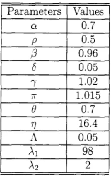
Table 1 shows the values of the parameters used to simulate the models. Some of these parameters we keep fixed for all simulatiollS since they do not change the basic results. Every time we change a parameter it ,viH be noted. Therefore, unless otherwise stated, the parameters of Table 5.1 are used.
The relative price of good z changes over time. \Ve will use the price of
one period to compute real GDP. The real GDP in period t is
GDPt
=
Xt' PoThat is, real GDP is measured in prices of period zero. Further, since the
population is constant the growth rate of real GDP and of real GDP per capita are the same.
To compute the grO\vth rate of GDP we will follow the procedure of the
US government's Bureau of Economic Analysis. For t
2::
2, we calculate thegrowth rate of GDP in period t, gt, in the following way:
where Xt
=
(Yt, Zt) and Pt=
(l,pzd·A little bit more about notation should be said. After each variable we
the Free Trade economy or the Quota Economy, respectively. For example,
GDPf(t) is the value of the GDP in the Free Trade Economy in period t.
Now, let us analyze one of the results listed in the beginning of this
sec-tion19:
1) GDP is greater in the free trade economy than in the quota economy.
Further for some parameter values this difference is a factor of thirty:
Looking at Table 2 we see that real GDP of the free trade economy is
higher than real GDP of the quota economy for any value of A
>
1. Thereason for this persistent difference between GDP in both economies is as
follows. vVith a quota there is alv"ays a group of workers using an old
tech-nology (a smaller TFP). This group ohvorkers has smaller productivity and, consequently, a smaller capital-labor ratio. As a result the quota economy has a smaller capital-labor ratio and a smaller TFP than the free trade econ-omy. These two fadors together explain the difference of GDP between the free trade and the quota economy.
Parente and Prescott
[?J
and Chari, McGrattan and Kehoe[?J
using asample of countries calculated the difference of income per capita between
the richest and the poorest countries. In both papers this difference is around
30 times.20
As we see in Table 2, the GDP per capita of the free trade economy
com-pared with the quota economy is on average more than 30 times for A
>
1.But, this difference is sensitive to the amount of protection that the z sector
receives. In other words, the difference is sensitive to the value of A. \Ve
compute the average value of the ratio of GDP in the free trade economy to the GDP in the quota economy for different values of A. As we can see if
A
=
1 than we get this difference to be equal to the values found by Parenteand Prescott
[?J
and Chari, セvi」gイ。エエ。ョ@ and Kehoe[?J.
Now let us look atthe second result listed above.
19The tables and graphs of the other results are available by request.It also can be seen in Teixeira r?].
5
Conclusions
\-Ve started this paper asking why the technologicallevel differs over time and across countries. In this paper we answered this question using international trade and the institutional arrangements.
The importance of the institutional arrangements comes from their ca-pacity to control groups that otherwise would block the adoption of new technologies. On the other hand, international trade (the free trade arrange-ment or the tariff arrangearrange-ment) guarantees that any firm, producing in any country, will use the best technology available in the world. \Vith quota there is resistance to adopt new technologies and firms generally wiU not use the most productive technology available.
The intuition behind these results is the foUowing. First, with free trade the prices are determined in the international markets and firrns are in com-petition with the productivity leaders. Skilled labor then does not resist the adoption of new technologies because given the price of its product, produc-ing most effi.ciently maximizes its income and its utility. Under a tariff, the domestic price equals the international price times a constant factor (one plus
tariff). It does not break the link between the domestic and international
price and so the same argurnent as under free trade applies.21 In contrast,
if a quota is introduced then the domestic price becomes independent of the international price. In this case, skilled labor can increase the relative price of the good produced in its sector by blocking the use of a new technology. This can increase the income of skilled labor and so be in its interest to resist new technologies. This is the case if technological progress is not too rapid
(small r) and skilled labor is a relatively small group that faces a relatively
large internaI market. The intuition is that on one hand, if the technology advances too rapid then the opportunity cost of not using the most advanced technology is too large. On the other hand, if the domestic market is rel-atively small, then the gain from manipulating the domestic price is not suffi.cient relative to the cost.
In our model the difference in productivity between the free trade econ-omy and the quota econecon-omy is not explained by the difference in the capital-labor ratio; instead the difference in the capital-capital-labor ratio are caused by differences in total factor productivity. The use of old technologies (a smaller TFP) reduces the productivity of capital. With a lower productivity there
is less investment and a smaller capital stock. A smaller capital stock \vith
smaller TFP explains the smaller labor productivity. Furthermore, a smaller
capital stock used with an old and less productive technology explains the difference in the GDP between the free trade and the quota economy.
A poor country is one where workers have smaller productivity and hence a smaller in come per capita. In this paper countries are poor (and save less) because they do not use the best technologies available. The reason countries use different technologies is that their internaI arrangements allow groups to resist adoption of new technologies. In other words, countries are poor not because they have smaUer capital labor ratio, but they have smaller capital labor ratio because they are poor.
In this mode!' there exists no open poor economies. A poor country that opens itself to international trade would grmv faster than the other economies catching up, eliminating all differences in the income per capita.
Closed economies, on the other hand. could be richer than a free trade economy, which would depend on the internaI institutional arrangements.
If the internaI institutional arrangements were able to control groups that
otherwise would resist new technologies, then a country would not depend on international trade to keep technological progress (see Proposition 5). :vloreover, with quota and no blocking, this economy can have a higher GDP than the free trade economy. Once the market is closed investment jumps. This has a permanent effect on the capital stock. Consequently it has a permanent effect on production of the protected sector and on GDP. In this case, a quota has a leveI effect in GDP. This leveI effect increases the grmvth rate of the economy during the transition. But, as we saw before, with quota and if groups can resist new technologies the same technology wiU be used for a longer period than in the free trade economy. As a consequence of this lack of technological progress, the quota economy gets a smaller TFP, reducing the productivity of capital that reduces investment and GDP.
•
closed countries growing at low rates.
For future research adopting the approach used in this paper there are some constraints that we could relaxo One constraint is about population grO\vth. This could be easily introduced into the model if all groups have the same grov,rth rate. In this case, the growth rate of the GDP would increase by the value of the grO\vth rate of population. The grO\vth rate of GDP per
capita would not change. If \ve assume different grov.rth rates for groups then
\ve could have some different results. For example, if the type 2 group grows faster than the other groups the proportion of type 2 in the population would increase over time. In this case, the ty-pe 2 coalition would end in a finite number of periods.
Another constraint that we could relax, and maybe a more interesting one, is the movement of capital across and inside the country. \Vhat v;ould
happen in this model if capital could move across countries? :vly intuition
Table 1: Parameters
Parameters Values
o: 0.7
p 0.5
i3
0.966 0.05
í 1.02
TI 1.015
e
0.7TJ 16.4
l\. 0.05
),1 98
),2 2
Table 2: GDPfjGDPq for Different LeveIs of Protection
A Average GDPf(t)jGDPq(t)
0.05 98.1
0.5 45.5
1 28.7
1.5 19.8
"
セセ@ "\ '..1' L' " '
j
.'," '.
GセセGI@ セL@
c·
,,:
#'
⦅BBLLLMLLLLBBMセセ@ .. _.çJ
-
"',,,
\FUNDAÇÃO GETULIO VARGAS
BIBLIOTECA
l エNNLtセ@ "'(11, I GセNセヲM ['r .r >f セャャ@ t • fi. セ@ !'i I, Jít, ,i.
セja@ II[ r I/,IA [.,\ r A ',1.\[': N .\
'\.Cham. P/EPGE SPE tセVHゥエ@
Autor TeIxeira. Arilton
Título Effccts oftrade poliey on teehnology adoption and