Spatial product partition model through spanning trees

SPATIAL PRODUCT PARTITION MODEL THROUGH

LEONARDO VILELA TEIXEIRA

SPATIAL PRODUCT PARTITION MODEL THROUGH

SPANNING TREES

Dissertation presented to the Graduate Program in Computer Science of the Fed-eral University of Minas Gerais in partial fulfillment of the requirements for the de-gree of Master in Computer Science.

Advisor: Renato Martins Assunção

Co-Advisor: Rosangela Helena Loschi

LEONARDO VILELA TEIXEIRA

MODELO PARTIÇÃO PRODUTO ESPACIAL

USANDO ÁRVORES GERADORAS

Dissertação apresentada ao Programa de Pós-Graduação em Ciência da Com-putação do Instituto de Ciências Exatas da Universidade Federal de Minas Gerais como requisito parcial para a obtenção do grau de Mestre em Ciência da Com-putação.

Orientador: Renato Martins Assunção

Coorientador: Rosangela Helena Loschi

© 2015,Leonardo Vilela Teixeira. Todos os direitos reservados.

Teixeira, Leonardo Vilela.

T266s Spatial Product Partition Model through Spanning Trees / Leonardo Vilela Teixeira. — Belo Horizonte, 2015.

xxvi, 72 f. : il. ; 29cm

Dissertação (Mestrado) — Universidade Federal de Minas Gerais – Departamento de Ciência da

Computação.

Orientador: Renato Martins Assunção:

1. Computação Teses. 2. Classificação espacial -Teses. 3. Teoria bayesiana de decisão estatística – Teses. 4. Variáveis latentes – Teses. I Orientador II. Título.

Acknowledgments

I could not have completed this work without the help and support of many people throughout these years.

I want to thank my family for their continuous support and encouragement. My parents are a constant source of inspiration, always showing me how to be a better person. To my beloved sister, even though the distance has made our physical reunion less frequent, thank you for being always there for me. To my little niece, your arrival has been a constant source of joy in our lives.

To my advisor, Prof. Renato Assunção, thank you for being a real mentor and for your guidance in the past couple of years. You’ve done much for me and I con-stantly learn from you. I also thank my co-advisor, Prof. Rosangela Loschi, who has become a joyful presence on our weekly meeting, and whose contributions were es-sential to keep this work on the right tracks. To all the professors who contributed to my professional growth, thank you for your valuable lessons. To the secretaries who work at the DCC, thank you for being always so helpful.

I also thank all my friends, who constantly make my life happier. To my univer-sity colleagues, who shared the joy and challenges of these past years, thank you. To my gaming friends who transformed many afternoons and nights into delightful and entertaining moments of racing camels, eating bamboo and building settlements, I say this: you are the best! Lastly, to the group of friends, who are the brothers with whom I don’t share blood, I thank each of you twenty six times!

Finally, I wish to thank you, who is reading this work. Thank you for devoting your time to check this, which has been an important part of my life. I hope you find it useful.

“Das Auge sieht weit, der Verstand noch weiter” (German proverb)

Resumo

Ao analisar dados espaciais, muitas vezes há a necessidade de agregar áreas geográficas em regiões maiores, um processo chamado de regionalização ou agru-pamento com restrições espaciais. Este tipo de agregação pode ser útil para tornar a análise de dados tratável, reduzir o efeito de diferentes populações levando a uma melhor manipulação estatística dos dados ou até mesmo para facilitar a visualização. Neste trabalho, apresentamos um novo método de regionalização que incor-pora o conceito de árvores geradoras a um modelo estatístico, formando um novo tipo de modelo partição produto espacial. Ao condicionar as partições em quebras de árvores geradoras, reduz-se o espaço de busca, possibilitando a construção de um algoritmo eficaz para amostragem da distribuição a posteriori das partições.

Nós mostramos que, ao usar um modelo estatístico Bayesiano, é possível aco-modar melhor a variação natural dos dados e diminuir o efeito de valores extremos, produzindo assim melhores resultados quando comparado com as abordagens tradi-cionais. Nós também mostramos como nosso modelo é flexível o suficiente para acomodar dados com diferentes distribuições. Finalmente, nós avaliamos o nosso método através de experimentos com dados simulados, bem como através de dois estudos de caso.

Palavras-chave: classificação espacial; modelos de partição; modelos latentes; apren-dizagem bayesiana de estrutura.

Abstract

When performing analysis of spatial data, there is often the need to aggregate geographical areas into larger regions, a process called regionalization or spatially constrained clustering. This type of aggregation can be useful to make data analysis tractable, reduce the effect of different populations for a better statistical handling of the data or even to facilitate the visualization.

In this work we present a new regionalization method which incorporates the concept of spanning trees into a statistical framework, forming a new type of spatial product partition model. By conditioning the partitions to splits of spanning trees we reduce the search space and enable the construction of an effective sampling al-gorithm.

We show how using a Bayesian statistical framework we are able to better ac-commodate the natural variation of the data and to diminish the effect of outliers, producing better results when compared with the traditional approaches. We also show how our model is flexible enough to accommodate distinct distributions of data. Finally, we evaluate our method through experiments with simulated data as well as with two distinct case studies.

Palavras-chave: spatial clustering; partition models; latent models; Bayesian struc-ture learning;.

List of Figures

1.1 Example of regionalization . . . 2

1.2 Example of a bad regionalization . . . 4

2.1 Illustration of different graph types . . . 11

2.2 Example of the model for the data as a graph . . . 13

3.1 Example of a spanning tree . . . 24

3.2 Groups generated by spanning tree process . . . 25

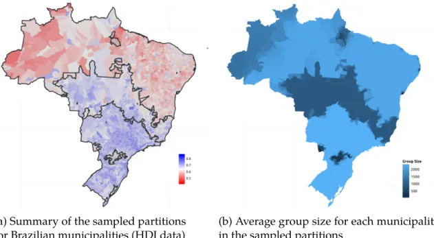
6.1 Map of municipalities of Brazil with HDI data . . . 58

6.2 Regionalization of Brazilian municipalities according to their HDI . . . . 58

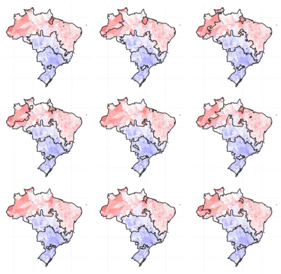
6.3 Some of the sampled partitions (HDI data) . . . 59

6.4 Ratio between the actual and expected number of deaths by cancer . . . 61

6.5 Summary of the regionalization (Cancer deaths) . . . 61

6.6 Other regionalization methods results for the lung cancer map . . . 62

6.7 Other regionalization methods results for the bladder cancer map . . . . 63

6.8 Average size of the clusters (cancer deaths) . . . 63

6.9 Some of the sampled partitions (lung cancer) . . . 64

6.10 Some of the sampled partitions (bladder cancer) . . . 64

List of Tables

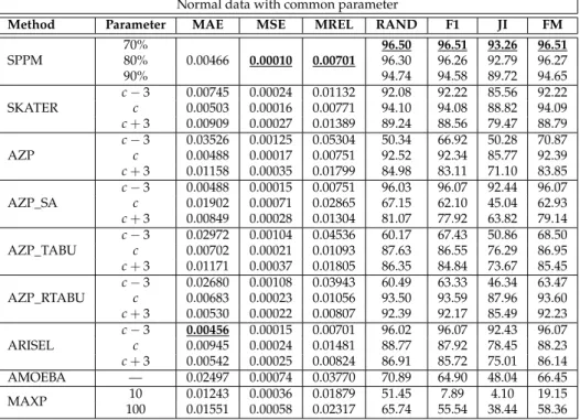
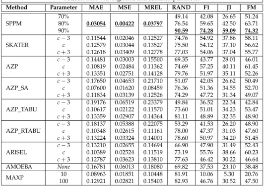
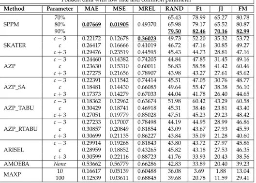
6.1 Model Fit, Normal data with common parameters . . . 54

6.2 Model Fit, Normal data with distinct parameters . . . 54

6.3 Model Fit, Poisson data with high rate and common parameters . . . 55

6.4 Model Fit, Poisson data with high rate and distinct parameters . . . 55

6.5 Model Fit, Poisson data with low rate and common parameters . . . 56

6.6 Model Fit, Poisson data with low rate and distinct parameters . . . 56

List of Algorithms

1 The Metropolis-Hastings algorithm. . . 15 2 Sampling a uniform tree given a partition . . . 29 3 Sampling the tree using MST algorithm . . . 30

List of Abbreviations

HDI Human Development Index

IBGE Instituto Brasileiro de Geografia e Estatística

IPEA Instituto de Pesquisa Econômica Aplicada

MCMC Markov Chain Monte Carlo

MRF Markov Random Field

PPM Product Partition Model

SPPM Spatial Product Partition Model

UNDP United Nations Development Programme

Contents

Acknowledgments ix

Resumo xiii

Abstract xv

List of Figures xvii

List of Tables xix

List of Algorithms xxi

List of Abbreviations xxiii

1 Introduction 1

1.1 Motivation . . . 1 1.2 Contributions . . . 4 1.3 Outline . . . 4

2 Background and Theoretical Framework 7

2.1 A description of the problem. . . 8 2.1.1 Clustering . . . 8 2.1.2 Spatially Constrained Clustering . . . 9 2.2 A graph representation . . . 10 2.2.1 Basic definitions . . . 10 2.2.2 The modeling of the data using graphs. . . 12 2.2.3 The task in terms of the modeling. . . 12 2.3 Markov Chain Monte Carlo Methods . . . 14 2.3.1 Metropolis-Hastings algorithm . . . 14 2.3.2 Gibbs sampler . . . 16

2.4 Product Partition Model . . . 17 2.5 Related Work. . . 19

3 Sampling partitions using Spanning Trees 23 3.1 Using a spanning tree to explore the partitions . . . 23 3.2 Sampling partitions and tree . . . 25 3.2.1 Generic model for sampling partitions . . . 26 3.2.2 Gibbs sampler for the partition . . . 27 3.2.3 Sampling the tree . . . 28

4 Spatial PPM induced by spanning trees 31

4.1 Proposed model . . . 31 4.2 Gibbs sampler for the SPPM . . . 34 4.3 SPPM for Normal data . . . 36 4.4 SPPM for Poisson data . . . 37

5 MRF-SPPM 39

5.1 The model . . . 39 5.2 Proposed modifications. . . 43 5.3 Shortcomings of the model. . . 44

6 Experimental evaluation 47

6.1 Simulations. . . 47 6.1.1 Evaluation metrics . . . 49 6.1.2 Methods used in the comparison . . . 52 6.1.3 Results . . . 52 6.2 Applications . . . 57 6.2.1 Normal data: HDI. . . 57 6.2.2 Poisson data: Cancer deaths . . . 60

7 Conclusion 65

Bibliography 67

Chapter 1

Introduction

1.1

Motivation

We collect, represent, and store data in an effort to better understand our world and to help us make decisions. Once we have the data, the study and analysis of it becomes a central and important activity.

In many situations there are spatial characteristics naturally associated with the data. Human beings, for instance, are neither uniformly nor arbitrarily distributed in space. Frequently, geographical characteristic such as topology, weather, and oth-ers may affect the behavior and the spatial distribution of individuals. The recent advances in science and technology have made the acquisition and usage of spatial data not only something easier but also a more present task. Therefore, the spatial analysis becomes a particularly important exploratory and analytical tool.

When performing spatial analysis, it is often needed to aggregate geographi-cal areas into larger regions. This can serve a range of purposes, such as reducing the noise introduced by outliers and inaccurate data, make data analysis tractable, providing a better statistical handling of the data (by reducing the effect of different populations), and even simply to facilitate the visualization and understanding of the information [Wise et al.,1997].

There are two possible ways to carry out this aggregation. One way is through an artificial aggregation, where the constructed regions are defined rather arbitrarily or using official or normative designations (such as states, districts and counties). This kind of aggregation, however, is usually the expression of political will and may not take into account the geographical characteristics or information specific to the domain being studied. Another way is to perform the aggregation based on the analysis of characteristics of data which are related to the phenomena being studied.

2 Chapter1. Introduction

Through the use of official or nominative regions, in many cases, the result of statistical analysis can be affected by problems of the aggregation, such as the eco-logical fallacy [Robinson, 1950; Openshaw, 1984a], the modifiable areal unit prob-lem [Openshaw,1984b], among others. Therefore, the use of analytical regions is of particular relevance since this kind of analysis, if properly executed, may be able to produce more helpful results in the discovery of spatial patterns than the original data [Alvanides and Openshaw,1999].

In spatial analysis, this type of aggregation receives the name ofregionalization orspatially constrained clustering. It is the process of aggregating small contiguous geographical areas forming larger regions (called spatial clusters), with the purpose of partitioning the space into spatial clusters in a form such that areas which are sim-ilar according to some characteristics belong to the same spatial cluster. InFig. 1.1 we show an example of an outcome of a regionalization method. The3127 conti-nental US counties have been aggregated into seven regions or clusters according to their percentage of votes for George Bush in the US Presidential Election of 2004. Neighboring counties with similar voting percentages are clustered together.

Figure 1.1: Example of regionalization as seen inGuo[2008]

1.1. Motivation 3

VAregional system determined service areas boundaries taking into account the ex-pected patterns of health service use [Ricketts,1997]. Other examples of applications are: sampling procedures [Martin,1998], establishment of communication protocols in geo-sensor networks [Reis et al.,2007], classification of areas with high incidence of diseases [Martins-Bedé et al., 2009], and environmental planning [Bernetti et al.,

2011].

Most of the regionalization techniques consider the data as fixed, static values. Frequently, this assumption is inappropriate, as it doesn’t allow for measurement er-ror or uncertainty on the areas’ measures and it doesn’t allow also for the evaluation of the uncertainty of the obtained clusters. It is valid to think of neighbouring areas as having similar values due to an underlying process which has a regional effect. Or to consider the collected data as only a random manifestation of some characteristic which may vary in time.

Consider, as an example, the measured infant mortality rate of a small town in a given year. This value should not be considered as the most representative value for the true mortality rate. This value can be severely impacted by small differences from one year to another, particularly if the area has a small population. The mea-sured value can show a natural variability, expressed in this widely different infant mortality rate variation in two successive years in small population areas, which is not considered in the traditional regionalization techniques. Thus, using a explicitly stochastic framework to perform the regionalization can provide better and more helpful results. InFig. 1.2a regionalization produced by a non-stochastic method is shown. This is a map of municipalities in the South of Brazil partitioned according to their value of the bladder cancer mortality rate. The regionalization technique used is named Automated Zoning Procedure.

4 Chapter1. Introduction

Figure 1.2: Example of a bad regionalization

1.2

Contributions

In this work we incorporate the concept of spanning trees into a hierarchical Bayesian model, introducing a new spatial product partition model. Our model al-lows for any type of distribution for the observed data.

By conditioning the partitions to splits of spanning trees, we substantially re-duce the space of partitions or clusters we have to explore. The clustering struc-ture assumes a product form, which conveniently allows for some sort of conjugacy where the posterior distribution can be derived from the prior distribution of each cluster. Based on this framework, we propose an efficient Gibbs sampler algorithm to sample from the posterior distributions, specially that of the partition.

Through our new model, we provide a new framework to cluster data which is flexible and can be used to model data with different structures, and yet effective and viable for inference to be made through a Gibbs sampler. Examples of application of the proposed model and the sampling algorithm are provided for data modelled through Normal and Poisson distributions.

1.3

Outline

re-1.3. Outline 5

Chapter 2

Background and Theoretical

Framework

The goal of this chapter is to introduce the elements needed to understand both the problem we have at hand as well as the proposed solution. We also take a mo-ment to review previous literature that is related to the problem and the main current solutions to it.

Throughout this text, we attempt to maintain a consistent notation. We use bold font to denote vectors of random variables and Greek letters to denote parameters in a model. We denote the data vector byY _{= (Y1,· · · ,Yn). Hyperparameters and} indices are denoted by lower case letters. A partition of a set of indices is denoted by the Greek letterπand T represents a spanning tree. Gkdenotes the k-th cluster (or

the subgraph induced by the nodes in the groupGkwhen talking about graphs). We

use f(·)and f(· | ·)to denote marginal and conditional probability density function as well as probability mass function when in the continuous and discrete random vector case, respectively.

We start with Section 2.1, in which we give a textual description of the prob-lem and the task we seek to solve in this work. This description builds upon what was already stated in the introduction and forms the base for the model we describe next. InSection 2.2, a formulation of the problem in terms of a graph is given. Such a modeling is helpful to understand the nature of the data and is an opportunity to define and explain in more detail the elements involved in both the problem as well as the proposed solutions. Next, in Section 2.3, a brief overview of some Markov Chain Monte Carlo (MCMC) sampling techniques is presented, to help those unfa-miliar with such tools to follow the next chapters. Finally, inSection 2.5we provide a review of the literature and the work that are related with our problem.

8 Chapter2. Background and Theoretical Framework

2.1

A description of the problem

2.1.1

Clustering

Cluster analysis (or simplyclustering) is one of the main tasks in unsupervised machine learning. The goal of clustering is to partition a set of objects into groups (calledclusters) in such a way that the objects of a given cluster are similar to each other and differ from the objects of other clusters.

Tasks or problems involving clustering are not recent, with examples that go back decades in disciplines as psychology, geology, marketing, and many other fields [Zubin,1938;Tryon,1939;Cattell,1943]. The problem is also generic enough, with so many different assumptions and constraints, that several different approaches have emerged over the years.

Generally, the process of clustering consists of partitioning a set of n objects, each object withkfeatures (or attributes). To define the clusters, asimilarity measureis usually necessary, to indicate how similar are two objects. Frequently, this measure is some kind of distance measurebetween the objects, such as the Euclidean distance between numeric vector objects.

There are many variations on the clustering problem, due to the varied num-ber of assumptions and constraints that take place. As a result, many algorithms with different approaches have been developed over the years. These different ap-proaches can usually be divided into two categories: hierarchical and partitional methods. The hierarchical methods generate a nested series of partitions, while the partitional methods generate only one. This taxonomy can be further extended with descriptions such as: connectivity based (builds on the idea that objects are more similar to nearby objects than to farther objects), centroid based (represent the clus-ters through centroids - a mean vector), density based (define cluster by the density of the data nearby each object), graph based (work upon connectivity definitions in graphs), fuzzy clustering (each object belongs to each cluster to a certain degree), distribution models (model the clusters with statistical distributions), among others. Another important type of clustering is the constrained clustering, which is di-rectly connected to the problem which is the main focus of this work. In this kind of clustering constraints are imposed on how the objects can or cannot be grouped together. Usually these constraints impose that two objects must (or cannot) be in the same group. An example is the constrained k-means clustering [Wagstaff et al.,

2001].

2.1. A description of the problem 9

the different types of clustering techniques are discussed but also other related top-ics such as pattern representation, feature selection, similarity measures and appli-cations.

2.1.2

Spatially Constrained Clustering

A particular type of clustering is thespatially constrained clustering, also known asregionalization. In this problem, not only the similarity between the objects is taken into consideration, but also their spatial organization plays an important role on how the clustering process is done.

A typical scenario for this problem is when the data being clustered has its spa-tial characteristic derived from geographic properties. An example is a map divided into small areas. In this case, the goal is to group these small areas into larger regions, according to their similarity.

The main difference with respect to the usual clustering problem is that there is an additional constraint: while the objects are still clustered based on the simi-larity between themselves, the clusters formed must be spatially contiguous. The contiguity, in our example, is defined by the geographic neighbourhood.

It is important to highlight that with spatially constrained clustering we have two distinct spaces. There is a feature space, defined by the values and characteristics associated with the data, which are used to determine the similarity between objects. There is also the constraint space, defined by the spatial relationship present in the data, which restricts how the objects can be grouped together but is not directly used to compute similarity between them. This distinction is important because two very similar objects according to the feature space would be assigned to the same cluster in traditional clustering methods, but may end up in different clusters when the spatial constrain is taken into consideration.

A review of this problem can be found in the survey fromDuque et al.[2007]. In this survey, the authors discuss many contributions to the area in the past decades and also provide a taxonomy of methods for solving regionalization problems. There are two main categories of methods: those that treat the spatial constraints implicitly and those which explicitly incorporate the constraints.

10 Chapter2. Background and Theoretical Framework

regions, still without taking into account the spatial constraints. Weaver and Hess

[1963] published one of the pioneer works in this subject, which proposes a proce-dure to generate political districts.Hess et al.[1965] formally presented this method. In the second category, the methods explicitly consider the spatial constraints and usually model this problem as optimization problems, such as integer program-ming. Search for an exact answer to regionalization through an optimization prob-lem is not computationally feasible [Altman,1998]. Many attempts were made with different formulations of the problem as an optimization problem [Macmillan and Pierce,1994;Garfinkel and Nemhauser,1970;Mehrotra et al.,1998;Zoltners,1979].

Since obtaining the exact solution is unfeasible, different heuristics were pro-posed such as starting regions from a (seed) area and grow them by adding neigh-bouring areas [Vickrey, 1961; Taylor, 1973; Openshaw, 1977a,b; Rossiter and John-ston, 1981] or start from an initially feasible solution and search for improve-ments [Nagel,1965;Openshaw,1977a,1978;Browdy,1990].

2.2

A graph representation

The modeling in terms of a graph becomes quite natural to handle this prob-lem. There is a collection of objects which we want to cluster. There is one or more attributes associated with each of these objects. They also relate to each other in terms of a neighbourhood structure, which gives a constraint on how these objects can be grouped with each other. Our goal is to cluster the objects into groups such that the objects in a group are similar to each other whereas objects from different groups are dissimilar to each other.

The spatial constraint comes into play as we might have two objects which are very similar to each other, but are located on widely separated regions on the map and as such must not be grouped together in the same cluster.

2.2.1

Basic definitions

2.2. A graph representation 11 1 2 3 4 5

(a) A directed graph

1

2

3 4

5

(b) An undirected graph

1

2

3 4

5

(c) A tree

Figure 2.1: Illustration of different graph types

to v, then v is also adjacent tou. Since the graphs we use in this documents are all undirected, we will refer to them simply asgraphs, without using the wordundirected. Apath in a graph is an alternating sequence of vertices and edges, beginning and ending with a vertex, such that all edges and vertices are distinct (with the pos-sible exception of the first and last vertices) and each edge is incident with both the vertex immediately preceding it as well as the vertex immediately following it. A cycle is a closed path, i.e. a path whose first vertex is the same as the last. We say that two vertices areconnectedif there is a path between them. A graph is connected if every pair of vertices of this graph is connected.

Atreeis a undirected connected graph without cycles. In a tree, any two ver-tices can be connected by a unique path. InFig. 2.1these different types of graph are illustrated.

A connected component (or just component) of an undirected graph G is a connected subgraph of G which is not contained in any connected subgraph of G

with more vertices or edges than it has. In other words, if we grow the subgraph by adding vertices or edges of Gthat are not currently in it, the subgraph becomes disconnected. There is no vertex outside of the subgraph that can be connected to a vertex of the subgraph;

It is also possible for each edge of a graph to have aweightw_ij associated with it, in which case we call the graph a weighted graph. The number of nodesis given by |V| =nand we denote byu ∼vthe adjacency relation between verticesuandv.

Aspanning treeof a graph G is a tree thatspansG. That is, it is a tree that has all the nodes of G and some of the edges of G. In other words, a spanning tree of

12 Chapter2. Background and Theoretical Framework

forest- a set of trees, each of them a spanning tree for one of the components of the graph.

2.2.2

The modeling of the data using graphs

The data is modeled in the following way: the objects (which represent ran-dom variables, ranran-dom vectors or other data associated with each location) are rep-resented by vertices, so for each object we have a vertex. The neighbourhood struc-ture is modeled through the edges. That is, each edge(u,v)represents that nodesu

andv are adjacent. This model is quite natural and is basically a translation of the data into a graph. The geographical neighbourhood structure in the data is mapped to the neighborhood in the graph.

As an example, inFig. 2.2we show the map of Belo Horizonte city, divided into its administrative regions. The resulting graph built from this map is superimposed in the figure.

Formally, we describe the model such as:

• The graph G = (V,E) is built withV being the set of nodes vi where each vi

represents an object (data point).

• The edge set E ={(u,v) ∈ V×V | adj(u,v)}where each edge represents the adjacency between two objects.

• Each vertex has a set of (one or more) attributes, which are the data associated with each object in the dataset. Thus, for each vertex v_i, we represent its at-tributes asY_{i. These attributes can be a vector of attributes, a single attribute} or can even be a set of features and a response variable.

2.2.3

The task in terms of the modeling

Considering the model we described, the task at our hands of clustering the data into groups where the spatial constraint is respected (i.e. groups where each object is adjacent to another object of the group) can be translated into the task of partitioning the graph.

In a more formal way, what we want is to partition the set of verticesV intoc

distinct groups,Gk,k =1,· · · ,c, such thatV =Sck=1GkandGi∩ Gj=∅,∀i 6= j.

To ensure the spatial constraint, we also assume that

2.2. A graph representation 13

Figure 2.2: Example of the model as a graph for the administrative regions of Belo Horizonte

Another way to describe this constraint is to say that each groupGk is a

con-nected subgraph. If we remove from the original graph all the edges connecting nodes from different groups, the resulting graph will be a disconnected graph and for each of its connected components, the set of its nodes is exactly one of the groups defined by the partitioning.

14 Chapter2. Background and Theoretical Framework

whereas vertices from different groups have dissimilar attributes.

The definition of what is meant by similar and dissimilar is not given here and it is usually one of the points where the algorithms to solve this problem differ. When we discuss the modeling of our proposed solutions (and the related works) this con-cept of similarity will become more clear.

2.3

Markov Chain Monte Carlo Methods

One important class of tools used in our solutions is the Markov Chain Monte Carlo (MCMC) methods. These algorithms for sampling from a probability distri-bution are based on the construction of an appropriate Markov chain.

The general idea behind MCMC methods is that we want to sample from a given probability distribution f(x)which is complex and from which we don’t know how to sample directly. The way these methods work is by constructing a Markov chain in a specific way such that thestationary distributionof the chain is the desired probability f(x)from which we want to sample. The samples are taken, therefore, by carrying out a random walk on the constructed chain.

In this section we briefly describe the two main MCMC methods, namely the Metropolis-Hastings algorithm and the Gibbs sampler, which we used in our work. More information about these methods can be found in various sources, such as in the introductory paper byAndrieu et al.[2003] or in the book byMurphy[2012].

2.3.1

Metropolis-Hastings algorithm

This algorithm, initially proposed byMetropolis et al.[1953] and later extended to a more general case byHastings [1970] presents a way of sampling from a target distributionP(x)(possibly multivariate) from which we can’t directly sample. This distribution might be too complex, or it may be even not completely specified (i.e. it can be specified up to a normalizing constant).

2.3. Markov Chain Monte Carlo Methods 15

Asit was said, the algorithm is based on the construction of a Markov chain in such a way that the stationary distribution is exactly the target distributionP(x). To achieve such a distribution, some conditions must be met. The chain must beergodic (i.e. irreducible, aperiodic and positive recurrent) to guarantee the uniqueness of the stationary distribution. The detailed balance is used as sufficient condition to make sure such stationary distribution will exist. The acceptance rule mentioned in the previous paragraph is defined to ensure these conditions are attained. The accep-tance ratio, which is used to determine if the new candidate x′ should be accepted or rejected in the Metropolis-Hasting algorithm, is given by

A(x(t−1) →x′) =min 1, P(x′)

P(x(t−1)₎

Q(x′ →x(t−1))

Q(x(t−1) _→x′₎

!

, (2.3.1)

where Q(x → y) denotes the probability of the proposal distribution, that is, the probability of proposing the stateygiven the statex.

At each step of the process, a new candidate is sampled. Then, this acceptance ratio is computed. Finally, a uniform value between 0 and 1 is sampled and com-pared with the acceptance ratio to decide if the new candidate should be accepted or rejected. InAlgorithm 1, the pseudo code for the Metropolis-Hastings algorithm can be seen.

Algorithm 1The Metropolis-Hastings algorithm 1: procedureMetropolis-Hastings

2: x(0) ←random initial value 3: fort←1,N do

4: x′ ←sample fromQ(x_|x(t−1)) 5: A(x(t−1) →x′) =min1, P(x′)

P(x(t−1)₎

Q(x′→x(t−1)₎

Q(x(t−1)_→x′₎

6: u←U(0, 1)

7: ifu≤ A(x(t−1) →x′)then 8: x(t) ←x′

9: else

10: x(t) ←x(t−1)

11: end if 12: end for 13: end procedure

16 Chapter2. Background and Theoretical Framework

that, in the acceptance ratio, both directions in the proposal distribution are needed (i.e. we need both Q(x′ _→ x(t−1)) and Q(x(t−1) _→ x′)). It is also worth to note that in the case of these two values being the same (i.e. the distribution is symmet-ric), the algorithm becomes the simpler Metropolis algorithm, where the proposal distribution density is not needed to compute the acceptance ratio.

2.3.2

Gibbs sampler

Gibbs sampler (or Gibbs sampling) was introduced by Geman and Geman

[1984] and named after the physicist Josiah Willard Gibbs, in reference to an anal-ogy between the sampling algorithm and statistical physics. It is a special case, in its basic incarnation, of the Metropolis-Hastings algorithm.

The Gibbs sampler is particularly useful when the probability from which we want to sample is multivariate and it is unknown or difficult to sample from it, whereas the full conditional distribution of each variable is known and easy to sam-ple from.

The Gibbs sampler provides a way for sampling from the distributionP(x_)by sampling each of its componentsx_i at a time, from the full conditional distribution. Suppose we want to obtain a sample from a joint distribution f(x1,· · · ,xn).

The i-th sample is denoted by X(i) _{= (x}(i)

1 ,· · · ,x

(i)

n ). The algorithm proceeds as

follows:

• Start with some initial stateX(0)_.

• For the i-th sample, sample each dimension j = i,· · · ,n from the full condi-tional distribution:

P(xj | x(₁i),· · · ,x(_j−i)₁,x(_j+i−11),· · · ,x

(i−1)

n ). (2.3.2)

It is important to note that we always use the most recently sampled value for each variable and update the value of a variable as soon as a new value is sampled.

The Gibbs sampler is a special case of the Metropolis-Hastings algorithm. Take the proposal distribution as that inEq. (2.3.2). Then, the Metropolis-Hastings ratio inEq. (2.3.1) is equal to1and the acceptance rate is also1. That is, every sample is accepted.

2.4. Product Partition Model 17

Gibbs sampler, in which two or more variables are grouped together and sampled from their joint distribution conditioned on all other variables. Another one is the collapsed Gibbs samplerwhich integrates out (marginalizes over) one or more variables when sampling for some other variable.

2.4

Product Partition Model

In this section we review the product partition model (PPM), introduced by

Barry and Hartigan[1992], which is a convenient framework to model data that

fol-low different regimes.

In the PPM, it is assumed that observations in different components of a ran-dom data partition are independent and those inside a component are independent and identically distributed (iid). Moreover, the probability distribution for the ran-dom partition assumes a product form.

Let Y _{= (Y1,· · · ,Yn) be a set of observed data. Consider a random partition} π={(Y_1,1,· · · ,Y_1,n1),· · · ,(Y_c,1,· · · ,Yc,nc)}of this data intocgroups of contiguous

objects where the k-th group hasn_k observations. Denote byY_G

k = (Yk,1,· · · ,Yk,nk)

the observations in thek-th group.

We say that the random quantity(Y_{,π)follows a PPM, denoted by (}Y_{;π) ∼}

PPMif the following two conditions are met:

(i) The prior distribution of partitionπintocblocks is given by the following prod-uct distribution:

P(π) = L

c

∏

c(Gk), (2.4.1)

wherec(Gk)is a nonnegative number which expresses the similarity among the

observations belonging to groupk, andLis a constant chosen so that the sum ofP(π) over all possible partitions is unity. The component c(Gk) is named

prior cohesion of groupkand is a subjective choice.

(ii) Conditionally on the partitionπ, the sequenceY _{= (Y1,· · · ,Yn)has the joint} density given by:

f(Y _{| π) =}

c

∏

f_Gk(Y

18 Chapter2. Background and Theoretical Framework

where f_Gk(Y

Gk)is the joint density of the random vectorYGk = (Yk,1,· · · ,Yk,nk),

called data factor. That is the block of n_k observations belonging to the k-th group.

A more interesting type of product partition model, which is considered in our work, is a model in which a set of parametersθ₁,· · · ,θnis partitioned intocgroups,

inducing a partition in the dataset. Given a partition, there are common parameters θ_G1,· · · ,θ_Gkof each group that are assumed to be independent. The joint distribution of the parameters, the data and the partition is a product partition model. The joint distribution of the parameters and the data, given a partition can be expressed as:

f(Y_{,θ| π) =}

c

∏

f(Y_G

k|θGk)f(θGk),

where

f(Y

Gk |θGk) =

∏

i∈Gk

f(Y_{i | θ} Gk).

Thus, the joint distribution of the random variables in cluster Gk, that is, the

data factor, becomes:

f(Y Gk) =

Z

Θ "

∏

f(Y_i|θ Gk)

#

f(θ_Gk)dθ_Gk,

the posterior by cluster ofθ_Gk, givenY Gk, is

f(θ_Gk |Y Gk) =

∏_i∈G

k f(Yi | θGk)

f(θ_Gk)

f(Y_G

k)

and consequently, the marginal posterior of each individual parameterθ_ibecomes

P(θ_i | Y_{) =}

∑

k |YGk)P(Gk ∈ π |Y),

where the sum is over all possible partitions andGkis the group that containi. The

posterior distribution for the partition assumes the form

P(π |Y₎ ∝

c

∏

2.5. Related Work 19

and, finally, the posterior distribution for the number of clusters is given by

P(C =c |Y_{) =}

∑

where the sum is over all possible partitions and I[π,c]is an indicator function as-suming1if the partitionπis composed ofcclusters and zero otherwise.

The PPM thus offers a convenient framework to do inference on clustered pa-rameters, since it implies some sort of conjugacy on the model. We explore this in order to perform the inference on both the parameters θ_i as well as in the partitions of the observations.

2.5

Related Work

Many different methods and improvements have been proposed to deal with the problem of regionalization. Openshaw and Wymer[1995] proposed a simulated annealing variant of the k-means with a posterior step to enforce the spatial con-straint. Variants of the Automatic Zoning Procedure(AZP) were proposed using dif-ferent search procedures such assimulated annealing, andtabu search[Openshaw and Rao, 1995]. These methods work as an optimization problem and the number of regions to be constructed must be informed.

A modification of the AZP with tabu search was proposed by Duque and

Church [2004] and is named Automatic Regionalization with Initial Seed Location

(ARiSeL). Under this method, the construction of an initial feasible solution is re-peated several times before running the tabu search. The author argue that con-structing initial solutions is less expensive than performing a local search.

Kohonen[1990] proposed an algorithm calledSelf Organizing Maps(SOM), an

unsupervised neural network which adjust its weights to represent a data set distri-bution on a regular lattice. This method has been used to perform regionalization. However, it doesn’t guarantee the spatial contiguity. A variant of this method is proposed inBação et al.[2004] with a different procedure to explore the neighbour-hood. The same authors proposed a method which uses genetic algorithm to define the center of the regions [Bação et al.,2005].

20 Chapter2. Background and Theoretical Framework

Another technique, calledMax-p-regionsworks by constructing an initial feasi-ble solution and performing local improvement. It clusters the areas into the max-imum number of homogeneous regions such that the value of a spatially extensive regional attribute is above a predefined threshold value [Duque et al.,2012].

Assunção et al. [2006] proposedSpatial ’K’luster Analysis by Tree Edge Removal (SKATER), a graph based method that uses a minimal spanning tree to reduce the search space. The regions are then defined by the removal of edges from the span-ning tree. The removed edges are chosen to minimize a dissimilarity measure.

Inspired by SKATER,Guo [2008] proposed REDCAP (Regionalization with

dy-namically constrained agglomerative clustering and partitioning) with six methods ex-ploring different connection strategies using the underlying graph structure.

There are several statistical methods related to regionalization. In disease map-ping, Knorr-Held and Raßer [2000] presented a Bayesian approach to the spatial partition of small areas into contiguous regions. They assume that each area has a random disease county_iwith Poisson distribution with unknown relative risksθi.

They also assume these relative risks can be grouped intogspatial clusters where the

θi’s have the same value within a cluster. The numbergof clusters is unknown and

hence the unknown parameter vector is composed ofgplus the distinct elements in the vectorθand some additional hyperparameters. Since the parameter vector has a variable dimension, they use reversible jump Markov chain Monte Carlo (MCMC) to obtain a sample from the posterior distribution [Green,1995;Richardson and Green,

1997].

In the same year, Gangnon and Clayton [2000] proposed a different Bayesian approach for this problem. Letr= (r₁,r₂, . . . ,rn)be a specific cluster labelling

func-tion withc clusters. That is, r_i labels the cluster to which area i belongs so r_i = j

wherej =1, . . . ,c. They adopt a prior distributionP(c) ∝ _exp(−∑_jS_j)whereS_j is a known function of thej-th cluster’s geometry,S_j=α+ f(size) +g(shape), which penalizes clusters with large size or convoluted shapes. To make inference on the space of spatial clusters, they propose an algorithm to calculate an approximation to the posterior. This algorithm has two components. The first is a window of plausi-bility, an adaptation of the Occam’s window approach to model selection [Madigan and Raftery,1994]. In the second, given a window of plausibility, they use a random-ized search algorithm similar to backwards elimination methods used for variable selection in regression problems.

Denison and Holmes[2001] also considered this problem. They use a Voronoi

2.5. Related Work 21

search space of the centers is drastically reduced. As inKnorr-Held and Raßer[2000], they also assume that all areas within a tesselation tile have the same distribution de-pending on an unknownθ. They assumea priorithat the probability of a tessellation with Mcenters depends only on the number of centers.

Lu and Carlin[2005] andBanerjee and Gelfand[2006] have worked on a dual

problem: rather than aggregating similar areas into homogeneous regions, they aim to identify sharp boundaries between pairs of areas. Homogeneous regions can be obtained as a byproduct of their procedures. They call their methods boundary (or wombling) analysis.

Hegarty and Barry[2008] proposed a model based on a PPM with cohesions

built in such a way as to take the spatial information into account. While it is an in-teresting Bayesian method, the sampling of the partitions is not simple and a param-eter that indicates whether there will be few or many clusters in the partition must be explicitly and carefully determined since giving it a prior distribution makes the calculations needed for the sampling of the partitions difficult.

Another interesting Bayesian method is proposed byWakefield and Kim[2013]. In the proposed method, the maximum number of clusters has to be specified, the clusters found tend to have a circular shape and the model focus on defining only the clusters which have a "higher" or "lower" value. What means to have a higher or lower value has to be carefully specified through the prior distributions attributed to these two types of clusters.

Chapter 3

Sampling partitions using Spanning

Trees

One of the contributions and main point of this work is the use of a spanning tree as a tool to explore the space of partitions on which we have interest. We start by showing how we can use a spanning tree to simplify the search space of possible partitions. Then, we show how we sample from this space (both trees and partitions). Finally, we describe how this trick is used together with a PPM to make it an effective tool for analysing spatial data.

3.1

Using a spanning tree to explore the partitions

A major problem faced when dealing with partitioning of a dataset or a graph is the huge number of possible partitions that compose the search space. In this section we show how we can use a spanning tree as a tool to tackle this problem and make the exploration of this space of possible partitions something feasible. Back in Chapter 2we showed a graph built for the administrative regions of Belo Horizonte (Fig. 2.2). For that graph, a possible spanning tree is portrayed inFig. 3.1.

The basic idea behind using a spanning tree to generate partitions is that it provides a simple way to get a partition of the dataset conforming to the spatial constraint of having spatially coherent groups.

In a spanning tree, we have a set of n₋1 edges which connect the nodes of the graph. To generate a partition ofcspatially connected groups, the only thing we have to do is to remove c−1edges from this spanning tree. Each edge we remove disconnects a part of the graph, creating a new component (a new group). InFig. 3.2

24 Chapter3. Sampling partitions using Spanning Trees

Figure 3.1: Spanning tree built for the Belo Horizonte data

we show a spanning tree with5groups defined by the removal of4edges (displayed in bold).

3.2. Sampling partitions and tree 25

built from the neighbourhood structure and, therefore, the groups formed will be spatially connected.

Figure 3.2: The groups generated by a spanning tree edge removal and the removed edges

3.2

Sampling partitions and tree

26 Chapter3. Sampling partitions using Spanning Trees

have a connected graphGand we want to sample partitions for this graph.

3.2.1

Generic model for sampling partitions

A simple model for such a situation would be to consider all possible trees and partitions equally probable, that is, the distribution of spanning trees is uniform and the distribution of the partitions, given a specific treeT, is also uniform. So we have the following hierarchical model:

P(T) ∝₁

P(π | T) ∝







1 ifπ ≺ T

0 otherwise,

(3.2.1)

whereπ _{≺ T} means that π is compatible with T, that is, the partition π can be achieved by removing edges from the treeT.

An improvement to this model can be made by changing the distribution of the partitions given a tree. Instead of considering all partitions equally probable, we can model them giving larger probability to those partitions that have a certain amount of groups.

One way of doing that is adding a parameterρ, which models the probability of removing an edge from the tree. In this model, it is as if, for each edge, a coin is tossed, individually, to decide if the edge should be removed or not. The probability of success of this coin isρ. It can be defined as a fixed value or it can be given a prior probability distributions, such as a Beta distribution. This new model becomes:

P(T) ∝₁

P(π| T) ∝







ρ(c−1)(1−ρ)(n−c) ifπ _{≺ T}

0 otherwise.

(3.2.2)

An immediate consequence is that the prior number of clusters is given bynρ. The first model can be seen as a particular case of this new model, where the probability

ρ=0.5.

3.2. Sampling partitions and tree 27

3.2.2

Gibbs sampler for the partition

The Gibbs sampler we describe here is inspired by the transformation sug-gested byBarry and Hartigan[1993]. A partitionπof the graph can be transformed into a vector U _{ofn−1 binary variables, given a compatible spanning tree, where} each variableUirepresents one of the edges of the spanning tree and its value is0if

the edge must be removed from the tree to form πand1otherwise.

With this transformation we can map a partition (given a compatible tree) to a vector U _{and back in a unique way. All possible partitions represent all possible} configurations of this vector. And now, we have a multidimensional random variable which can be sampled with Gibbs sampler. For that purpose, we must be able to specify the full conditional probabilityP(Ui | U−i,T), where we denote byU−ithe

set of all U_j where j ₆= i, that is, U_{−i = {U1,· · · ,Ui−1,Ui+1,· · · ,Un−1}. What is} needed, then, is to decide, for each edge in the tree, given all the other edges, if it should be removed or not. In a general case, it may be hard to specify the exact value of this probability, but since the variable can assume only one of two values, it is sufficient to know the ratio between theP(U_i = 1| U_−i,T)andP(U_i =0 | U_−i,T). We can further develop this

P(U_i =u _|U_{−i,T) =} P(U,T)

P(U −i,T)

= P(Ui =u,U−i | T)P(T)

P(U_−i,T) . so the ratio becomes:

R_i = P(Ui =1| U−i,T)

P(Ui =0| U−i,T)

= P(Ui =1,U−i |T)✟✟ ✟

P(T)✘✘✘✘ ✘✘

P(U_−i,T)

P(Ui =0,U−i |T)✟✟ ✟

P(T)✘✘✘✘ ✘✘

P(U −i,T)

Ri =

P(π(1) | T)

P(π(0) _{| T)},

where π(1) is the partition with the edge U_i and π(0) is the partition without that edge.

28 Chapter3. Sampling partitions using Spanning Trees

U_i =







1 ifR_i ≥ ₁₋u_u

0 otherwise (3.2.3)

In the case of the simple models described above inEq. (3.2.1)and Eq. (3.2.2), this process is simpler and amounts to comparing the uniform valueuto the proba-bilityρand remove the edge ifu ≤ρor leave it in the tree otherwise.

In a more complex model, involving not only the tree and the partition, but also data and parameters, the sampling process is similar. The difference will be seen in the ratio Ri, which must be derived from the model. In this case, the sampling is

done followingEq. (3.2.3).

3.2.3

Sampling the tree

Since we are using a Gibbs sampler, we must also be able to sample a new tree given a partition. The first step for that is to compute the full conditional distribution for the tree, which is given inEq. (3.2.4).

P(T |π = (U₁,· · · ,U_n−1))∝







1 ifπ ≺ T

0 otherwise. (3.2.4)

From that equation, we can notice that the only possible trees to be sampled are those compatible with the current partition - that is, trees from which we can remove edges and get the current partition. These valid trees are uniformly distributed over the subset of trees compatible with the partition.

One way of sampling these trees is by following a hierarchical procedure. First we consider the subgraphs of each group. For each group, we take the subgraph induced by its vertices and sample a uniform spanning tree over this subgraph.

3.2. Sampling partitions and tree 29

Once the new (multi)graph is constructed, we sample a uniform spanning tree for this new graph. The edges selected in this spanning tree are included, together with the spanning trees constructed for each group, in the final spanning tree, which will then be the uniformly selected spanning tree, compatible with the current par-tition.

This procedure can be seen in Algorithm 2. The generation of uniformly dis-tributed spanning trees is a subject of study since 1989 [Broder, 1989]. The main algorithm in the literature (Wilson’s algorithm [Wilson,1996]) is based on a random walk on the graph.

Algorithm 2Sampling a uniform tree given a partition 1: procedureSample-Tree(π,G)

2: G′ ←∅

3: fork←1,cdo

4: Ti ←UniformSpanningTree(Gk)

5: G′ ←Vertex(G_k) 6: end for

7: for(u,v)∈ Edo

8: ifπ(u) 6=π(v)then 9: G′ ←Edge(u,v) 10: end if

11: end for

12: Tg←UniformSpanningTree(G′)

13: returnT =Tg∪T1∪ · · · ∪Tc

14: end procedure

We use, however, a different approach. Instead of using this procedure with Wilson’s algorithm, we employ another procedure to sample the tree which uses a minimum spanning tree (MST) algorithm. This procedure gives good approximated result and is much simpler to understand and implement.

30 Chapter3. Sampling partitions using Spanning Trees

The reason for using these two sets of values is that the algorithm computes the spanning tree with minimal sum of weights. When we use weights in this way, we ensure that the tree will be compatible with the partition, since the edges with higher weights are added to the tree only when all possible connections through edges with a lower weight are already explored. This way, it only adds a connection between clusters when all the possible connections inside a cluster have been visited.

This procedure is illustrated inAlgorithm 3.

Algorithm 3Sampling the tree using MST algorithm 1: procedureSample-Tree-MST(π,G)

2: for(u,v) ∈ Edo

3: ifπ(u) = π(v)then

4: w(u,v) ←Uniform(0, 1) 5: else

6: w(u,v) ←Uniform(10, 20) 7: end if

8: end for

9: T ←MinimumSpanningTree(G) 10: returnT

11: end procedure

Chapter 4

Spatial PPM induced by spanning

trees

In this chapter we introduce the Spatial Product Partition Model, a variation of the PPM adapted for spatial data. A spatial PPM was previously introduced by

Hegarty and Barry[2008] where the prior cohesions were built in order to include the spatial associations among the neighbour areas. Our approach differs from this pre-vious one because we join two main components: the traditional PPM (section 2.4) and the use of spanning trees (chapter 3). The use of the spanning tree imposes a kind of ordering in the spatial partition space which makes the sampling feasible for this spatial PPM.

We start insection 4.1describing the model and how we adapted the traditional PPM to the spatial case, by using the spanning tree. Then, we describe the Gibbs sampler for this model, insection 4.2.

4.1

Proposed model

The Spatial Product Partition Model (SPPM) is built upon the simplified model presented in chapter 3, adding to it a model for the data based on its partitioning. As before, we use a spanning tree as a modeling tool which allows us to explore the space of possible partitions in a feasible way.

LetY _{= (Y1, . . . ,Yn) be the observation set andθ = (θ1, . . . ,θn) be the vector} of parameters such that, givenθ,Y₁, . . . ,Yn are independent and

Y_i | θ_i ∼ f(Y_i |θ_i), i =1, . . . ,n.

32 Chapter 4. Spatial PPM induced by spanning trees

Assume that(Y1,θ1), . . . ,(Yn,θn) are nodes of a graph whose edges are defined by

their spatial neighbour structure on the map. LetI ={1, . . . ,n_}be the set of indices of the nodes.

To introduce the cluster structure, let us assume that T is a spanning tree as-sociated with that graph. Denote byπ a partition of I compatible with T satisfy-ing the conditions given inSection 2.2.3. Assume also that, givenT and a partition π = {G1, . . . ,Gc}, there are common parameters θ_Gk, k = 1, . . . ,c, such that, for all

nodes whose indices belong to_Gk, we have that

θ_i =θ_Gk, i ∈ Gk.

As before, let us denote byY

Gk the set of observations associated with the nodes in

Gk.

We define a spatial PPM induced by the spanning trees as the joint distribution of(Y_{,θ,π), givenT andπ ≺ T, denoted by(}Y_{,θ,π | T ) ∼SPPM, that satisfy the} following conditions.

(i) Given T and π = {G1, . . . ,Gc},π ≺ T, the common parametersθG1, . . . ,θGc

are independent with joint distribution given by

θ_G1, . . . ,θ_Gc | π,T ∼

c

∏

f(θ_Gk);

(ii) Given_T , π = {G1, . . . ,Gc}withπ ≺ T, and θG1, . . . ,θGc, the sets of

observa-tionsY_{G1, . . . ,}Y_G

c are independent and such that

Y_i |θ_Gk∼ind f(Y_i |θ_Gk), ∀ i ∈ Gk

(iii) GivenT, the prior distribution ofπ,π ≺ T is a product distribution given by

P(π ={G1, . . . ,Gc} | T) =

∏c_k=1c(Gk)

∑_C∏c_k=1c(Gk)

wherec(Gk) ≥0denotes the prior cohesion associated to the subgraphGkand

represents the similarity among the vertices inGk.

4.1. Proposed model 33

original graphG, that is,

P(T )∝_1.

By considering this structure of spanning tree, we simplify the original graph structure in a way which makes it easy to form partitions by simply removing edges of this tree. Thus, the prior cohesion can be built as a function of weights of the edges, which can represent the probability of removing the edge. For instance, assume that all edges have equal weight ρ, that is,ρis the probability of removing each edge.

c(Gk) =







(1−ρ)nG_k−1_{ρ ifk} <c

(1−ρ)nG_k−1 _{ifk =c,}

wheren_Gkis the number of edges inGknot removed. Consequently, the prior

distri-bution ofπ ={G1, . . . ,Gc}, givenT andρis

P(π | T, ρ) =







ρ(c−1)(1−ρ)(n−c) ifπ _{≺ T}

0 otherwise.

If we also assume that,a priori,

ρ∼Beta(r,s),

the distribution for the partition πgiven the treeT takes a form that resembles the binomial distribution with a parameter ρ. Since the parameterρ can be interpreted as the probability of removing each edge from the spanning tree, a bigger value for this parameter would indicate that we expect a high number of groups and a lower value has the opposite meaning.

Under the proposed model, we have that the posterior distribution of the par-tition, givenT andρis

P(π ={G1, . . . ,Gc} |Y,T,ρ)∝

"

c

∏

f(Y_G

k) #

ρc−1(1−ρ)n−c.

34 Chapter 4. Spatial PPM induced by spanning trees

T, is given by

P(θ| π ={G1, . . . ,Gc},T ,Y,ρ)∼ c

∏

f(θ_Gk | Y_G

k)

which establishes a posterior conditional independence among them.

Under the structure of our Spatial PPM, the posterior distribution ofθ_i, given T, is

P(θi | T,Y)∼

∑

whereG∗ denotes the group containingiand the summation is over all partitions. The posterior distribution for the number of groups conditionally inT is given by

P(C =c | T,Y_{) =}

∑

π

I[π,c]P(π |Y_,T,ρ).

whereI[π,c]is an indicator function assuming1if the partitionπhascclusters and

0otherwise.

Next we describe how to sample from the posterior distribution in this model and how the model of the data and the parameters change the Gibbs sampler we presented inchapter 3.

4.2

Gibbs sampler for the SPPM

The sampling for the SPPM is quite similar to what we have already described in thechapter 3. What is different is that now the model is expanded to include not only the tree and the partition, but the data and the parameters as well.

Our goal is to sample (π,T,ρ,θ) givenY_{. For that we will construct a} sam-pling scheme that takes advantage of the proposed SPPM and uses a Gibbs sampler scheme very similar to the one we described earlier.

4.2. Gibbs sampler for the SPPM 35

P(T |π,Y₎ ∝







1 ifπ ≺ T

0 otherwise.

This result is the same we found onchapter 3, and as such, we can sample from it as we have already described. Next, we have the full conditional distribution of the partition. Since our model is a PPM, we have that

P(π |Y_,T,ρ)∝

"

c

∏

f(Y_G

k) #

ρc−1(1−ρ)n−c. (4.2.1)

FromEq. (4.2.1), if we integrate out theρparameter, we obtain that

P(π | Y_{,T) =}

Z

P

P(π |Y_{,T,ρ)P(ρ) dρ (4.2.2)}

= f(Y₎Γ(r+s)Γ(s+n−c)Γ(r+c−1)

Γ_(r+s+n−1)Γ_(r)Γ_(s)

where, for each partition, the factor f(Y_{)can be obtained by marginalizing the} dis-tribution of the data over the parameters as follows:

f(Y_{) =}

c

∏

Z

Θ f(

Y_G

k | θGk)f(θGk) dθGk.

This factor is an important part of the Gibbs sampler we constructed and the marginalization of the parameterθ_Gk is one of the reasons we could achieve a Gibbs sampler which converges fast, is simple and needs no Metropolis step. Having a con-jugate distribution for θ_Gk can be very helpful since the computation of this integral may become easier. We will provide two distinct models forY _{andθwhich further} exemplify this.