Dynamic Generalized Linear Model via
Product Partition Model
J´
essica da Assun¸
c˜
ao Almeida
Departamento de Estat´ıstica - ICEx - UFMG
Dynamic Generalized Linear Model via Product
Partition Model
J´
essica da Assun¸
c˜
ao Almeida
Orientador: F´abio Nogueira Demarqui Co-orientador: Thiago Rezende dos Santos
Disserta¸c˜ao apresentada ao programa de P´os-gradua¸c˜ao em Estat´ıstica da Universidade Federal de Minas Gerais.
Departamento de Estat´ıstica Instituto de Ciˆencias Exatas Universidade Federal de Minas Gerais
“Por vezes sentimos que aquilo que fazemos n˜ao ´e sen˜ao uma gota de ´agua no mar. Mas o
Agradecimentos
Ao meus pais, Maria Jos´e e Antˆonio, pelo incentivo e apoio incondicional de sempre. Ao Pedro, pela compreens˜ao, carinho e paciˆencia.
Ao meu orientador, professor F´abio Demarqui, e co-orientador, professor Thiago San-tos, pela dedica¸c˜ao e orienta¸c˜ao, essenciais a este trabalho.
Aos professores H´elio Migon e Rosangela Loschi, pela participa¸c˜ao na banca de defesa e pelas sugest˜oes.
Aos amigos de mestrado, em especial Edson, Erick, Guilherme e Nat´alia pelo com-panheirismo ao longo do curso.
Resumo
M´etodos Bayesianos aplicados a s´eries temporais come¸caram a se destacar quando a classe de modelos lineares dinˆamicos (MLD’s) foi definida. A necessidade de trabalhar com s´eries temporais n˜ao Gaussianas atraiu muito interesse ao longo dos anos. A classe de modelos lineares generalizados dinˆamicos (MLGD’s) ´e uma extens˜ao atrativa do MLD para observa¸c˜oes na fam´ılia exponencial e, ao mesmo tempo, corresponde a uma extens˜ao do modelo linear generalizado, permitindo que os parˆametros variem no tempo. Recor-rentemente, essas s´eries temporais podem ser afetadas por eventos externos que mudam a estrutura da s´erie, resultando em problemas de ponto de mudan¸ca. O modelo parti¸c˜ao produto (MPP) aparece como uma alternativa atrativa para identificar m´ultiplos pontos de mudan¸ca. Neste trabalho, propusemos estender a classe de modelos lineares general-izados dinˆamicos utilizando o modelo parti¸c˜ao produto para acomodar s´eries temporais na fam´ılia exponencial com problemas de ponto de mudan¸ca. Nesse contexto, o MPP promove uma estrutura de agrupamento para os dados, e a inferˆencia tradicional do MLGD ´e feita, mas ao inv´es de ser feita para cada observa¸c˜ao, a inferˆencia ´e feita por blocos de observa¸c˜oes, implicando que observa¸c˜oes no mesmo bloco ter˜ao um parˆametro de estado comum. A nova classe proposta ´e uma classe ainda mais ampla, uma vez que garante a flexibilidade do MLGD conjuntamente com a habilidade de detectar pontos de mudan¸ca atrav´es da metodologia do MPP. Nesse trabalho, analisamos bancos de dados reais objetivando ilustrar a aplicabilidade do modelo proposto.
Abstract
Bayesian methods applied to time series have begun receiving highlighted when the class of dynamic linear models (DLM’s) was defined. The need of working with non-normal time series have attracted a lot of interest during the years. The class of dynamic generalized linear models (DGLM’s) is an atrractive extension of the DLM for observa-tions in the exponential family and, in turn, corresponds to an extension of generalized linear model allowing the parameters to be time-varying. Recurrently, these time series may be affect by external events that can change the structure of the series, resulting in a change point problem. The product partition model (PPM) appears as an attractive alternative to identify multiple change points. In this work, we proposed to extend the class of dynamic generalized linear models by using the product partition model in order to accommodate time series in the exponential family within the change point problem. In this fashion, the PPM provides a blocking structure for the data, and the traditional inference of the DGLM is performed, but instead of making inference for each observa-tion, the inference takes place by blocks of observations, implying that observations in the same block will have a common state parameter. The new class proposed is a wider class, since it guarantees all the flexibility of the DGLM along with the ability to detect change point problems through the PPM framework. In this work, we analyzed real data aiming to illustrate the usefulness of the proposed model.
Contents
1 Introduction 1
2 Generalized Linear Models 5
2.1 Exponential Family of Distributions . . . 6
2.2 The Generalized Linear Models . . . 9
3 Dynamic Linear Models 11 3.1 The Normal Dynamic Linear Model . . . 11
3.1.1 Linear Bayes’ Optimality . . . 14
3.2 The Dynamic Generalized Linear Model . . . 15
3.2.1 DGLM updating . . . 19
4 Product Partition Model 25 5 Dynamic Generalized Linear Model via Product Partition Model 29 5.1 Model comparison . . . 34
6 Application 36 6.1 APCI Data . . . 36
6.2 Coal Mining Data . . . 45
List of Figures
3.1 Graphical representation of the dynamic linear model. . . 24
4.1 Graphical representation of the product partition model. . . 27
5.1 Graphical representation of the DGLM via PPM. . . 29
6.1 APCI series. . . 37
6.2 Posterior model probability for DGLM (left) and for DGLM via PPM(right) with the APCI data. . . 38
6.3 Posterior model probabilities for DGLM via PPM (solid circle) and for DGLM (asterisk symbol) with the APCI data. . . 39
6.4 Posterior mean of the state parameter of the DGLM via PPM (solid line) and DGLM (dashed line), forδ = 0.95. . . 40
6.5 Forecast of the APCI series for the DGLM (pointed line) and DGLM via PPM (dashed line), and the relative forecast error forδ = 0.95 (right). . . 41
6.6 Posterior distribution of the number of intervals associated with the DGLM via PPM forδ = 0.95. . . 41
6.7 Most probable number of blocks for the discount factors considered with the APCI series . . . 42
6.8 Change point probability for δ= 0.95. . . 43
6.9 Change point probability for different values of discount factors with the APCI data. . . 44
6.10 Coal mining series. . . 45
6.11 Posterior model probability for DGLM (left) and for DGLM via PPM(right) with the Coal mining data. . . 46
6.14 Forecast of the coal mining series for the DGLM (pointed line) and DGLM via PPM (dashed line), and the relative forecast error forδ = 0.05 (right). 49 6.15 Forecast of the coal mining series for the DGLM (pointed line) and DGLM
via PPM (dashed line), and the relative forecast error forδ = 0.85 (right). 50 6.16 Forecast of the coal mining series with the DGLM for δ = 0.05 (dashed
line) and for δ= 0.85 (pointed line), and its relative forecast error (right). 50 6.17 Forecast of the coal mining series with the DGLM via PPM for δ = 0.05
(dashed line) and forδ = 0.85 (pointed line), and its relative forecast error (right). . . 51 6.18 Most probable number of blocks for the discount factor considered with
the Coal Mining series . . . 51 6.19 Posterior distribution of the number of intervals associated with the DGLM
via PPM forδ = 0.05 (left) and δ= 0.85 (right). . . 53 6.20 Change point probability for δ= 0.05 (left) and δ = 0.85 (right). . . 53 6.21 Change point probability for different values of discount factors with the
List of Tables
2.1 Some distributions in the uniparametric exponential family . . . 7
3.1 Approximate values ofrt,st,f∗ t eqt∗ for some distributions in the unipara-metric exponential family . . . 24
5.1 Bayes factor interpretation scale. . . 35
6.1 Bayes Factor for different choices of δ with APCI data. . . 39
Chapter 1
Introduction
A time series is a set of observations ordered in time wherein the observation’s ordination implies in a correlation structure of the data which, in general, can not be neglected. We can enumerate many different fields where this type of data may occur such as economy, with weekly data related to stock exchange and interest rates, monthly sales and prices indexes, climatology, when observing daily temperature, monthly rainfall, tides records and an extensive list of areas as agriculture, business, geophysics, engineering, quality control and others, as cited by Shumway and Stoffer (2006). These series can be non-stationary and have non-observable components such as seasonality, cycle and trend. Besides, its state space may be continuous or discrete, allowing the series to assume either continuous or discrete distributions.
There is an extensive literature of time series analysis focused on developing appro-priate models. A very popular class of models is the autoregressive integrated moving average (ARIMA), proposed by Box and Jenkins (1970). Bayesian methods applied to time series have begun receiving highlighted after the work of Harrison and Stevens (1976), where the class of dynamic linear models (DLM’s) was defined. According to West et al. (1985) the fundamental idea of the DLM is that at any time t, the process under study is viewed in terms of a meaningful parameter θ, whose values are allowed to change as time passes. Although dealing only with Gaussian time series, Pole et al. (1994) emphasizes that the DLM class is very large and flexible indeed.
sam-pling algorithm. These extensions were still restrictive in the sense that the distributions allowed were still related to the normal distribution.
Durbin and Koopman (2000) provided a treatment in both classical and Bayesian framework, by using importance sampling simulation and antithetic variables for the analysis of non-normal time series by using state-space models. In an alternative to escape from the Gaussian assumption Gamerman et al. (2013) introduced a wider class on non-Gaussian distributions, which retains analytical availability of the marginal likelihood function, and provided both Bayesian and classical approaches for the state-space models considering that class.
An attractive extension of the DLM, which shall be considered in this work, was defined by West et al. (1985), the class of dynamic generalized linear models (DGLM’s), which is based on the theory of generalized linear models (GLM’s), proposed by Nelder and Wedderburn (1972). Thus, the DGLM is an extension of DLM for observations in the exponential family and, in turn, corresponds to an extension of GLM allowing the parameters to be time-varying.
The DGLM class is rather broad since it treats any time series which distribution is a member of the exponential family without the stationary assumption, property which receives an special attention since it is usually an important characteristic for both mode-ling and forecasting, and others non-observable components may be include in the model through a system component.
According to Santos et al. (2010) time series may be affect by external events, called interventions, which effects on a given response variable are discussed by Box and Tiao (1975). These interventions can change the structure of the series, resulting in a change point problem. The change point problem has been intensively studied, since the subject found application in many different areas, implying in a really voluminous literature.
Usually, during the inference, its necessary to detect or estimate these change points. Perron (2005) provides a recent review of the methodological issues for models involving structural breaks. Among the several tools available in the literature to treat struc-tural breaks, the product partition model (PPM) appears as an attractive alternative to identify multiple change points.
blocks have independent prior distributions. Barry and Hartigan (1993) developed the PPM to identify multiple change points in normally distributed data, then proposed an approach to estimate change points and parameters through a Gibbs sampling scheme and provided a comparison with other approaches already used in the literature. Loschi and Cruz (2002) proposed a competitive and easy-to-implement modification of the Gibbs sampling scheme (Barry and Hartigan, 1993) for the estimation of normal means and variances.
Important extensions of the PPM began to appear in different areas. Loschi et al. (2005) used the PPM to estimate the mean and the volatility for time series data with structural changes that include both jumps and heteroskedasticity. Demarqui et al. (2012) applied the PPM in survival analysis to estimate the time grid in piecewise expo-nential model considering a class of correlated Gamma prior distributions for the failure rates, obtained via the dynamic generalized modeling. Muller et al. (2011) proposed the PPM in the presence of covariates which are included by a a new factor in the cohesion function. Monteiro et al. (2011) provided an extension of the PPM by assuming that observations within the same block have their distributions indexed by different parame-ters. In that approach, it was used a Gibbs distribution as a prior specification for the canonical parameter, implying that the parameters of the observations in the same block were also correlated. Ferreira et al. (2014) studied the identification of multiple change points using the PPM and including dependence between blocks through the prior dis-tribution of the parameters. The reversible jump Markov chain Monte Carlo (MCMC) algorithm was used in that work to sample from the posterior distributions.
Fearnhead (2006) provided an approach related to work on product partition model and demonstrate how to perform direct simulation from the posterior distribution of a class of multiple changepoint models where the number of change points is unknown. This approach is useful even when the independence assumptions do not hold.
In this work, we propose to extend the class of dynamic generalized linear models by using the product partition model in order to accommodate time series in the exponential family within the change point problem. In this fashion, the PPM provides a blocking structure for the data, and the traditional inference of the DGLM is performed, but instead of making inference for each observation, the inference takes place by blocks of observations.
determines the hyperparameters of the prior distribution for the canonical parameter. Besides, the dynamic modeling implies that parameters in different blocks are correlated due to the evolution system.
The main advantage of working with the DGLM class is that it provides a closed expression for the one-step ahead forecast and, consequently, for the marginal likelihood. Besides, the evolution covariance matrix may be specified by the aid of the discount factor, and its estimation is no longer required. If the DGLM is specified via MCMC or particle filtering instead of using the linear Bayes approach and the aid of the discount factor, the marginal likelihood would have to be estimated numerically, and the computational time, which is already high due to the partition estimation, would be even higher.
The new class proposed, which we shall refer here to as the dynamic generalized linear model via product partition model (DGLM via PPM) is a wider class, since it guarantees all the flexibility of the DGLM along with the ability to detect change point problems through the PPM framework.
Chapter 2
Generalized Linear Models
The relationship between a response variable and a set of independent explanatory va-riables has been traditionally described by the classic linear model, defined as follows
Yt = F′tθ+vt, (2.1)
whereYt,t = 1, ..., n, is the response variable,F′tis a 1×pvector of explanatory variables,
θ is a p×1 vector of unknown parameters andvt is an error term.
The errorsvtare assumed to be independent and identically distributed as the Gaus-sian distribution, such that
vt iid∼ N [0, V]. (2.2)
As a consequence, the response variable is distributed such as the Gaussian distribu-tion
Yt|θ ∼ N [F′tθ, V]. (2.3) Despite being a very popular model, it finds some restriction when its assumptions are not satisfied. This may happen, for example, when it is not convenient to assume normality for the response variable, this being binary, as in the binomial distribution, being a count, as in the Poisson distribution, or being asymmetric, as in the gamma distribution. Some kind of transformation on the response variable may be done in order to solve the violation of normality assumption, but it will not be effective in most cases for many different reasons, specially, due to the data nature.
holds some important properties in statistical analysis and enabled the development of the so-called generalized linear models.
2.1
Exponential Family of Distributions
Suppose that the probability density function of a random variableY (ifY is continuous) or the probability function (if Y is discrete) can be written in the form
P(Y|η, V) = exp{V−1[Y η − a(η)]}b(Y, V), (2.4) where η is the canonical parameter, V > 0 is a dispersion parameter, and a(.) e b(.) are known functions. Besides, φ = V−1 is called the precision parameter. Then Y is said
to belong to the uniparametric exponential family of distributions.
The function a(.) is assumed twice differentiable in η. Then, it can be shown that
µ = E[Y|η, V] = da(η)
dη = ˙a(η),
and
Var[Y|η, V] = ¨a(η)/φ.
In the following examples it is presented two distributions in the uniparametric ex-ponential family.
Example 2.1 The Poisson model
Consider Y being distributed as the Poisson with mean µ, hence the pf is
p(Y|µ) = e
µµY
Y! = 1
Y!exp{Y lnµ−µ}, µ > 0, Y = 0,1, ....
Note that, this distribution is a special case of the exponential family of distributions, where V−1 = 1, b(Y, V) = 1
Y!, η= lnµ and a(η) = e
η.
Example 2.2 The Gaussian model
f(Y|µ, V) = √1
2πV exp
(
−(Y −µ)
2
2V
)
= √1
2πV exp
( −Y 2 2V ) exp (
V−1 Y µ
− µ
2
2
!)
, −∞< Y, µ <∞, V >0.
Therefore, this is a special case of the exponential family of distributions withV−1 =φ,
b(Y, V) = √1
2πV exp
n
−Y2
2V
o
, η=µ and a(η) = η22.
Some of the most popular distributions such as the Binomial, Poisson, negative Bino-mial, in the discrete case, and the Gaussian, Gamma, Beta, in the continuous case, that belongs to exponential family are presented in Table 2.1, with the canonical parameterη, precision parameterV−1, and the functionsa(.) andb(.,) being identified (see McCullagh
and Nelder (1989) for details).
Distribution V−1 η a(η) b(Y, V)
Poisson: P(µ) 1 lnµ eη 1
Y!
Binomial: B(m, µ) m1 ln1−µµ ln(1 +eη) m µ
!
Negative Binomial: NB(π, m) 1 ln(1−π) −mln(1−eη) Y +m−1
m−1
!
Normal: N(µ, V) V µ η2
2
1
√
2πV exp
−Y2
2V
Gamma: G(α, β) 1 −β −αlnβ Yα−1
Γ(α)
Beta: B(λ) 1 −λ −ln(−η) 1/Y
The exponential family of distributions holds some important properties in statistical analysis. Particularly, in the Bayesian framework, the conjugate analysis property. Using this proper facilitates the analysis in the sense that the prior and the posterior distribu-tions belongs to the same class of distribudistribu-tions, and the updating involves only changes in the hyperparameters. This implies that required distributions can be analytically calculated as shown below.
Assuming that Y is a random variable member of the exponential family, the prior density from the conjugate family has the form
p(η|r, s) = c(r, s) exp[rη−sa(η)], (2.5) where η is the canonical parameter and a(.) is a known function, both obtained from (2.4), r and s are known quantities, and c(r, s) is a normalizing constant that can be found by
c(r, s) =
Z
exp{rη−sa(η)} dη
−1
. (2.6)
Once the prior distribution has been established, the predictive distribution may be calculated as follows
p(Y∗|Y) = c(r, s)b(Y∗, V)
c(r+φY, s+φ), (2.7)
where b(.) is a known function obtained from (2.4) and φ=V−1.
Moreover the posterior distribution can be obtained by
p(η|Y) = c(r+φY, s+φ) exp[(r+φY)η−(s+φ)a(η)]. (2.8)
Example 2.3 The Poisson Model
In the Poisson model, the conjugate prior for η= lnµ is given by
p(η|r, s) = c(r, s) exp{rη−seη
},
where the normalizing constant is
c(r, s) =
Z
exp{rη−seη
} dη
−1
= s
r
Γ(r).
2.2
The Generalized Linear Models
Nelder and Wedderburn (1972) proposed an attractive extension of the linear regression models, the class of Generalized Linear Models (GLMs), this being a form to explain the relationship between a response variable, now, relaxed the normality assumption, called the random component, and the linear predictor, through a link function. The components of the GLM are detailed as follows.
• The random component of the model is the response variable,Y, whose distribution must be a member of the exponential family in (2.4), relaxing the assumption of normality in the regression linear model, and including others popular distributions such as the Poisson, binomial, gamma, among others. That way we can model response variables in the form of proportions, counts or rates, and others.
• The linear predictor is the linear function of the explanatory variables, being similar to the structure of the linear model, that is
λt = F′tθ. (2.9)
• The link function is a continuous, monotonic and differentiable function, denoted by g(.), responsible to link the mean of the random component to the linear predictor:
λt = g(µt). (2.10)
The choice of the link function is arbitrary. There are many commonly used de-pending on the data, as enumerated by McCullagh and Nelder (1989).
Note that we are not modeling the meanµt as before, but a function of it.
Example 2.4 The Poisson model
Suppose a generalized linear model in which the random component Y has a Poisson distribution. The Poisson distribution appears, frequently, associated to count data, and plays an important role in data analysis. One of the most important cases of GLM is defined as follow
log(µt) = λt = F′tθ
Chapter 3
Dynamic Linear Models
The linear models discussed in Chapter 2 are static models, in the sense that parameters values are fixed across all experiment, and assume that the ordination of data is irrelevant. According to Pole et al. (1994) the order property is crucial when dealing with time series data and, besides that, time itself involves circumstantial changes that alter the structure of the series, bringing the need to work with dynamic models. The dynamic models are formulated such that changes during time are allowed in the parameters. The main idea is to build a linear model considering the parameters are now time-varying and stochastically related through an evolution equation.
3.1
The Normal Dynamic Linear Model
The normal dynamic linear model, refer only as DLM, is one of the most popular subclass of dynamic linear models given its large applicability when dealing with real data. Its analytical structure is presented as follows.
For time t defines:
• Ft is a known p-dimensional vector, being the design vector of the values of
inde-pendent variables (possibly time-varying);
• θt is the state, or systemp-dimensional column vector;
• vt is the observational error, having zero mean and a known variance Vt;
• Gt is the known evolution, system, transfer or state matrix (p×p);
• wtis the evolution, or system error, having zero mean and a (p×p) known evolution
The formal definition of the normal DLM is given as follows.
Definition 3.1 The general univariate dynamic linear models is written as:
Observation equation: Yt = F′tθt+vt, vt ∼N[0, Vt],
Evolution equation: θt = Gtθt−1 +wt, wt∼N[0,Wt], Initial information: θ0|D0 ∼N[m0,C0],
for some prior moments m0 and C0. The observational and evolution errors are assumed to be internally and mutually independent.
West and Harrison (1997) suggest a Bayesian analysis for DLM, established through the mechanism presented in Theorem 3.1 and emphasizes that the central characteristic of this model is that at any time, existing information about the system is represented and sufficiently summarized by the posterior distribution for the current state vector.
Theorem 3.1 In the univariate DLM, one-step forecast and posterior distributions are given, for each t, as follows:
1. Posterior at t−1:
(θt−1|Dt−1) ∼ N[mt−1,Ct−1].
where mt−1 and Ct−1 are the posterior moments at time t−1.
2. Prior at t:
(θt|Dt−1) ∼ N[at, Rt],
where
at=Gtmt−1 and Rt=GtCt−1G′t+Wt
3. One-step forecast:
(Yt|Dt−1) ∼ N[ft, qt],
where
with
mt=at+Atet and Ct=Rt−AtqtA′t, where
At =RtFtq−t1 and et =Yt−ft.
The resulting algorithm of Theorem 3.1 is known as Kalman filter (Migon et al. (2005)) and its proof is obtained by induction using the multivariate normal distribution theory (see West and Harrison (1997)).
There is, commonly, a great interest in looking back in time and make inference about past state vectors, that is, a interest in the retrospective marginal distribution (θt−k|Dt).
This distribution is called the k-step filtered distribution for the state vector at time t, and may be derived using the Bayes Theorem as presented by West and Harrison (1997) in Theorem 3.2.
Theorem 3.2 In the univariate DLM, for all t, define
Bt = CtG′t+1R−t+11 .
For all k, (1≤k < t), the filtered marginal distributions are
(θt−k|Dt) ∼ N[at(−k),Rt(−k)],
where
at(−k) = mt−k + Bt−k[at(−k+ 1)−at−k+1]
and
Rt(−k) = Ct−k + Bt−k[Rt(−k+ 1)−Rt−k+1]B′t−k, with starting values
at(0) =mt and Rt(0) =Ct, and,
at−k(1) =at−k+1 and Rt−k(1) =Rt−k+1.
The performance of the DLM inference depends heavily of the specification of the evo-lution variance Wt. An alternative is the discount factor as an aid for choosing Wt. By definition, we have that
= G′tCt−1Gt+Wt.
From that, we may observe that Wt is a fixed proportion ofCt−1, that is, the addition
of the error wt leads to an incrementation of the uncertain of Ct−1. Then, it is natural
to think about a value δ, 0 < δ ≤ 1, known as discount factor, so we can rewrite the following variance as
Var(θt|Dt−1) =
1
δ Var(θt−1|Dt−1),
so that, the specification of Wt with the aid of the discount factor will be given by
Wt = G′
tCt−1Gt(1−δ)/δ.
The discount factor may be interpreted as the amount of information which is allowed to pass from time t−1 to timet. As closer to 1 is its value, more information is allowed to pass.
3.1.1
Linear Bayes’ Optimality
Section 3.1 presented in Theorem 3.1 the dynamic linear model updating which is pro-vided by using the multivariate normal distribution theory as a consequence of the nor-mality assumption for the observational and evolution errors. West and Harrison (1997) pointed out that the updating formt andCt may also be derived using approaches that do not invoke the normality assumption due to strong optimality properties that are derived when the distributions are only specified in terms of means and variance.
Replacing the normality assumption of the observational and evolutions error by the first and second-order moment the DLM equations become
Yt = F′tθt+vt, vt∼[0, Vt],
θt = Gtθt−1+wt, wt ∼[0,Wt],
θ0|D0 ∼[m0,C0].
Suppose that the joint distribution of θt and Yt is partially specified in terms of the
mean and the variance matrix, that is,
θt Yt ∼ at f ,
Rt AtQt
QA′ Q
estimation procedure in the the DLM framework. According to West and Harrison (1997) the idea of this procedure is to model a function of the parameterθt and the observation
Yt,φ(θt, Yt), independent ofYt, thus observed the valueYt=y, the posterior distribution
of the function φ(θt, y) is identical to the prior distribution φ(θt, Yt).
Let dt be any estimate of θ, and the accuracy in estimation is measured by a loss
function given by
L(θt,dt) = (θt−dt)′(θt−dt) = tr(θt−dt)(θt−dt)′.
where tr(A) denotes the trace of matrix A.
Hence, the estimate dt=mt=mt(Yt) is optimal with respect to the loss function if
the function r(dt) =E[L(θt,dt)|Yt] is minimized as function of dt when dt=mt.
Definition 3.2 A linear Bayes’ estimation (LBE) of θ is a linear form
d(Yt) =ht+HtYt,
for some n×1 vector ht andn×pmatrix Ht, that is optimal in the sense of minimizing the overall risk
r(dt) =trace E[(θt−dt)(θt−dt)′].
According to West and Harrison (1997) the above definition provide as main result the following theorem.
Theorem 3.3 In the above framework, the unique LBE of is
mt=at+At(Yt−ft.)
The associated risk matrix is given by
Ct=Rt−AtQtA′t,
and is the value of E[(θt−mt)(θt−mt)′], so that the minimum risk is simply r(mt) = trace(Ct).
3.2
The Dynamic Generalized Linear Model
is normally distributed. West et al. (1985) proposed a more general model, in the class of dynamic models, the dynamic generalized linear model (DGLM). This new subclass is a generalization of the DLM, in the sense that any distribution which have the form of the uniparametric exponential family form presented in Chapter 2.1 is accept to model the time series in study. There is a reasonable gain in this new model, given that relaxed the normality assumption, the model is able to work with asymmetric distributions such as the exponential and gamma, or even discrete distributions such as the Poisson, binomial. Besides, the DGLM is a generalization of the GLM, but now, allowing the parameters to be time varying.
Suppose that the time series Yt is generated from a distribution member of the uni-parametric exponential family, that is
P(Yt|ηt, Vt) = exp{V−1
t [Ytηt − a(ηt)]}b(Yt, Vt), (3.2)
whereηtis the canonical parameter,V−1
t >0 is a precision parameter, anda(.) eb(.) are
known functions.
The idea of generalized linear modeling is to use a non-linear function g(.), known as link function, which mapsµt=E[Yt|ηt, Vt] to a linear predictor λt.
We have the formal definition of DGLM presented bellow.
Definition 3.3 The dynamic generalized linear model (DGLM) for the time series Yt, t= 1, ..., n, is defined by the following components:
Observational model:
p(Yt|ηt) e g(ηt) =λt =F′t θt;
Evolution equation:
θt = Gt θt−1 + wt , wt ∼ [0,Wt]; (3.3)
where,
• θt is an p-dimensional state vector at time t;
• λt=F′t θt is a linear function of the state vector parameters;
• g(ηt) is a known, continuous and monotonic function mapping ηt to the real line.
As the DLM is a particular case of the DGLM, we can motivate the components of the DGLM analysis by, first, providing a reformulation of the Theorem 3.1 used in the DLM analysis.
Notice, at first, that the observational component of the DLM is given by
(Yt|ηt) ∼ N[µt, Vt], µt = ηt = λt = F′tθt.
The model specification will be completed by the posterior distribution at t−1, as usual, that is
(θt−1|Dt−1) ∼ N[mt−1,Ct−1].
Using the evolution equation in (3.3), the prior distribution at t is obtained
(θt|Dt−1) ∼ N[at,Rt],
where
at=Gtmt−1 and Rt=GtCt−1G′t+Wt.
That way, we can proceed our analysis, in an alternative form, through the steps presented bellow.
Step 1: Joint prior distribution for µt and θt
Notice that λt = µt, that is, µt is a function of the vectorθt. So, under the prior
distribution for θt defined previously, the joint prior distribution for µt and θt is
given by µt θt
Dt−1
∼ N
ft at ,
qt F′tRt
RtFt Rt
(3.4)
where
ft =F′tat and qt =F′tRtFt.
The only relevant information to predict Yt is totally summarized by the marginal prior (µt|Dt−1) given that the distribution of Yt depends of θt only through the
quantity µt. Hence, the one-step ahead forecasting distribution is written as
p(Yt|Dt−1) =
Z
p(Yt|µt)p(µt|Dt−1)dµt. (3.5)
So, it may be verify that (Yt|Dt−1) is normally distributed as
(Yt|Dt−1) ∼ N[ft, Qt], where Qt =qt+Vt. (3.6)
Step 3: Updating for µt
Observed Yt, the posterior distribution for µt is given by
(µt|Dt) ∼ N[ft∗, q∗t], (3.7)
where,
f∗
t =ft+ (qt/Qt)(Yt−ft) e q∗t =qt−q2t/Qt,
since,
p(µt|Dt)∝p(µt|Dt−1)p(Yt|µt). (3.8)
Step 4: Conditional structure for (θt|µt, Dt−1)
The main purpose is always calculate the posterior distribution of θt. That may
be done from the joint posterior distribution of µt and θt. That is
p(µt,θt|Dt) ∝ p(θt|µt,Dt−1) p(µt|Dt). (3.9) Wherein,
(θt|µt,Dt−1) ∼ N[at+RtFt(µt−ft)/qt, Rt−RtFtF′tRt/qt].
Step 5: Updating for θt
Since all the components of equation (3.10) are normally distributed, so is the posterior distributionp(θt|Dt), and it can be completely characterized by its mean
and the variance matrix. The mean is given by
mt = E[θt|Dt] = E[E{θt|µt,Dt−1}|Dt],
so,
mt = at+RtFt(ft∗−ft)/qt. (3.11)
The variance matrix can be expressed through
Ct = V[θt|Dt] =V[E{θt|µt,Dt−1}|Dt] +E[V{θt|µt,Dt−1}|Dt],
hence,
Ct = Rt−RtFtFt′Rt(1−q∗t/qt)/qt. (3.12)
3.2.1
DGLM updating
Dropping the normality assumption, West et al. (1985) proposed an approximate me-chanism to the DGLM analysis based on the steps developed in the DLM reformulated analysis. One crucial difference here is that the required distributions are specified only in terms of their moments. Then, initially, the model specification is completed by the posterior moments at t−1, that is
(θt−1|Dt−1) ∼ [mt−1,Ct−1].
Through the evolution equation in (3.3), the prior distribution at t is
(θt|Dt−1) ∼ [at,Rt],
where
at=Gtmt−1 and Rt=GtCt−1G′t+Wt.
Step 1: Joint prior distribution for λt and θt
Notice thatλt is a function of the vectorθt. So, under the prior distribution for θt
defined previously, the joint prior distribution forλt and θt is partially specified in
terms of moments
λt θt
Dt−1
∼
ft at
,
qt F′tRt
RtFt Rt
, (3.13)
where
ft =F′tat and qt =F′tRtFt.
Step 2: One-step ahead forecast
The only relevant information to predict Yt is totally summarized by the marginal prior (ηt|Dt−1) given that the distribution of Yt depends of θt only through the
quantity ηt. Hence, the one-step ahead forecasting distribution is written as
p(Yt|Dt−1) =
Z
p(Yt|ηt)p(ηt|Dt−1)dηt. (3.14)
Assuming the conjugate form for the prior distribution ofηt we have
p(ηt|Dt−1) = c(rt, st) exp[rtηt − sta(ηt)]. (3.15)
A consistent choice have to be done for the defining parameters rt and st, since
λt=g(ηt), the following equations must be satisfied
E[g(ηt)|Dt−1] =ft and V ar[g(ηt)|Dt−1] =qt. (3.16)
Hence, the one-step ahead forecast distribution is given by
p(Yt|Dt−1) =
c(rt, st)b(Yt, Vt)
Step 3: Updating for ηt
The posterior distribution for ηt is given by
p(ηt|Dt) = c(rt+φtYt, st+φt) exp[(rt+φtYt)ηt − (st+φt)a(ηt)]. (3.18)
By analogy we have
E[g(ηt)|Dt] =ft∗ and V ar[g(ηt)|Dt] =qt∗. (3.19)
Step 4a: Conditional structure for (θt|λt,Dt−1)
As in the DLM the main purpose is to obtain posterior information fromθt. That
may be done trough the following joint distribution
p(λt,θt|Dt) ∝ p(θt|λt,Dt−1) p(λt|Dt), (3.20)
given that the posterior distribution will be obtained by
p(θt|Dt) =
Z
p(θt|λt,Dt−1)p(λt|Dt)dλt. (3.21)
Step 4b: Linear Bayes’ estimation of moments of (θt|λt,Dt−1)
Within the class of linear functions ofλt, and subject only to the prior information given in Equation (3.13), the linear Bayes estimate for the moments of (θt|λt,Dt−1)
is given by
ˆ
E[θt|λt,Dt−1] = at+RtFt(λt−ft)/qt, (3.22)
and
ˆ
Var[θt|λt,Dt−1] = Rt−RtFtF′tRt/qt. (3.23)
Step 5: Updating for θt
can be written as
mt = E[θt|Dt] = E[E{θt|λt,Dt−1}|Dt],
so,
mt = at+RtFt(ft∗−ft)/qt. (3.24)
The posterior variance matrix can be expressed as
Ct = V[θt|Dt] =V[E{θt|λt,Dt−1}|Dt] +E[V{θt|λt,Dt−1}|Dt],
so,
Ct = Rt−RtFtFt′Rt(1−q∗t/qt)/qt. (3.25)
That way,
(θt|Dt) ∼ [mt,Ct] (3.26)
As in the DLM, we can use Theorem 3.2, replacing the Gaussian distribution by just the required moments needed, to obtain thek-step filtered moments for the state vector at time t. The specification of the evolution variance Wt may be done, analogously to the DLM, by using the discount factor.
Example 3.1 The Poisson model
Suppose Yt∼ Poisson(µt) a time series associated to counts. Given µt>0, Yt|µt has a probability function member of the exponential family. Assuming the conjugate prior for µt, we have
(µt|Dt−1) ∼ Gama(rt, st),
that is ηt ∼Log-gamma(rt, st), where ηt= lnµt. From the DGLM definition it is given that
g(ηt) = λt = F′tθt,
It can be shown that
E(lnµt) = ψ(rt)−ln(st),
Var(lnµt) = ψ1(rt),
where ψ is the digamma function and ψ1 is the trigamma function, that can be
approxi-mated by the following functions
ψ(x) ≈ ln(x) + 1
2x and ψ1(x) ≈
1
x
1− 1 2x
.
For larger values of x we can use the following approximations:
ψ(x) ≈ ln(x) and ψ1(x) ≈ x−1.
That way,
ft = ψ(rt)−ln(st) ≈ ln(rt)−ln(st), qt = ψ1(rt) ≈
1
rt. Therefore,
st= exp(−ft)
qt ,
rt = 1
qt. Analogously ,
E(ηt|Dt) = f∗
t ≈ ln
rt+Yt
st+ 1
,
Var(ηt|Dt) = q∗
t ≈
1
rt+Yt, where rt+Yt andst+1are also denoted asr∗
t ands∗t, respectively, and are the parameters of the posterior distribution µt, that is, µt ∼ Gamma(r∗
t, s∗t).
Calculated the approximate values of rt, st, f∗
t and qt∗, the moments of θt|Dt can be obtained as Equations (3.11) and (3.12), as well as the one-step ahead forecast as Equation (3.17).
In Table 3.1 we present the approximate values ofrt,st,f∗
t eq∗t, for some distributions
making forecasts as Equation (3.17).
Distribution rt st f∗
t qt∗
Poisson(µt) q1
t
exp(−ft)
qt ln
rt+Yt
st+1
1
rt+Yt
Bin.(mt, µt) 1+exp(ft)
qt
1+exp(−ft)
qt ln
rt+Yt
st+mt−Yt
1
rt+Yt +
1
st+mt−Yt
Neg. Bin.(πt, mt) 1−exp(−ft)
qt
1−2 exp(ft)+exp(2ft)
exp(ft)qt ln
st+Yt
st+Yt+rt+mt
1
st+Yt −
1
st+Yt+rt+mt
Normal(µt, Vt) ft qt stYt+rtV
V+st
stV
V+st
Gamma(αt, βt) −ft
qt
f2
t
qt
−rt
st+Yt
rt
(st+Yt)2
Pareto(λt) exp(−ft)
qt
1−qt
qt ln
s
t+ln(Yt)+1
rt+1
2s
t+2 ln(Yt)+1
2(st+ln(Yt)+1)
Table 3.1: Approximate values ofrt,st,f∗
t eq∗t for some distributions in the uniparametric
exponential family
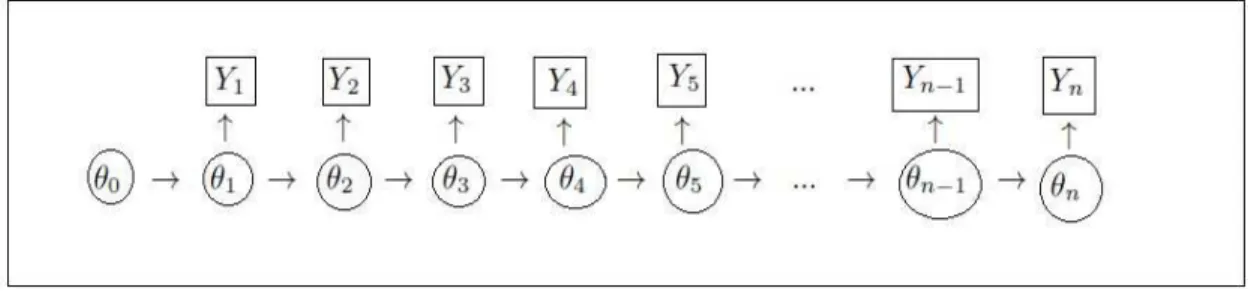
The dynamic linear models can be represented graphically as shown in Figure 3.1, that is, Yt, t = 1, ..., n, a random component is related to a parameter θt, and these parameters being stochastically related. Specifically, in the dynamic generalized linear model the random component is random variables which distribution is a member of the uniparametric exponential family, and it is related to the parameter θt through a link function.
Chapter 4
Product Partition Model
Once time series data is in study, it is reasonable to think about change point problem, result of some intervention that can change the structure of the series and provide a clustering structure. An attractive tool to work with this kind of problem was proposed by Hartigan (1990), known as the product partition model (PPM), which allowed the data to weight the partitions likely to hold, and assumed that observations in different components of random partitions of the data are independent given the partition. The work of Barry and Hartigan (1992) consider an approach were the PPM was defined in terms of a partition of a set of observations into contiguous blocks, wherein the partition has a prior product distribution, and given the partition, the parameters in different blocks have independent prior distributions, and is describe as follows.
Consider an observed time series Y = (Y1, ..., Yn), that is, a sequence of observations
at consecutive points in time, wherein, conditionally on θ1, ..., θn, has marginal densities
p1(Y1|θ1), ..., pn(Yn|θn).
LetT ={1, ..., n}be the index set of the observed time seriesY andρ={t0, t1, ..., tb}
a random partition of the setT∪{0}, with 0 =t0 < t1 < ... < tb =n. LetB be a random
variable which represents the number of blocks inρ.Then, the partitionρdivides the time series Y into B = b contiguous blocks denoted by Y(j)
ρ = (Ytj−1+1, ..., Ytj)
′, j = 1, ..., b. Letθk =θ(ρj)fortj−1+1≤k ≤tj be the parameters vector conditionally on the partition
ρ={t0, t1, ..., tb}.
Considerc(j)
ρ the prior cohesion associated with blockYρ(j), which represents the degree
of similarity among the observations Y(j)
ρ . In the time series context, as pointed out by
Loschi and Cruz (2002), the cohesion may be interpreted as the transition probabilities in the Markov chain defined by the endpoints of the blocks in ρ.
Following Loschi and Cruz (2002) we say that the random quantity (Y1, ..., Yn;ρ)
1. The prior distribution of ρ={t0, t1, ..., tb} is
p(ρ={t0, t1, ..., tb}) =
b
Q
j=1c
(j)
ρ
P
C
b
Q
j=1c
(j)
ρ
, (4.1)
where C is the set of all possible partitions of the set T into b contiguous blocks with endpoints t1, ..., tb satisfying the condition 0 = t0 < t1 < ... < tb = n, for all
b∈T;
2. Given the partitionρ={t0, t1, ..., tb}, the sequenceY1, ..., Ynhas joint density given
by
p(Y|ρ={t0, t1, ..., tb}) =
b
Y
j=1
p(Y(ρj)), (4.2) where
p(Y(ρj)) =
Z
p(Y(ρj)|θ(j)
ρ )p(θ
(j)
ρ )dθ
(j)
ρ , (4.3)
is the density of the random vector, with p(θ(j)
ρ ) being the block prior density for θ(j)
ρ .
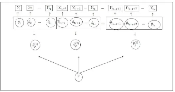
The graphical representation of the PPM is presented in Figure 4.1, that is, a random component (Y1, ..., Ytn) that givenθ1, ..., θtn are conditionally independent, and given the
partition the parametersθ(1)
ρ , ..., θρ(b)are independent. Loschi and Cruz (2002) emphasizes
that the formulation of the product partition model allows the parameters to be time varying, and then it is a kind of dynamic model.
The prior distribution for B, that is, the number of blocks in the partition is given by
p(B =b) ∝ X
C1
b
Y
j=1
c[ij−1ij], b∈T,
where C1 is the set of all partitions of T in b contiguous blocks with endpoint t1, ..., tb
satisfying the condition 0 =t0 < t1 < ... < tb =n.
Figure 4.1: Graphical representation of the product partition model.
It was also showed that the posterior distributions of θk, k = 1, ..., n is given by
p(θk|Y) = X
tj−1≤k≤tj
r∗(j)
ρ p(θ
(j)
ρ |Y
(j)
ρ ), (4.5)
and the posterior expectation, or product estimate, of θk is given by
E(θk|Y) = X
tj−1≤k≤tj
r∗(j)
ρ E(θ
(j)
ρ |Y
(j)
ρ ), (4.6)
where r∗(j)
ρ is the posterior relevance for the block j, which given by r∗(j)
ρ = P([tj−1tj]∈ρ|Y).
According to Hartigan (1990), for any probability model over partitions, the relevance probability is defined to be the probability that the blockY(ρj),j = 1, ..., b, is a component of the random partition ρ.
Although the product estimate in Equation (4.6) can be analytically calculated, it demands high computational efforts. Therefore, aiming to simplify the implementation of the method discussed previously, Barry and Hartigan (1993) suggested the use of an auxiliary random quantity Ui, in a Gibbs sampling scheme, given by
Ui =
1 if θi =θi+1,
which reflects whether or not a change point occurs at time i, for i = 1, ..., n−1. Once the vector U = (U1, ..., Un−1) is considered, the partition ρ is completely specified.
The Gibbs sampling is started with an initial value of U, that is, (U0
1, ..., Un0−1) and
then generating each vector (Us
1, ..., Uns−1), s≥1. Ther-th element of stepsis generated
from the following conditional distribution
Ur|Us
1, ..., Urs−1, Urs+1−1, ..., Uns−−11;Y,
r= 1, ..., n−1.
Consider the ratio presented bellow
Rr = P(Ur = 1|As;Y)
P(Ur = 0|Ar
s;Y)
,
r = 1, ..., n−1, where Ar
s = {U1s =u1, ..., Urs−1 =ur−1, Urs+1−1 =ur+1, ..., Uns−−11 =un−1}.
Therefore, is sufficient to generate the samples of U considering the ratio above and the following criterion of choosing the values Us
i, i= 1, ..., n−1
Us
r =
1 if Rr ≥ 1−u
u ,
0 otherwise,
where r= 1, ..., n−1 and u∼ U[0,1].
Following Barry and Hartigan (1993), a procedure to obtain the product estimates of
θk can be described as follows. For each partition (Us
1, ..., Uns−1), s ≥1, consider ˆθks the
estimates per block. The product estimates of θk, are approximated by
ˆ
θk =
M
P
s=1
ˆ
θks
M ,
Chapter 5
Dynamic Generalized Linear Model
via Product Partition Model
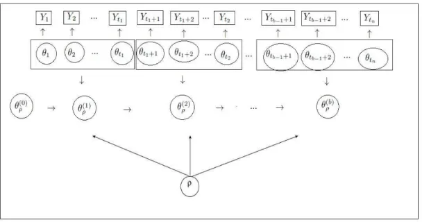
The dynamic generalized linear model, defined in Section 3.2, can be extended to allow for random partitions of the observed time series by using the product partition model, in or-der to accommodate time series in the uni-parametric exponential family of distributions with experiences changes point through time. The new class, which we shall refer here as dynamic generalized linear model via product partition model (DGLM via PPM), can be represented graphically as Figure 5.1. The PPM conditional independence of (Y1, ..., Ytn)
givenθ1, ..., θtn is conserved, but given the partitionρ the parametersθ
(1)
ρ , ...,θ
(b)
ρ will be
dependent. The formulation of the proposed model is given as follows.
Consider Y = (Y1, ..., Yn) an observed time series that has marginal distributions
p1(Y1|η1, V1), ..., pn(Yn|ηn, Vn), member of the uni-parametric exponential family, and
assume thatV1, ..., Vn is dropped from the list of conditioning arguments as it is assumed
to be known.
Let T = (1, ..., n) be the index set. Consider ρ = {t0, t1, ..., tb}, 0 = t0 < t1 <
... < tb = n a random partition of the set T ∪ {0}, which divides Y1, ..., Yn into B = b
contiguous blocks, with B being a random variable representing the number of blocks. Each block is denoted by Y(ρj) = (Ytj−1+1, ..., Ytj)
′ ≡ (Yj
1, ..., Yjnj)′, j = 1, ..., b, where nj
is the number of elements in the blockY(ρj). Notice thatYjk denotes thek-th element of the block Y(ρj).
Assume the following distribution of ρ ={t0, t1, ..., tb}
p(ρ={t0, t1, ..., tb}) =
b
Q
j=1c
(j)
ρ
P
C
b
Q
j=1c
(j)
ρ
, (5.1)
wherec(j)
ρ denotes the prior cohesion associated with the blockY
(j)
ρ and C is the set of all
possible partitions of the setT intobcontiguous blocks with endpointst1, ..., tb satisfying
the condition 0 =t0 < t1 < ... < tb =n, for all b∈T.
The prior distribution for B, that is, the number of blocks in the partition is given by
p(B =b) ∝ X
C1
b
Y
j=1
c[ij−1ij], b∈T,
where C1 is the set of all partitions of T in b contiguous blocks with endpoint t1, ..., tb
satisfying the condition 0 =t0 < t1 < ... < tb =n.
Suppose that a set of independent explanatory variables, denoted by Fjk, k = 1, ..., nj, j = 1, ..., b, where Fjk is p-dimensional vector, known as design vector, is
ob-served forYjk. Following West et al. (1985) it assumed thatYjk is related toFjk through
an observational model given by
g(ηjk) = λjk = F′jkθ(ρj), (5.2) whereg(ηjk) is a known, continuous and monotonic function mappingηjk to the real line.
Given ρ, θρ = (θ(1)ρ ,θ
(2)
ρ , ...,θ
(b)
ρ ), where θ
(j)
ρ is the state vector associated with the
conjugate prior distribution, denoted by ηjk ∼ CF(rjk, sjk), given by
p(ηjk) = c(rjk, sjk) exp{rjkηjk−sjka(ηjk)}, (5.3) where CF denotes the conjugate family and the hyperparametersrjk andsjk are defining quantities obtained from the moments ofg(ηjk) =F′jkθρ(j), andc(rjk, sjk) is a normalizing constant.
Therefore, conditionally onρ={t0, t1, ..., tb}the observations have the following joint
density
p(Y|ρ={t0, t1, ..., tb}) =
b
Y
j=1
p(Y(ρj)), (5.4) where
p(Y(ρj)) =
nj
Y
k=1
Z
p(Yjk|ηjk)p(ηjk)dηjk
=
nj
Y
k=1
c(rjk, sjk)b(Yjk, Vjk)
Z
exp{V−1
jk [Yjkηjk − a(ηjk)]}exp{rjkηjk−sjka(ηjk)} dηjk
=
nj
Y
k=1
c(rjk, sjk)b(Yjk, Vjk)
c(rjk +φjkYjk, sjk +φjk),
is the predictive distribution of the observations in the Y(j)
ρ block, known as data
fac-tor. For all distributions member of the exponential family c(.) and c(.) are determined functions, thus the predictive function can also be determined in all cases.
The posterior distribution of ρ={t0, t1, ..., tb} is given by
p(ρ={t0, t1, ..., tb}|Y) =
b
Q
j=1c
∗(j)
ρ
P
C
b
Q
j=1c
∗(j)
ρ ,
where c∗(j)
ρ =c(ρj)p(Y(
j)
ρ ) is the posterior cohesion.
The posterior distribution of B have the same form of the prior distribution, using the posterior cohesion for thej-th block.
product partition model.
Assume that the state parameters from different blocks are related through the evo-lution equation:
θρ(j) = Gjθρ(j−1)+wj, (5.5)
where Gj is a known evolution matrix of θ(ρj) and wj is an evolution error associated to
the block Y(ρj) having mean vector equal to zero and covariance matrix equal toWj.
The prior for the state vector, that is, θ(ρj), will be specified as usual in dynamic modeling. Let D(ρj) be the data information available up to the block j. The model specification is completed by the following posterior distribution
(θ(ρj−1)|D(ρj−1)) ∼ (mj−1,Cj−1).
Then, using the evolution equation in (5.5), the prior distribution for θ(ρj) obtained is (θ(ρj)|Dρ(j−1)) ∼ (aj,Rj),
where
aj =Gjmj−1 and Rj =GjCj−1G′j +Wj.
Denote by D(ρj−1;k−1) the set of all information available until the block j−1 and the proceed information up to the elementk−1. Assume the following joint prior distribution for λjk and θ(ρj)
λjk θ(ρj)
D(ρj−1;k−1)
∼ fjk ajk ,
qjk F′kRjk
RjkFk Rjk
(5.6)
where fjk =F′kajk and qjk =F′kRjkFk.
The one-step ahead forecast distribution is given by
p(Yjk|Dρ(j−1;k−1)) = c(rjk, sjk)b(Yjk, Vjk)
c(rjk+φjkYjk, sjk+φjk) (5.7)
The posterior distribution for ηjk is given by
p(ηjk|Dj−1;k) = c(rjk+φjkYjk, sjk+φjk) exp[(rjk+φjkYjk)ηjk − (sjk+φjk)a(ηjk)]. (5.8)
Hence, we are able to update the state parameter as it is usually done in DGLM frame-work. That is, (θ(ρj)|D(ρj−1;k−1)) ∼ (ajk,Rjk) is updated into (θ(ρj)|D(
j−1;k)
ρ ) ∼ (mjk,Cjk),
where
mjk = ajk+RjkFjk(fjk∗ −fjk)/qjk, (5.10)
and
Cjk = Rjk−RjkFjkFjk′ Rjk(1−qjk∗ /qjk)/qjk. (5.11)
At the start of each blockYj
ρ the updating is performed by takingaj1 =aj,Rj1 =Rj and
Djρ−1;0 =Dj−1. Within each block it is assumed that there is no parametric evolution, and we take aj;k+1 =mjk and Rj;k+1 =Cjk until the data information of all elements of
the block is processed. Then, mj;nj =mj, cj,nj =Cj and D
j;nj
ρ = D(
j)
ρ and perform the
parametric evolution. This cycle is repeated until D(ρb)=D is processed. Example 5.1 The Poisson model
Assume a time series Yjk, k = 1, ..., nj, j = 1, ..., b, such that Yjk|µjk ∼ Poisson(µjk). From Table 2.1 it is known the canonical parameter and the function b(.), that is,
ηjk = lnµjk and b(Yjk, V) = 1
Yjk!.
The conjugate prior for ηjk = lnµjk is described in Example 2.3 as follows.
p(ηjk|rjk, sjk) = c(rjk, sjk) exp{rjkηjk −sjkeηjk}, with normalizing constant
c(rjk, sjk) =
Z
exp{rjkηjk −sjkeηjk} dηjk
−1
= s
rt
t
Γ(rt),
where, from Table 3.1, it is know that,
sjk = exp(−fjk)
qjk and rjk =
1
qjk.
That way, the predictive distribution of the observations in the Y(j)
p(Y(ρj)) =
nj
Y
k=1
c(rjk, sjk)b(Yjk, Vjk)
c(rjk +φjkYjk, sjk+φjk)
= s
rjk
jk Γ(rjk +Yjk)
(sjk + 1)rjk+YjkΓ(rjk)Yjk!
=
rjk+Yjk−1
Yjk
sjk sjk+ 1
!rjk
1
sjk + 1
!Yjk
.
From Table 3.1 we also have the following approximate values of
fjk∗ = ln
rjk+Yjk sjk + 1
!
and qjk∗ =
1
rjk +Yjk Assuming a discrete uniform prior distribution for ρ, that is c(j)
ρ = 1 ∀j, the Gibbs sampling scheme described in Chapter 4 may be executed in order to obtain some inference about the partition. Then, given the partition, and computed the approximate values of rjk, sjk, f∗
jk and q∗jk, the DGLM inference about the state vector as Equations (5.10) and (5.11), and future observations as Equation (5.7) may be proceed.
In Tables 2.1 and 3.1 we presented the values of the functions c(.) and b(.), and the approximate values of rjk, sjk, f∗
jk and qjk∗ , for some distributions in the uni-parametric
exponential family. Then, for these distributions we are able to provide the DGLM via PPM inference as in Example 5.1.
5.1
Model comparison
In Bayesian context, the Bayes Factor (BF) and the Posterior Model Probability (PMP) (Kass and Raftery, 1995, see) are popular measures for model comparison and selection. We briefly describe how the BF and the PMP can be computed in the DGLM via PPM framework.
Comparing Mi, i = 1, ..., M and 2< M < ∞, models procedure consists, usually, of
computing the PMP for each model, and the criterion of selection is based on the model with highest PMP. The posterior probability of a modelMi given the dataY is given by
Bayes theorem
where p(Mi) is the prior probability associated to model Mi, satisfying PMi=1p(Mi) = 1
and p(Y|M) is the corresponding marginal distribution of Y.
LetMρandM0be the DGLM via PPM and the DGLM, respectively. When the model
selection consists in the choice between two models we may assess the Bayes factor, given by
BF(Mρ,M0) =
p(Y|Mρ) p(Y|M0)
=
P
ρ
R
p(ηρ|Y, ρ,Mρ)p(Y, ηρ, ρ,Mρ)p(ρ|Y)dηρ
R
p(η0|Y,M0)p(Y, η0,M0)dη0
.
Notice that the marginal distribution p(Y|Mρ) is obtained by firstly computing the
marginal distribution of Y conditioning on the partitions, and then averaging over all the partitions. The marginal distribution p(Y|M0) is obtained straightforwardly.
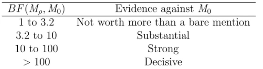
Kass and Raftery (1995) emphasizes that the Bayes Factor is a summary of the evidence provided by the data in favor of one model, as opposed to another, and presented a suggested scale to interpret it, showed in Table 5.1.
BF(Mρ,M0) Evidence againstM0
1 to 3.2 Not worth more than a bare mention 3.2 to 10 Substantial
10 to 100 Strong
>100 Decisive
Chapter 6
Application
In this chapter we present an analysis of two real time series data sets, already discussed in the literature, aiming to illustrate the usefulness of the proposed model, DGLM via PPM, and compare its inference to the DGLM inference. For both cases we provide a sensitivity analysis for different choices of the discount factor δ.
The Gibbs sampling scheme suggested by Barry and Hartigan (1993), and described in Chapter 4, was used to obtain some inference about the partition. Single chains of size 45,000 were considered. Posterior samples of size 4,000 were obtained after consid-ering a burn-in period of 5,000 iterations and a lag of 10 to eliminate correlations. We assumed that the prior cohesionc(j)
ρ = 1, j = 1, ..., b, implying in a discrete uniform prior
distribution for ρ={t0, t1, ..., tb}.
Prior elicitation for the state parameter θ is given by (θ(1)ρ |D(0)ρ ) ∼ [0,100Ip]. We
set the evolution matrix Gj = Ip, j = 1, ..., b, assuming then a random walk for the
parametric evolution. The specification of the evolution covariance matrices Wj was made according to the discount factor strategy. In this casep= 1, due to the absence of explanatory variables in both data sets. The computational procedures were implemented in R Core Team (2013).
6.1
APCI Data
households and utilities. When the APCI rises, means that these items will suffer a price adjustment up, that is inflation. When the APCI decreases, it does not mean that these items will have a price decrease, but that the prices rose less then the previous period. Only when the APCI is negative, we have a price decrease, that is deflation. The government utilizes it to check if the established inflation goal is being fulfilled.
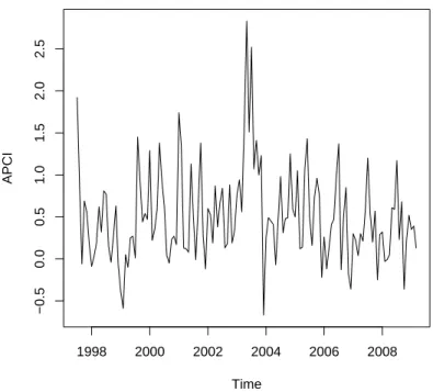
In this work we used the APCI series measured monthly in Belo Horizonte area, from the period of July, 1997 to June, 2008, resulting in 132 observations, which was previously analyzed in the work of Santos et al. (2010), presented in Figure 6.1. It can be observed an intervention around October, 2002, which occurred due to the concerns in the economy after the election of President Lula. We assumed that the series is Gaussian distributed.
Time
APCI
1998 2000 2002 2004 2006 2008
−0.5
0.0
0.5
1.0
1.5
2.0
2.5
Figure 6.1: APCI series.
highest posterior probability, except that in this case δ = 0.9 have a higher probability than the other values at left.
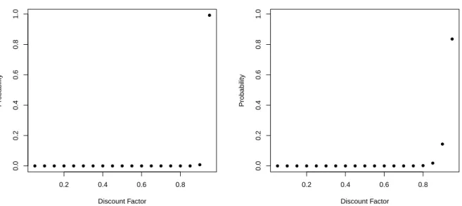
Table 6.1 provides the Bayes factor for the DGLM via PPM over the DGLM for the discount factors considered. We can observe the superiority of the DGLM via PPM over the DGLM, which is classified, for the discount factors values smaller or equals to 0.90 as decisive, and for the discount factor equals to 0.95 as substantial, following the interpretation scale presented in Table 5.1. This superiority is confirmed in Figure 6.3 when analyzing the posterior model probability for the DGLM and the DGLM via PPM. We observe that for δ ≤ 0.8, the PMP of both models are close to zero. For δ > 0.8 the models are more probables with the DGLM via PPM having bigger probabilities compared to the DGLM. The model with highest PMP is the DGLM via PPM with discount factor equal to 0.95.
● ● ● ● ● ● ● ● ● ● ● ● ● ● ● ● ● ● ●
0.2 0.4 0.6 0.8
0.0
0.2
0.4
0.6
0.8
1.0
Discount Factor
Probability
● ● ● ● ● ● ● ● ● ● ● ● ● ● ● ● ● ●
●
0.2 0.4 0.6 0.8
0.0
0.2
0.4
0.6
0.8
1.0
Discount Factor
Probability
δ Bayes Factor δ Bayes Factor δ Bayes Factor 0.05 3.48e+166 0.40 8.45e+36 0.75 5.86e+07 0.10 6.57e+122 0.45 3.74e+30 0.80 3.96e+05 0.15 6.71e+96 0.50 1.85e+25 0.85 5.45e+03 0.20 2.82e+78 0.55 4.25e+20 0.90 1.32e+02 0.25 3.76e+65 0.60 4.37e+16 0.95 6.11e+00 0.30 8.10e+53 0.65 1.86e+13
0.35 7.54e+44 0.70 2.17e+10
Table 6.1: Bayes Factor for different choices of δ with APCI data.
● ● ● ● ● ● ● ● ● ● ● ● ● ● ● ● ● ●
●
0.2 0.4 0.6 0.8
0.0
0.2
0.4
0.6
0.8
1.0
Discount Factor
Probability
Figure 6.3: Posterior model probabilities for DGLM via PPM (solid circle) and for DGLM (asterisk symbol) with the APCI data.
We concentrate our analysis, from now on, on making inferences for the DGLM and the DGLM via PPM based on the results for δ = 0.95, since it was the discount factor value with highest posterior model probability for both models.
have a common state parameter for observations in the same block. Hence, in this case, we expect a smoother behavior of the estimated posterior mean as, indeed, observed. Furthermore, in Figure 6.4 we observe that the estimated values of the DGLM via PPM follows well the estimated values of the DGLM.
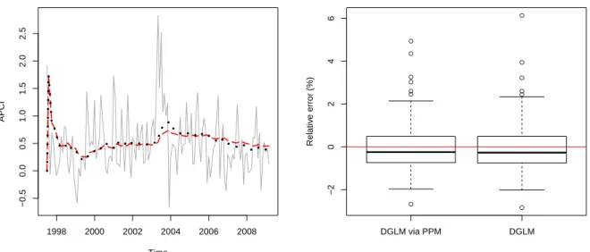
The forecast of the APCI series considering δ = 0.95, and its relative forecast error is showed in Figure 6.5. The forecasting was obtained by the mean of the estimated forecasts obtained for each partition generated. The over smoothed behavior of the forecast was expected due to the choice of discount close to one. This choice means that a high amount of information is being allowed to pass from time t−1 to time t, and implies that the evolution error is close to zero. This behavior of the parametric evolution implies that we have smoother forecasts. Nevertheless, this does not indicate a bad adjustment. Indeed, we have evidences of a good adjustment when looking the relative forecast errors.
Time
1998 2000 2002 2004 2006 2008
0.5
1.0
1.5
Figure 6.4: Posterior mean of the state parameter of the DGLM via PPM (solid line) and DGLM (dashed line), forδ = 0.95.
Time
APCI
1998 2000 2002 2004 2006 2008
−0.5 0.0 0.5 1.0 1.5 2.0 2.5 ● ● ● ● ● ● ● ● ● ● ● ● ●
DGLM via PPM DGLM
−2 0 2 4 6 Relativ
e error (%)
Figure 6.5: Forecast of the APCI series for the DGLM (pointed line) and DGLM via PPM (dashed line), and the relative forecast error for δ= 0.95 (right).
0 1000 3000
50 60 70 80 90 Iterations
Histogram of b
b
Frequency
50 60 70 80 90
0 200 400 600 800 1000 1200
One advantage of the proposed model is that we are able to make inferences about the partition as well the number of blocks. In Figure 6.7 we plotted the most probable number of blocks for both discount factors considered in order to investigate the behavior of the number of blocks in the partitions according to the choice discount factor. We observe that the number of blocks has a crescent behavior as the discount factor increase.
● ●
● ●
● ●
● ● ●
● ● ●
● ● ● ●
● ●
●
5 10 15 20 25 30
0.2
0.4
0.6
0.8
Number of blocks
Discount F
actor
Figure 6.7: Most probable number of blocks for the discount factors considered with the APCI series
Aiming to investigate more about the partitions provided, we displayed in Figure 6.8 the change point probability in the DGLM via PPM, with δ= 0.95. As it is well known, from the series, was expected that the model gives more probability to the observations around October, 2002 be a change point, due to the some economic changes related to the election of the President Lula. But, we observed that the model with this discount factor was given probability around 0.5 for all observations to be a change point. This behavior was not expected and it is not satisfactory from the inferential point of view.
Time
Probability
1998 2000 2002 2004 2006 2008
0.0
0.1
0.2
0.3
0.4
0.5
Figure 6.8: Change point probability for δ= 0.95.
year of 1999, when the Brazilian Central Bank changed the exchange rate regime. When