The CarboCount CH sites: characterization of a dense greenhouse gas observation network

(1)

ACPD

15, 12911–12956, 2015

Greenhouse gas observation network

characterization

B. Oney et al.

Title Page

Abstract Introduction

Conclusions References

Tables Figures

◭ ◮

Back Close

Full Screen / Esc

Printer-friendly Version Interactive Discussion

Discussion

P

a

per

|

Discussion

P

a

per

|

Discussion

P

a

per

|

Discussion

P

a

per

|

Atmos. Chem. Phys. Discuss., 15, 12911–12956, 2015 www.atmos-chem-phys-discuss.net/15/12911/2015/ doi:10.5194/acpd-15-12911-2015

This discussion paper is/has been under review for the journal Atmospheric Chemistry and Physics (ACP). Please refer to the corresponding final paper in ACP if available.

The CarboCount CH sites:

characterization of a dense greenhouse

gas observation network

B. Oney1,2, S. Henne1, N. Gruber2,3, M. Leuenberger4, I. Bamberger5,*, W. Eugster5, and D. Brunner1,2

1

Empa, Lab. for Air Pollution/Environmental Technology, Dübendorf, Switzerland 2

ETH Zurich, Center for Climate Systems Modeling, Zurich, Switzerland 3

ETH Zurich, Inst. of Biogeochemistry und Pollutant Dynamics, Zurich, Switzerland 4

Univ. of Bern, Physics Inst., Climate and Environmental Division, and Oeschger Centre for Climate Change Research, Bern, Switzerland

5

ETH Zurich, Inst. of Agricultural Sciences, Zurich, Switzerland *

now at: Karlsruhe Institute of Technology KIT Institute of Meteorology and Climate Research Atmospheric Environmental Research (IMK-IFU) Kreuzeckbahnstraße 19, 82467

Garmisch-Partenkirchen, Germany

Received: 24 January 2015 – Accepted: 25 March 2015 – Published: 4 May 2015

Correspondence to: D. Brunner ([email protected])

(2)

ACPD

15, 12911–12956, 2015

B. Oney et al.

Title Page

Tables Figures

◭ ◮

Back Close

Full Screen / Esc

Discussion

P

a

per

|

Discussion

P

a

per

|

Discussion

P

a

per

|

Discussion

P

a

per

|

Abstract

We describe a new rural network of four densely placed (<100 km apart), continuous atmospheric carbon (CO2, CH4, and CO) measurement sites in north-central

Switzer-land and analyze their suitability for regional-scale (∼100 to 500 km) carbon flux stud-ies. We characterize each site by analyzing surrounding land cover, observed local

5

meteorology, and sensitivity to surface fluxes, as simulated with the Lagrangian parti-cle dispersion model FLEXPART-COSMO.

The Beromünster measurements are made on a tall tower (212 m) located on a gen-tle hill. At Beromünster, regional CO2 signals (measurement minus background) vary

diurnally from−4 to+4 ppmv on average, and are simulated to come from nearly the

10

entire Swiss Plateau, where 50 % of surface influence is simulated to be within 130 to 260 km distance. The Früebüel site measurements are made 4 m above ground on the flank of a gently sloping mountain. Nearby (<50 km) pasture and forest fluxes exert the most simulated surface influence, except during convective summertime days when the site is mainly influenced by the eastern Swiss Plateau, which results in summertime

15

regional CO₂ signals varying diurnally from −5 to +12 ppmv and elevated summer daytime CH4 signals (+30 ppbv above other sites). The Gimmiz site measurements

are made on a small tower (32 m) in flat terrain. Here, strong summertime regional sig-nals (−5 to+60 ppmv CO₂) stem from large, nearby (<50 km) crop and anthropogenic fluxes of the Seeland region, except during warm or windy days when simulated

sur-20

face influence is of regional scale (<250 km). The Lägern-Hochwacht measurements are made on a small tower (32 m) on top of the steep Lägern crest, where simulated surface influence is typically of regional scale (130 to 300 km) causing summertime regional signals to vary from−5 to+8 ppmv CO2. Here, considerable anthropogenic

influence from the nearby industrialized region near Zurich cause the average

win-25

tertime regional CO₂ signals to be 5 ppmv above the regional signals simultaneously measured at Früebüel site.

(3)

ACPD

15, 12911–12956, 2015

B. Oney et al.

Title Page

Tables Figures

◭ ◮

Back Close

Full Screen / Esc

Discussion

P

a

per

|

Discussion

P

a

per

|

Discussion

P

a

per

|

Discussion

P

a

per

|

We find that the suitability of the datasets from our current observation network for regional carbon budgeting studies largely depends on the ability of the high-resolution (2 km) atmospheric transport model to correctly capture the temporal dynamics of the stratification of the lower atmosphere at the different sites. The current version of the atmospheric transport model captures these dynamics well, but it clearly reaches its

5

limits at the sites in steep topography, and at the sites that generally remain in the surface layer. Trace gas transport and inverse modeling studies will be necessary to determine the impact of these limitations on our ability to derive reliable regional-scale carbon flux estimates in the complex Swiss landscape.

1 Introduction

10

The exchange of carbon dioxide (CO2) with the terrestrial biosphere dominates the

ob-served year-to-year variability in the global carbon sinks (Battle et al., 2000; Sarmiento et al., 2010; Le Quéré et al., 2010) even though land surfaces cover only 30 % of the Earth’s surface area. Yet, our ability to quantify this variability in the net terrestrial car-bon flux directly from observations has remained limited (Ciais et al., 2014). As a result,

15

in most attempts to determine the global carbon budget, the net terrestrial carbon flux is estimated as the difference between the observed atmospheric carbon growth rate, and the sum of oceanic and anthropogenic carbon fluxes (Sarmiento et al., 2010; Le Quéré et al., 2013). Additionally, the lack of understanding of the feedbacks between climate change and the terrestrial biosphere translates into one of the greatest

un-20

certainties of future climate change projections (Heimann and Reichstein, 2008). An important step toward the reduction of this uncertainty is a better understanding of how the terrestrial biosphere responds to climatic fluctuations and trends. As the processes governing this response are inherently local to regional, this requires the determination of terrestrial carbon fluxes at high spatial resolution (Gerbig et al., 2009).

25

(4)

ACPD

15, 12911–12956, 2015

B. Oney et al.

Title Page

Tables Figures

◭ ◮

Back Close

Full Screen / Esc

Discussion

P

a

per

|

Discussion

P

a

per

|

Discussion

P

a

per

|

Discussion

P

a

per

|

that permit the determination of fluxes at continental scales (Gerbig et al., 2003a), and eddy covariance-based surface flux measurements that have a small-scale (∼1 km) footprint (Baldocchi et al., 2001). This leaves an obvious gap at intermediate scales (10 to 10 000 km), which clearly needs to be filled in order to reliably determine the terrestrial carbon budget (Ciais et al., 2014). The establishment of the North American

5

(Bakwin et al., 1998) and European (http://www.chiotto.org/; Vermeulen et al., 2004) tall tower networks represented a big step in this direction, but the high spatial het-erogeneity of land cover and the correspondingly large variations in the CO2 fluxes

require even denser observation networks, especially in order to target regional scale (<1000 km) carbon fluxes (Dolman et al., 2009; Lauvaux et al., 2012). The spatial

10

density of a measurement network required to resolve the spatial distribution of carbon fluxes is dependent on the region of interest and the corresponding carbon flux signa-tures, and largely remains an open question (Groenendijk et al., 2011; Lauvaux et al., 2012).

Short-term measurement campaigns, such as the Large-Scale

Biosphere-15

Atmosphere Experiment in Amazonia (Andreae et al., 2002), the CO2 Budget and

Rectification Airborne study (Gerbig et al., 2003b), and the CarboEurope Regional Ex-periment Strategy study (Dolman et al., 2006), have demonstrated the value of regional scale (<1000 km) datasets, but lacked the temporal coverage for the calculation of an-nual carbon budgets and the investigation of seasonal carbon flux variation. The

Mid-20

Continent Intensive (MCI) measurement campaign attempted to oversample the US upper midwest over a longer period of time (2007–2009; Miles et al., 2012), but even with an average distance of approximately 188 km between eight towers, Lauvaux et al. (2012) found that the spatial density of the measurement network was insufficient to consistently retrieve the spatial distribution of carbon fluxes.

25

The CarboCount CH project (http://www.carbocount.ch) was designed to overcome some of these limitations. It aims to quantify terrestrial carbon fluxes at high tem-poral and spatial resolution for multiple years through a combination of greenhouse gas concentration measurements and high-resolution atmospheric transport

(5)

ACPD

15, 12911–12956, 2015

B. Oney et al.

Title Page

Tables Figures

◭ ◮

Back Close

Full Screen / Esc

Discussion

P

a

per

|

Discussion

P

a

per

|

Discussion

P

a

per

|

Discussion

P

a

per

|

ing. Four greenhouse gas measurement sites have been established in the Swiss Plateau (Fig. 1), which is a densely settled, partly flat and hilly region between the Alps and Jura mountains approximately 50 km by 200 km in size with an average altitude of ∼450 m a.s.l. The measurement sites are located in rural areas and the average distance between sites is 85 km. The main goal of the CarboCount CH project is to

5

better understand surface fluxes of carbon, which for carbon dioxide (CO2) mainly

con-sist of anthropogenic emissions and biospheric activity, and for methane (CH₄) mainly (∼80 %) consist of agricultural emissions (Hiller et al., 2014).

The CarboCount CH measurement network includes measurement sites in com-plex terrain, which warrants the use of high resolution transport models (Pillai et al.,

10

2011). A measurement site’s local environment, especially the topography and land cover within<3 km distance, exerts influence on the local meteorology and thereby largely determines the local surface influence on observed trace gas concentrations (Vesala et al., 2008). Currently, most surface flux estimation studies usually use only afternoon measurements when the ABL is thickest and well-mixed to reduce the

sensi-15

tivity to errors in the representation of the ABL by the underlying atmospheric transport models (Gerbig et al., 2009; Pillai et al., 2012; Kretschmer et al., 2014). Owing to the requirement of high resolution transport models to represent the winds in complex ter-rain, many inverse modeling studies do not use trace gas concentration measurements from mountain sites.

20

The purpose of this study is to characterize the CarboCount CH observation net-work. We describe the local environment of each of the four measurement sites and investigate how much the local environment influences meteorology and greenhouse gas measurements. Furthermore, we assess the sensitivity of each measurement site to regional surface fluxes with the Lagrangian particle dispersion model

FLEXPART-25

(6)

informa-ACPD

15, 12911–12956, 2015

B. Oney et al.

Title Page

Tables Figures

◭ ◮

Back Close

Full Screen / Esc

Discussion

P

a

per

|

Discussion

P

a

per

|

Discussion

P

a

per

|

Discussion

P

a

per

|

tion content of each site’s measurements and establish potential guidelines for future transport and inverse modeling studies.

2 Data and methods

2.1 Measurement data

The four measurement sites of the CarboCount CH network (Fig. 1 and Table 1) were

5

equipped with PICARRO (Santa Clara, California, USA) cavity ring-down spectrom-eters for greenhouse gases measurements (Crosson, 2008; Rella et al., 2013). Ad-ditionally, meteorological variables including horizontal wind, humidity, dewpoint, and temperature were measured at all four sites. At Beromünster (BEO), air was sampled from five different heights (212, 132, 72, 45, and 12 m a.g.l.), and carbon dioxide (CO2),

10

methane (CH4), water (H2O) and carbon monoxide (CO) were measured with a

PI-CARRO G2401 analyzer. Meteorology was measured at all heights with Gill MetPak II Remote weather stations (Gill Instruments Ltd., Hampshire, UK). Data used in this study were taken from the highest height. At Gimmiz (GIM), CO2, CH4, and H2O

con-centrations were measured with a PICARRO G2301, and CO with a Horiba APMA360,

15

which were taken at 32 m a.g.l. The same meteorology instrumentation at Beromünster was employed here. At Früebüel (FRU), which is also a Swiss Fluxnet site (Zeeman et al., 2010), CO₂, CH₄, and H₂O concentrations were measured with a PICARRO G2301 at 4 m a.g.l. and meteorology variables were measured at a height of 2 m a.g.l. (Bamberger et al., 2015). On the 32 m tower at Lägern-Hochwacht (LAE), CO2, CH4,

20

CO, and H₂O concentrations were measured with a PICARRO G2401. Here, Me-teoSwiss measured the following meteorological variables: wind (Vaisala WA25 Wind Set, Vaisala Inc., Helsinki, Finland), temperature and humidity (Vaisala HMP155), pres-sure (Vaisala PTB-220).

CO₂and CH₄measurements were calibrated against the corresponding international

25

reference scales: WMO X2007 for CO2 (Zhao and Tans, 2006), and WMO X2004 for

(7)

ACPD

15, 12911–12956, 2015

B. Oney et al.

Title Page

Tables Figures

◭ ◮

Back Close

Full Screen / Esc

Discussion

P

a

per

|

Discussion

P

a

per

|

Discussion

P

a

per

|

Discussion

P

a

per

|

CH₄(Dlugokencky et al., 2005). The calibration of target gas measurements – not used for the determination of calibration coefficients – suggests an accuracy of the CO2

and CH4measurements of∼0.07 ppmv and∼0.5 ppbv, respectively, computed as the

10 day averaging window RMSE of individual target measurements during the study period. Except for Früebüel, CO was also continuously measured, and was determined

5

to have an accuracy of ∼4 ppbv, computed as the 10 day averaging window target RMSE. Measurements were summarized to hourly averages for the one-year period from 1 March 2013 to 28 February 2014 considered in this study.

In order to derive regional signals – the anthropogenic and biospheric contributions within the simulation domain – of the trace gas concentrations at each site, a

back-10

ground concentration was estimated and subtracted from the measurements. The background concentration was estimated using the “robust extraction of baseline sig-nal” method (Ruckstuhl et al., 2012) from measurements at the high Alpine research station Jungfraujoch, which mainly samples free tropospheric air (Zellweger et al., 2003; Henne et al., 2010). Measurements at Jungfraujoch were made with a PICARRO

15

G2401 analyzer and referenced to the same calibration scales (Schibig et al., 2015). We investigated the validity of the assumption that this background concentration esti-mate corresponds to background concentrations by comparing with the NOAA’s Marine Boundary Layer reference (MBL1) at the corresponding latitude. We found them to be very similar (not shown), but the annual peak-to-peak amplitude of the Jungfraujoch

20

background concentration estimate (∼8 ppmv) is less than that of the MBL estimate (∼14 ppmv). However, the qualitative purpose of considering regional signals in this study remains una_ffected by these di_fferences.

For Switzerland, agricultural CH4 emissions constitute more than 80 % of the total

emissions and show high spatial variation, but their temporal variations are small and

25

predominantly seasonal (Hiller et al., 2014), due to seasonal relocation of cattle. There-fore, within a season, variations of methane concentrations serve as an atmospheric tracer and specifically as a proxy for the effect of the diurnally varying ABL.

1

(8)

ACPD

15, 12911–12956, 2015

B. Oney et al.

Title Page

Tables Figures

◭ ◮

Back Close

Full Screen / Esc

Discussion

P

a

per

|

Discussion

P

a

per

|

Discussion

P

a

per

|

Discussion

P

a

per

|

2.2 COSMO meteorology and FLEXPART-COSMO simulations

The sensitivity of the four measurement sites to upwind surface fluxes was assessed using a Lagrangian particle dispersion model (LPDM) driven by meteorological fields from a high resolution numerical weather prediction (NWP) model. As input for the transport simulations we used hourly analysis fields from the operational weather

fore-5

cast system of the Swiss national weather service MeteoSwiss, which is based on the NWP model COSMO. COSMO is a state-of-the-art non-hydrostatic, limited-area NWP model (Baldauf et al., 2011) developed by the Consortium for Small-Scale Modeling under the guidance of the German weather service DWD (Offenbach, Germany). It is the operational weather forecast model of the national weather services in Germany,

10

Greece, Italy, Poland, Romania, and Russia. In the version COSMO-CLM (Climate Lim-ited area Modeling), optimized for climate simulations, it is used by a wide community of regional climate modelers (http://www.clm-community.eu).

The operational setup for COSMO simulations of MeteoSwiss includes two nested domains. The outer domain covers large parts of Europe at about 7 km×7 km resolution

15

(COSMO-7). The inner domain covers the Alpine region including Switzerland, Austria and parts of Germany, France and Italy at about 2 km×2 km resolution (COSMO-2). COSMO-7 is driven by European Center for Medium Range Weather Forecast (ECMWF) analysis fields of ECMWF’s global IFS model and provides the boundary conditions for the COSMO-2 simulation. Hourly analysis fields are produced for both

20

model domains applying the observational nudging technique (Schraff, 1997) to sur-face observations of pressure, relative humidity and wind. Similarly, measurements of the same variables plus ambient temperature as taken with sondes and profilers are also assimilated. In addition, a latent heat nudging scheme (Stephan et al., 2008) is used for the COSMO-2 domain to incorporate radar derived rain rates2.

25

COSMO-2 provides the high resolution necessary to represent the complex topog-raphy in the alpine area and the topogtopog-raphy-induced mesoscale weather patterns. In

2

For more details see: http://cosmo-model.org/content/tasks/operational/default.htm.

(9)

ACPD

15, 12911–12956, 2015

B. Oney et al.

Title Page

Tables Figures

◭ ◮

Back Close

Full Screen / Esc

Discussion

P

a

per

|

Discussion

P

a

per

|

Discussion

P

a

per

|

Discussion

P

a

per

|

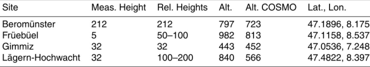
order to evaluate the ability of COSMO-2 to represent the local meteorology at the four measurement sites, we interpolated COSMO-2 analysis fields horizontally to each site and vertically to 18 altitude levels between 10 and 3240 m abovemodelground. This al-lows us to compare COSMO-2 with meteorological measurements at different heights above ground. Furthermore, it allows assessing the effect of a mismatch between the

5

true altitude of a site and its representation in the model where the topography is smoothed due to the limited model resolution. Although the gentle hill at Beromün-ster and the flat area around Gimmiz are well represented, the model’s elevation at the mountain sites Früebüel and Lägern-Hochwacht are 169 and 274 m, respectively lower than the true elevation. Therefore, we compared COSMO-2 output at two different

10

levels, i.e., at the altitude of the measurement a.s.l. (“true”), and at the measurement height a. m. g. (“model”). The true altitudes and the corresponding model altitudes are summarized in Table 2.

Hourly COSMO analysis fields were used to drive o_ffline atmospheric transport sim-ulations with a modified version of the LPDM FLEXPART (Stohl et al., 2005).

FLEX-15

PART simulates the transport and dispersion of infinitesimally small air parcels (re-ferred to as particles) by advective as well as turbulent and convective transport. It can be run either in forward mode (source oriented, i.e. released from sources) or backward mode (receptor oriented, i.e. released backward from receptors). The ad-vective component is calculated from the 3-D wind fields provided by COSMO, and

20

the turbulent transport is based on the scheme of Hanna (1982), which diagnoses ABL and turbulence profiles for stable, neutral and unstable boundary layers based on Monin–Obukhov similarity theory. FLEXPART was modified to run directly on the na-tive grid of COSMO, which is a rotated longitude-latitude grid on a hybrid geometric (i.e. fixed in space) vertical coordinate system. The fact that the original FLEXPART

25

(10)

ACPD

15, 12911–12956, 2015

B. Oney et al.

Title Page

Tables Figures

◭ ◮

Back Close

Full Screen / Esc

Discussion

P

a

per

|

Discussion

P

a

per

|

Discussion

P

a

per

|

Discussion

P

a

per

|

Emanuel convection scheme (Forster et al., 2007). Convection is treated as a grid-scale process in COSMO-2 and, hence, no sub-grid convection parameterization is run in either COSMO or FLEXPART-COSMO for the 2 km×2 km domain. From all four sites, backward transport simulations with FLEXPART-COSMO were started every 3 h to trace the origin of the observed air parcels. In each simulation, 50 000 particles were

5

released from the site’s position at site-dependent heights above ground and traced backward in time over 4 days or until they left the simulation domain. The simulations were performed in a nested configuration with COSMO-2 providing the meteorological inputs for the inner domain and COSMO-7 for the outer domain once the particles left the COSMO-2 region. Simulated residence timesτ (s m3kg−1; described in Sect. 2.4)

10

were generated for two separate output domains: a high-resolution grid over Switzer-land at 0.02◦×0.015◦horizontal resolution extending from 4.97 to 11.05◦E and 45.4875 to 48.5475◦N, and a coarser European grid at 0.16◦×0.12◦resolution extending from −11.92 to 21.04◦E and 36.06 to 57.42◦N. Due to the relatively well represented to-pography at Beromünster and Gimmiz, we chose to release particles at the

measure-15

ment height above model ground level. The relatively poor representation of topog-raphy around Früebüel and Lägern-Hochwacht, however, led us to release particles from a layer between “true” and “model” height rather than from a single height. The particle release heights were chosen based on meteorological evaluation of COSMO presented below and are listed in Table 2.

20

2.3 Land cover dataset

In order to evaluate the sensitivity of the measurement sites to different land cover types (LCT), a dataset of fractional land cover was produced for the FLEXPART-COSMO output domains. The land cover data set consists of LCTs classified according to the land-unit/plant functional type approach used in the land surface model CLM4 (Bonan

25

et al., 2002; Lawrence et al., 2011). Two main sources of land cover data sets were used: the CORINE2006 European land cover data with a resolution of 100 m×100 m (EEA, 2007) and the MODIS MCD12Q1 IGBP land cover categorization (Friedl et al.,

(11)

ACPD

15, 12911–12956, 2015

B. Oney et al.

Title Page

Tables Figures

◭ ◮

Back Close

Full Screen / Esc

Discussion

P

a

per

|

Discussion

P

a

per

|

Discussion

P

a

per

|

Discussion

P

a

per

|

2010) for the reference year 2011 with a resolution of 500 m×500 m, at locations where CORINE2006 was unavailable. For simplification, we summed plant functional type fractions according to primary plant functional type e.g. temperate evergreen needle-leaf forest plus boreal evergreen needleneedle-leaf forest or temperate deciduous broadneedle-leaf shrub plus boreal deciduous broadleaf shrub. As expected, the temperate and boreal

5

climate zones comprise all of the simulation domain. Further simplifications of plant functional types were according to leaf phenology of forests; e.g. we summed decid-uous broad-leaf and deciddecid-uous needle-leaf forest land cover fractions. Furthermore, lakes and wetlands were summed to “Freshwater areas”, and the plant cover type “Bare” and glacier coverage were also summed to “Bare areas”.

10

2.4 Regional surface influence metrics

We define surface sensitivityτ₁₀₀ (s m3kg−1) as the residence time of the particles in a 100 m thick layer above model ground divided by the density of dry air in that layer. A layer thickness of 100 m was selected as a compromise between the requirement of selecting a height low enough to be always located in the well-mixed part of the ABL

15

and high enough to allow for a statistically sufficient number of particles in the layer. The results were largely insensitive to this choice as confirmed by comparing with results forτ₅₀ (50 m) andτ₂₀₀ (200 m). Maps of the total residence time summed over the (four-day) simulation period are commonly referred to as footprints and describe the sensitivity of a measurement site to upwind surface fluxes (Seibert and Frank,

20

2004). For this study only monthly or seasonally averaged residence times were used to characterize the surface influence of the four sites, and are hereafter referred to as mean surface sensitivities,τ. Further temporally averaged quantities also have an overline.

The spatial sum of monthly mean surface sensitivities, the total surface sensitivityTt,

25

(12)

ACPD

15, 12911–12956, 2015

B. Oney et al.

Title Page

Tables Figures

◭ ◮

Back Close

Full Screen / Esc

Discussion

P

a

per

|

Discussion

P

a

per

|

Discussion

P

a

per

|

Discussion

P

a

per

|

defined as

Tt=

X

i,j

τ_i_,_j, (1)

wherei andj are spatial indices.

Short-term variations in observed trace gas concentrations are mainly determined by upwind surface fluxes, which vary with the associated land cover type. In order to

5

investigate influence of di_fferent LCTs on each measurement site, monthly LCT con-tributions C_LCT were calculated as the weighted mean of LCT fractions f_LCT,_i_,_j over the FLEXPART output grid, using monthly mean surface sensitivities τ_i_,_j as weights (Eq. 2). With equal surface flux strengths, each LCT would constitute the respective fractionC_LCTof the observed signal.

10

C_LCT₌ 1 Tt

X

i,j

τ_i_,_j_·f_LCT,_i_,_j (2)

In order to better gauge the decrease of surface sensitivity with increasing distance, we define the radial surface sensitivityTk for a site as

Tk= 1 ∆d

X

i,j

τ_i_,_j ∀i,j: d_k< d_i_,_j < d_k_{+ ∆}d, (3)

where d_i_,_j is the great-circle distance of the grid cell with indices i and j from the

15

measurement’s site position, and the indexk defining a discrete distance bin of width

∆d.

In order to compare the area of surface influence of each site, we investigated cu-mulative surface sensitivities defined as

s(τ)=X

i,j

τ_i_,_j ∀i,j: τ_i_,_j > τ. (4)

20

(13)

ACPD

15, 12911–12956, 2015

B. Oney et al.

Title Page

Tables Figures

◭ ◮

Back Close

Full Screen / Esc

Discussion

P

a

per

|

Discussion

P

a

per

|

Discussion

P

a

per

|

Discussion

P

a

per

|

The area of surface influence is then defined as the region surrounding the site bounded by the isolineτ_s50, at which the cumulated surface sensitivity includes 50 % of the total surface sensitivity:

τ_s50:s(τ_s50)=0.5Tt. (5)

Similar metrics were computed by Gloor et al. (2001) using trajectory simulations.

5

They derived a concentration footprint from the decay of the correlation between popu-lation density, integrated along the trajectories, and C2Cl4measurements with

increas-ing distance from the measurement site. Although they showed the robustness of their methods, we argue that the independence of Tk and τ_s50 from trace gas measure-ments and associated surface fluxes constitutes an improvement of the definition of

10

the concentration footprint. Furthermore, the application of an LPDM model that better describes atmospheric transport and dispersion constitutes a clear improvement over their approach but comes at much higher computational cost.

3 Results and discussion

3.1 Local site characteristics

15

The Beromünster site is a 212 m tall, decommissioned radio tower located on a gentle hill in an agricultural area in central Switzerland with an elevation of 797 m a.s.l. at the base (Fig. 2). Several small farms are located in the vicinity of the tower, and the town of Beromünster (<7000 inhabitants) is approximately 2 km to the north. The adjacent valley bottoms are at an elevation of approximately 500 and 650 m a.s.l. Beromünster’s

20

surroundings consist of a mosaic of agricultural uses: crops, managed grasslands, and a forested area towards the south.

(14)

ACPD

15, 12911–12956, 2015

B. Oney et al.

Title Page

Tables Figures

◭ ◮

Back Close

Full Screen / Esc

Discussion

P

a

per

|

Discussion

P

a

per

|

Discussion

P

a

per

|

Discussion

P

a

per

|

agricultural land in the nineteenth century (Fig. 2). The town of Aarberg (<5000 inhab-itants) is at a distance of approximately 2 km to the southwest, and a farm is situated 200 m to the northeast. The flat area around Gimmiz mainly consists of agricultural plots of seasonal crops, known as the “vegetable garden” of Switzerland. Furthermore, the area directly surrounding Gimmiz is under groundwater protection and further

sur-5

roundings are under water protection, which means that cattle grazing and use of fer-tilizer is tightly regulated or forbidden.

About 30 km to the southwest of Beromüenster, Früebüel, a Swiss Fluxnet site (Zee-man et al., 2010), is located at an altitude of 987 m a.s.l. on the flank of the gently sloping pre-Alpine Zugerberg, some 500 m above the valley floor (Fig. 3). The region

10

consists of glacial lakes, managed forests and seasonal pastures. The city of Zug 10 km to the north and the small town of Walchwil 2 km to the southwest are the major nearby anthropogenic sources. A small farm is located approximately 300 m to the south. Sea-sonal pasture surrounds the site, and approximately 50 m to the west there is a small patch of forest, the canopy of which is higher than the measurement inlet at 4 m a.g.l.

15

The site Lägern-Hochwacht, a 32 m tall tower, is located on the east-west oriented mountain ridge Lägern at an altitude of 840 m a.s.l., and is north of the city of Zurich in the most industrialized and densely settled area of Switzerland (Fig. 3). The terrain falls offsteeply to the north and south from the site, and the Lägern crest extends about 10 km westwards at similar altitude. Lägern-Hochwacht is surrounded by deciduous

20

and coniferous forest with a maximal canopy height of 20 m.

Model topography and land cover

Although the main topographic features of Switzerland are represented, the spatial resolution of 2 km creates large di_fferences between true and model topography at the two mountain sites Früebüel and Lägern-Hochwacht (see Table 1 and Fig. 3, second

25

column). In the model topography, the general shape of the Zugerberg remains, but the site’s altitude is much lower (169 m). The steep Lägern crest is not identifiable in the model topography, and therefore the site’s model altitude is much lower (274 m). On the

(15)

ACPD

15, 12911–12956, 2015

B. Oney et al.

Title Page

Tables Figures

◭ ◮

Back Close

Full Screen / Esc

Discussion

P

a

per

|

Discussion

P

a

per

|

Discussion

P

a

per

|

Discussion

P

a

per

|

other hand, Beromünster’s altitude is slightly lower in the model topography (74 m), but the local topographical features remain identifiable. Furthermore, the plain topography surrounding Gimmiz compares well with the model topography, and the site’s model altitude is slightly higher (9 m).

The land cover in Switzerland is highly fragmented at scales smaller than 2 km

5

(Figs. 2 and 3, third column). The actual variety of land cover, specifically plant func-tional types, is usually highly simplified in land surface models. Groenendijk et al. (2011) concluded that this simplification may have significant consequences for re-gional carbon flux modeling, especially in highly heterogeneous landscapes, such as Switzerland. Therefore, the influence of local fluxes on measured concentrations will

10

still likely be di_fficult to simulate even at this relatively high resolution.

3.2 Local meteorology and diurnal cycle

The measured wind roses indicate frequent air flow channeling between the Jura moun-tain range and the Alps, resulting in either southwesterly or northeasterly wind direc-tions (Fig. 4). Früebüel is an exception, where the local environment likely redirects

15

prevailing winds. Due to the highest measurement altitude, Beromünster observed the highest windspeeds. At Gimmiz, lower windspeeds due to lower measurement alti-tude and high frequency of northeasterly winds, colloquially known as “Bise”, are mea-sured. Früebüel occasionally observes strong winds from southeasterly directions dur-ing Foehn events (Bamberger et al., 2015). Similar to Beromünster, Lägern-Hochwacht

20

observed high windspeeds, which were highly channeled from either northeast or southwest.

At Beromünster, the diurnal cycles of measured windspeed show higher values dur-ing nighttime than daytime indicatdur-ing presence in the mixed layer durdur-ing daytime and transition to the nocturnal residual layer during nighttime (Figs. 5 and 6). In summer,

25

(16)

cor-ACPD

15, 12911–12956, 2015

B. Oney et al.

Title Page

Tables Figures

◭ ◮

Back Close

Full Screen / Esc

Discussion

P

a

per

|

Discussion

P

a

per

|

Discussion

P

a

per

|

Discussion

P

a

per

|

responds temporally to that of summertime regional methane signals (∆CH₄), further indicating mixed layer influence. Summertime regional CO2signals (∆CO2) show only

a small diurnal (±4 ppmv) variability, which corresponds to the expectation of a weak signal from diurnal surface flux variations at the top of a tall tower (Andrews et al., 2014). Wintertime diurnal variability is hardly discernible in both CO2and CH4

concen-5

trations, indicating a weak influence of ABL dynamics.

At Gimmiz, the increase in windspeed during the day and decrease during the night indicates constant presence of the measurement inlet in the surface layer, contrary to Beromünster (Figs. 5 and 6). In summer and winter, CO2 and CH4 are negatively

correlated with windspeed, further emphasizing the influence of diurnal ABL dynamics.

10

The nighttime increase of more than 60 ppmv suggests rapid accumulation of respired

∆CO2 in the shallow nocturnal boundary layer. Nocturnal regional advection of∆CO2

may also contribute to the nighttime enrichment (Eugster and Siegrist, 2000), although low windspeeds at night suggest that the surface influence is limited to a few tens of kilometers from the site. Both the high wintertime CO2concentrations (30 ppmv above

15

background), and the high correlation between wintertime∆CH4 and ∆CO2 indicate

that wintertime diurnal ABL dynamics are responsible for observed diurnal variability. Please note that the winter was atypically mild (2.3◦C above the norm from 1961– 1990; MeteoSwiss, 2014) for regions north of the Alpine divide, which would have caused increased wintertime respiration, and contributed to the high observed CO₂

20

concentrations.

At Früebüel, the large magnitude in the temperature daily cycle, the low measured windspeeds, and the high humidity indicate strong surface influence (Figs. 7 and 8), and is consistent with the near-surface measurement height. During summer, CO2

concentrations decreased in the morning along with an increase in temperature and

25

humidity, both before windspeed increased. This typifies influence of photosynthetic activity, and further indicates strong local surface influence.

The second mountaintop site Lägern-Hochwacht shows a similar behavior to Beromünster with a delayed increase in daytime temperatures and higher windspeeds

(17)

ACPD

15, 12911–12956, 2015

B. Oney et al.

Title Page

Tables Figures

◭ ◮

Back Close

Full Screen / Esc

Discussion

P

a

per

|

Discussion

P

a

per

|

Discussion

P

a

per

|

Discussion

P

a

per

|

at night than during the day (Figs. 7 and 8). Especially during summer, the diurnal cy-cles of measured windspeed show higher values during nighttime than daytime, which indicates a shift from the mixed layer during daytime to the residual layer during night-time, and an increased influence of nocturnal jets. Specific humidity exhibits an in-crease between 06:00 and 09:00 UTC (07:00–10:00 LT) and a simultaneous dein-crease

5

in windspeed, further indicating a shift to the mixed layer. The delay in the decrease of

∆CO₂and peak of∆CH₄at 09:00 UTC indicate upward mixing of air containing noctur-nally accumulated CO2and CH4, which we also observe at Beromünster. On average,

the mixed layer begins to influence Lägern-Hochwacht measurements an hour earlier than at Beromünster. During winter, the additional 5 ppmv offset compared to Früebüel

10

in the flat diurnal cycle of _∆CO₂ and _∆CH₄ concentrations indicates nearby anthro-pogenic sources, and weak influence from ABL dynamics, respectively.

COSMO-2 meteorology evaluation

Beromünster’s simulated wind roses compare well with the observed wind roses, but high windspeeds are simulated too frequently (Fig. 4). Simulated and measured diurnal

15

cycles agree well in all seasons, and simulations at the measurement height above model ground level at 212 m agree slightly better (Figs. 5 and 6). Small differences from the measurements include an overestimation of windspeeds in the afternoon in summer, and a delayed and too small increase in temperature during winter.

At Früebüel, neither the dominating wind directions nor the wind speeds are well

re-20

produced by the COSMO-2 model suggesting strong localized influences on wind pat-terns. The lowest model output level (10 m a.g.l.) compares best with the near-surface meteorological characteristics of Früebüel. Because the model is evaluated at the cen-ter of the lowest model layer at about 10 m a.g.l. and the meteological measurements are closer to the surface at 2 m a.g.l., a general overestimation of windspeeds is

ex-25

(18)

ACPD

15, 12911–12956, 2015

B. Oney et al.

Title Page

Tables Figures

◭ ◮

Back Close

Full Screen / Esc

Discussion

P

a

per

|

Discussion

P

a

per

|

Discussion

P

a

per

|

Discussion

P

a

per

|

most notably in winter. On the other hand, simulated wintertime temperatures show a warm bias even at the true station height, well above the surface.

At Gimmiz, the simulated wind roses compare well, but a small bias in the north-eastern wind direction exists. The diurnal cycle simulations agree well with the mea-surements in summer and winter. However, simulated nighttime temperature and

wind-5

speed are overestimated suggesting a too well mixed nighttime ABL, which in an in-verse modeling framework would likely lead to an overestimation of nighttime respira-tion, due to an overly diluted trace gas signal.

In the highly smoothed model topography, Lägern-Hochwacht is more similar to Beromünster (compare cyan lines in Figs. 2b and 3b). Therefore, the rotation to a more

10

north-southerly axis of observed winds is most likely a local topographic e_ffect ex-erted by the east-west oriented ridge on the prevailing southwesterly and northeast-erly winds. The wintertime simulated temperature is too high on average at all heights shown, similar to Früebüel. The measured meteorology is usually bracketed by the simulations evaluated at 32 m a.m.g. and at the true height (306 m a.m.g.), indicating

15

that the site would be represented best by an intermediate simulation height.

Where the “model” and “true” topography are similar, simulated and measured me-teorology show good agreement for Beromünster and Gimmiz. Contrastingly, local meteorology is not reproduced accurately at the mountaintop sites due likely to the smoothed model topography. The relatively poor meteorology simulations could cause

20

problems with simulating trace gas observations if either the influence of local sources and sinks near the site were important and not well represented, or the local topogra-phy or meteorology induces vertical transport that the transport model misrepresents.

At Beromünster and Gimmiz, where “true” and “model” topography differs little, mea-surement and simulations agree best at the meamea-surement height above model ground

25

level. For Früebüel and Lägern-Hochwacht, the optimal simulation height above model ground, according to the meteorology evaluation, appears to be between the “model” measurement height and the “true” measurement height.

(19)

ACPD

15, 12911–12956, 2015

B. Oney et al.

Title Page

Tables Figures

◭ ◮

Back Close

Full Screen / Esc

Discussion

P

a

per

|

Discussion

P

a

per

|

Discussion

P

a

per

|

Discussion

P

a

per

|

3.3 Regional surface influence

3.3.1 Measured regional signals

Over the Swiss Plateau, daytime monthly averaged regional CO₂signals (_∆CO₂) vary from−5 ppmv during warm summer days to+15 ppmv during cold winter days (Fig. 9a and b). During the warmer months at daytime, intense vertical mixing caused regional

5

CO₂signals to be similar across sites. During the months of May and November, stormy weather reduced diurnal variation and the differences in regional signals between sites. With a similar temporal pattern to CO2 regional signals, daytime monthly averaged

regional CH₄signals (_∆CH₄) vary from₊0.05 ppmv (₊50 ppbv) during warm summer days to +0.1 ppmv (+100 ppbv) during cold winter days (Fig. 9c and d). Due to the

10

same meteorological conditions conducive to vertical mixing during summer days and the months of May and November, regional CH₄ signals are similar across the mea-surement network.

On the other hand, the atmospheric stratification that accompanies reduced solar heating caused regional signals to differ more between measurement sites during

15

nighttime and winter. For example, the cold and fair weather during December and associated high atmospheric stratification reduced diurnal variation and increased the differences between sites. Furthermore, due to a combination of site characteristics and atmospheric stratification, regional signals differed most between Beromünster and Gimmiz.

20

The small diurnal variation of observed regional CO₂and CH₄ signals at Beromün-ster is expected, being vertically distant enough from the surrounding land surface to rarely observe nocturnal respiration fluxes. This damped signal contrasts that of the other sites and is often similar to the daytime measurement values of other sites. In-terestingly, summer nighttime measurements are similar to the background estimate.

25

Also, the higher daytime regional CH4signals during summertime coincide with the

(20)

ACPD

15, 12911–12956, 2015

B. Oney et al.

Title Page

Tables Figures

◭ ◮

Back Close

Full Screen / Esc

Discussion

P

a

per

|

Discussion

P

a

per

|

Discussion

P

a

per

|

Discussion

P

a

per

|

The large diurnal variation in both of the observed regional signals at Gimmiz is difficult to understand. The strong CO2 signals are likely related to the combination

of fluxes from nearby settlements and crops and a stable nocturnal boundary layer. The summertime peak in nighttime regional signals points toward a biogenic cause. Both the high water table and the practice of till farming may also contribute to the

5

biogenic CO2 fluxes, and the high water table would aid understanding of the strong

CH₄signals. Again, the strong nighttime regional signals may also be due to nocturnal regional advection of CO2 (Eugster and Siegrist, 2000), although low windspeeds do

not support this hypothesis.

At Früebüel, local topography is not conducive to a stable nocturnal surface layer,

10

and therefore the nighttime regional CO₂ signals are likely not as high as would be expected in flat terrain. The summertime peak in nighttime regional CO2 signals is

not as intense as Gimmiz, but shows similar annual variation, pointing towards res-piration fluxes. As at Beromünster, relatively low wintertime CO₂ measurements indi-cate minimal anthropogenic influence. The higher daytime regional CH4signals during

15

summertime coincide with the location in an area of high cattle density, also similar to Beromünster. Interestingly, regional CH₄signals do not seem influenced by the cattle grazing on the pastures directly surrounding Früebüel during the months of June and December (Bamberger et al., 2015).

At Lägern-Hochwacht, observed diurnal variation of regional CO₂ signals is small,

20

similar to Beromünster (Fig. 9). During winter, the elevated day- and nighttime regional signals indicate a strong anthropogenic influence, which aligns with the surrounding in-dustrialized area. Furthermore, the daytime values of both_∆CO₂and_∆CH₄are higher than at nighttime, which indicates either similar sources or, more likely, a polluted tem-perature inversion layer thermally expanding during the day and contracting during the

25

night.

(21)

ACPD

15, 12911–12956, 2015

B. Oney et al.

Title Page

Tables Figures

◭ ◮

Back Close

Full Screen / Esc

Discussion

P

a

per

|

Discussion

P

a

per

|

Discussion

P

a

per

|

Discussion

P

a

per

|

3.3.2 Simulated surface influence

The monthly total surface sensitivities (Tt) differ most between sites during periods of

higher atmospheric stratification (Fig. 9e and f), which is mainly due to the difference between particle release altitude at the site and average altitude of the surrounding (<500 km) land surfaces. Therefore, the difference between Beromünster and Gimmiz

5

is greatest, and results from being located on a tall tower on top of a hill or on a flat plain on a small tower with associated particle release altitudes at 1014 and 485 m a.s.l., respectively. In short, air parcels arriving at Gimmiz had the most contact with the land surface, whereas air parcels arriving at Beromünster had the least contact with the land surface.

10

The annual variation of the total surface sensitivities is very similar to the observed regional greenhouse gas signals, which indicates qualitative success in simulating surface sensitivity (Fig. 9). For example, during the warmer months at daytime, in-creased vertical mixing causes total surface sensitivities to be similar across sites. During the months of May and November, stormy weather also reduced differences

be-15

tween sites. Total surface sensitivity differences between measurement sites increased during nighttime and winter, similar to the regional signals. Again, the cold and clear weather during December and associated high air mass stratification reduced diurnal variation and caused increased the differences between sites. That is, for the same reasons we qualitatively understand annual and diurnal variation in regional signals,

20

we can understand variation in total surface sensitivity.

Monthly land cover type (LCT) contributionsC_LCTvary little throughout the year, and on average reflect the typical land cover for Switzerland and Central Europe (Fig. 10). At all sites, forest similarly influences the arriving air parcels by about ∼30 %, and a variable combination of crops and grasslands constitutes most of the surface

influ-25

(22)

ACPD

15, 12911–12956, 2015

B. Oney et al.

Title Page

Tables Figures

◭ ◮

Back Close

Full Screen / Esc

Discussion

P

a

per

|

Discussion

P

a

per

|

Discussion

P

a

per

|

Discussion

P

a

per

|

over the deciduous forest LCT, 20 % over the grassland LCT, and 30 % over the crop LCT.

Given the contrasting meteorological conditions of night and day, and winter and summer, mean surface sensitivity generally decreased with increasing distance from the sites (Fig. 11), as expected. The average distance at which 50 % of the total

sen-5

sitivity had accumulated is between 50 km (summer nighttime and winter) and 300 km (summer daytime) and is larger for Beromünster and Lägern-Hochwacht than for Früe-büel and Gimmiz (Fig. 11, vertical dotted lines).

The areas of surface influence exhibit much geographic overlap during periods of increased vertical mixing, during summer days, and are smaller and overlap less during

10

periods of decreased vertical mixing, at night and during winter (Fig. 12). In the summer afternoon, all sites exhibit a similar area of surface influence due to the rapid vertical mixing in the mixed layer. The northeast-southwest orientation of the areas of surface influence is consistent with observed air flow channeling between the Jura mountain range and the Alps (Fig. 4). Abnormally frequent southerly winds during January and

15

February 2014 caused areas of surface influence to be pronounced towards the south during the winter.

When considering the area of surface influence or the distance-dependent decay of surface sensitivity during periods of higher atmospheric stratification, Gimmiz and Früe-büel are similar and Beromünster and Lägern-Hochwacht are also similar. This shows

20

the effect of presence within the surface layer on surface sensitivity. That is, presence within the surface layer usually results in a sharp decrease of surface sensitivity with distance, and a correspondingly small area of surface influence as seen at Gimmiz and Früebüel. Contrastingly, the location above the surface layer during periods of higher atmospheric stratification results in an initial increase of surface sensitivity with

dis-25

tance before decreasing, and results in a relatively large area of surface influence as seen at Beromünster and Lägern-Hochwacht at nighttime and during winter.

Beromünster exhibits the lowest total surface sensitivity of the sites (Fig. 9), and surface sensitivity initially increases before decreasing (except summer afternoon) as

(23)

ACPD

15, 12911–12956, 2015

B. Oney et al.

Title Page

Tables Figures

◭ ◮

Back Close

Full Screen / Esc

Discussion

P

a

per

|

Discussion

P

a

per

|

Discussion

P

a

per

|

Discussion

P

a

per

|

distance from the measurement site position increases (Fig. 11). Here, we find the conceptual understanding of the exponential decay of surface sensitivity with increas-ing distance from a tall tower site, as presented by Gloor et al. (2001), to be valid only during well mixed conditions (Fig. 11c). The area of surface influence is the largest of all sites on average (Fig. 12), as expected. Beromünster exhibits high sensitivity to

5

grasslands, which, along with being located in an intense dairy farming area (Hiller et al., 2014), would likely increase sensitivity to agricultural methane emissions. The LCTs observed at Beromünster represent typical land cover for Switzerland.

Gimmiz exhibits a high total surface influence (Fig. 9) that decreases sharply with increasing distance from the site (Fig. 11). The area of surface influence for Gimmiz

10

covers the Seeland on average (Fig. 12). Opposite to Beromünster, the cold and clear weather during December caused increased coupling to the nearby surface (<50 km, Fig. 11) and higher total surface sensitivity (Fig. 9), which corresponds to the small wintertime area of surface influence (Fig. 12). Gimmiz exhibits a high sensitivity to crop LCTs (Fig. 10), which is due to pronounced near-field surface sensitivity (especially in

15

December) and the intense agricultural activity typical of the Seeland region. Qualita-tive understanding of the observed higher wintertime CO₂at Gimmiz (Fig. 9) is aided by the higher surface sensitivity to urban areas (Fig. 10).

Früebüel exhibits an area of surface influence pronounced to the south, covering the immediate prealpine area well (Fig. 12). Due to the frequent presence in the surface

20

layer, the surface sensitivity decreases quickly with increasing distance (Fig. 11). To-tal surface sensitivity at Früebüel during wintertime is relatively small (Fig. 9). This is likely due to the higher particle release altitude (853–913 m a.s.l.) and corresponding vertical distance from the average altitude of the Swiss Plateau (∼450 m a.s.l.). Similar to Beromünster, Früebüel exhibits high sensitivity to grasslands (Fig. 10), and thereby

25

(24)

ACPD

15, 12911–12956, 2015

B. Oney et al.

Title Page

Tables Figures

◭ ◮

Back Close

Full Screen / Esc

Discussion

P

a

per

|

Discussion

P

a

per

|

Discussion

P

a

per

|

Discussion

P

a

per

|

The surface sensitivity as a function of distance (Fig. 11) and area of surface in-fluence (Fig. 12) of Lägern-Hochwacht show similarity to those of Beromünster. Total surface sensitivities are greater than those of Beromünster, but less than those of the other sites (Fig. 9), which the relatively large areas of surface influence also indicate. The comparably high sensitivity to distant surfaces is due to the elevated release height

5

and small vertical distance from surrounding land surfaces. The particle release alti-tudes are lower (666–766 m a.s.l.) than Beromünster or Früebüel and thereby vertically closer to the average Swiss Plateau altitude (∼450 m a.s.l.). This results in relatively higher total surface sensitivity during periods of increased atmospheric stratification (Fig. 9), which, with the increased sensitivity to urban areas (Fig. 10), help to

qualita-10

tively explain comparably high observed wintertime CO₂concentrations.

4 Conclusions

The four measurement sites of the CarboCount CH network provide complementary data sets to constrain emissions from the Swiss Plateau, but would not be useful for constraining emissions south of the Alpine divide, for example. At Gimmiz and

Früe-15

büel, the local environment exerts much influence, causing strong local signals to dom-inate the time-series. Therefore, a measurement data filter to remove the strong local signal will be necessary for the Früebüel measurements and likely for the Gimmiz mea-surements. On the other hand, the local environment (<10 km) exerts little influence on the measurements made at Beromünster and Lägern-Hochwacht, where mainly

20

regional-scale signals are observed.

Measurement sites in complex terrain still present formidable challenges for numer-ical weather prediction and thereby atmospheric transport modeling. The di_fferences we found between simulated and measured local meteorology are likely due to diff er-ences between true and model topography. The ability to simulate local meteorology

25

likely translates into the ability to accurately simulate local surface influence, which is an important aspect to simulate due to the potentially large contribution of local

(25)

ACPD

15, 12911–12956, 2015

B. Oney et al.

Title Page

Tables Figures

◭ ◮

Back Close

Full Screen / Esc

Discussion

P

a

per

|

Discussion

P

a

per

|

Discussion

P

a

per

|

Discussion

P

a

per

|

face fluxes to observed greenhouse gas concentration variation, such as at the sites Früebüel and Gimmiz. Furthermore, the requirements for the spatial density and infras-tructure of the measurement network are driven by periods of high atmospheric strat-ification and by local wind patterns. For example, due to the likely constant presence in the surface layer and resulting highly variable area of surface influence, the

time-5

series from Gimmiz is mainly useful for constraining Swiss Plateau emissions during warm days, although the tower is the same height as the tower at Lägern-Hochwacht. We recommend similar meteorological model evaluation and regional influence stud-ies when making preliminary considerations about measurement network design and deployment.

10

Land cover and vegetation types influencing arriving air parcel concentrations vary little throughout the year and differences between sites are due to proximal (<50 km) land cover. Nonetheless, the observed greenhouse gas concentrations differ substan-tially between sites. Thus, the collected information-rich datasets present a formidable challenge for terrestrial carbon flux modelers.

15

Acknowledgements. This study was funded by the Swiss National Funds (SNF) as part of

the “CarboCount CH” Sinergia Project (Grant Number: CRSII2_136273). We acknowledge the use of the Jungfraujoch trace gas measurements carried out by Martin Steinbacher, Empa, in the framework of the Integrated Carbon Observation System in Switzerland (ICOS-CH), SNF Grant 20FI21_1489921. We also acknowledge MeteoSwiss for the provision of their operational

20

(26)

ACPD

15, 12911–12956, 2015

B. Oney et al.

Title Page

Tables Figures

◭ ◮

Back Close

Full Screen / Esc

Discussion

P

a

per

|

Discussion

P

a

per

|

Discussion

P

a

per

|

Discussion

P

a

per

|

References

Andreae, M. O., Artaxo, P., Brandão, C., Carswell, F. E., Ciccioli, P., da Costa, A. L., Culf, A. D., Esteves, J. L., Gash, J. H. C., Grace, J., Kabat, P., Lelieveld, J., Malhi, Y., Manzi, A. O., Meixner, F. X., Nobre, A. D., Nobre, C., Ruivo, M. d. L. P., Silva-Dias, M. A., Stefani, P., Valentini, R., von Jouanne, J., and Waterloo, M. J.: Biogeochemical cycling of carbon,

5

water, energy, trace gases, and aerosols in Amazonia: the LBA-EUSTACH experiments, J. Geophys. Res., 107, 1–25, doi:10.1029/2001JD000524, 2002. 12914

Andrews, A. E., Kofler, J. D., Trudeau, M. E., Williams, J. C., Neff, D. H., Masarie, K. A., Chao, D. Y., Kitzis, D. R., Novelli, P. C., Zhao, C. L., Dlugokencky, E. J., Lang, P. M., Crotwell, M. J., Fischer, M. L., Parker, M. J., Lee, J. T., Baumann, D. D., Desai, A. R.,

10

Stanier, C. O., De Wekker, S. F. J., Wolfe, D. E., Munger, J. W., and Tans, P. P.: CO₂, CO, and CH₄measurements from tall towers in the NOAA Earth System Research Laboratory’s Global Greenhouse Gas Reference Network: instrumentation, uncertainty analysis, and rec-ommendations for future high-accuracy greenhouse gas monitoring efforts, Atmos. Meas. Tech., 7, 647–687, doi:10.5194/amt-7-647-2014, 2014. 12926

15

Bakwin, P., Tans, P., Hurst, D., and Zhao, C.: Measurements of carbon dioxide on very tall towers: results of the NOAA/CMDL program, Tellus B, 50, 401–415, doi:10.1034/j.1600-0889.1998.t01-4-00001.x, 1998. 12914

Baldauf, M., Seifert, A., Förstner, J., Majewski, D., Raschendorfer, M., and Reinhardt, T.: Op-erational convective-scale numerical weather prediction with the COSMO model: description

20

and sensitivities, Mon. Weather Rev., 139, 3887–3905, doi:10.1175/MWR-D-10-05013.1, 2011. 12918

Baldocchi, D., Falge, E., Gu, L., Olson, R., Hollinger, D., Running, S., Anthoni, P., Bern-hofer, C., Davis, K., Evans, R., Fuentes, J., Goldstein, A., Katul, G., Law, B., Lee, X., Malhi, Y., Meyers, T., Munger, W., Oechel, W., Paw U, K. T., Pilegaard, K., Schmid, H.

25

P., Valentini, R., Verma, S., Vesala, T., Wilson, K., and Wofsy, S.: FLUXNET: a new tool to study the temporal and spatial variability of ecosystem-scale carbon dioxide, water va-por, and energy flux densities, B. Am. Meteorol. Soc., 82„ 2415–2434, doi:10.1175/1520-0477(2001)082<2415:FANTTS>2.3.CO;2, 2001. 12914