www.biogeosciences.net/10/2481/2013/ doi:10.5194/bg-10-2481-2013
© Author(s) 2013. CC Attribution 3.0 License.
Biogeosciences
Geoscientiic
Geoscientiic
Geoscientiic
Geoscientiic
Marine denitrification rates determined from a global 3-D
inverse model
T. DeVries1, C. Deutsch1, P. A. Rafter2, and F. Primeau3
1Department of Atmospheric and Oceanic Sciences, University of California Los Angeles, Los Angeles, CA 90095, USA 2Department of Geosciences, Princeton University, Princeton, NJ 08544, USA
3Department of Earth System Science, University of California Irvine, Irvine, CA 92697, USA
Correspondence to:T. DeVries ([email protected])
Received: 28 August 2012 – Published in Biogeosciences Discuss.: 12 October 2012 Revised: 5 March 2013 – Accepted: 13 March 2013 – Published: 15 April 2013
Abstract.A major impediment to understanding long-term
changes in the marine nitrogen (N) cycle is the persistent un-certainty about the rates, distribution, and sensitivity of its largest fluxes in the modern ocean. We use a global ocean cir-culation model to obtain the first 3-D estimate of marine den-itrification rates that is maximally consistent with available observations of nitrate deficits and the nitrogen isotopic ratio of oceanic nitrate. We find a global rate of marine denitrifica-tion in suboxic waters and sediments of 120–240 Tg N yr−1,
which is lower than many other recent estimates. The dif-ference stems from the ability to represent the 3-D spa-tial structure of suboxic zones, where denitrification rates of 50–77 Tg N yr−1 result in up to 50 % depletion of nitrate.
This depletion reduces the effect of local isotopic enrich-ment on the rest of the ocean, allowing the N isotope ratio of oceanic nitrate to be achieved with a sedimentary denitri-fication rate about 1.3–2.3 times that of suboxic zones. This balance of N losses between sediments and suboxic zones is shown to obey a simple relationship between isotope frac-tionation and the degree of nitrate consumption in the core of the suboxic zones. The global denitrification rates derived here suggest that the marine nitrogen budget is likely close to balanced.
1 Introduction
Relative to the cycles of other biologically important nu-trients, the marine nitrogen cycle is potentially highly dy-namic, with large input and output rates and a relatively short turnover time. A question of central importance is whether
the marine nitrogen budget can sustain long-term imbal-ances, or if the primary sources and sinks of nitrogen are closely coupled by self-stabilizing feedbacks, preventing sig-nificant variability in the ocean’s nitrogen inventory. The an-swer remains unclear in large part because the nitrogen bud-get of the contemporary ocean is poorly constrained, pri-marily due to uncertainty in the rate of denitrification, by which fixed nitrogen is converted to N2 gas and lost from
the ocean. Estimates of denitrification rates in the contem-porary ocean range from about 200 Tg N yr−1 (Gruber and
Sarmiento, 1997, 2002; Gruber, 2008) to over 400 Tg N yr−1
(Middelburg et al., 1996; Codispoti et al., 2001; Brandes and Devol, 2002; Codispoti, 2007).
Denitrification occurs both in small areas of the ocean where waters become suboxic (water-column denitrifica-tion), and in the pore-waters of sediments throughout the ocean (benthic denitrification). Recent work suggests that the rate of water-column denitrification is about 60–70 Tg N yr−1 (DeVries et al., 2012), but the rate of benthic denitrifica-tion remains poorly known. Direct measurements of deni-trification rates in sediments have been made at a handful of sites (e.g., Devol and Christensen, 1993; Devol et al., 1997; Laursen and Seitzinger, 2002; Rao et al., 2007), but scal-ing these up to a global estimate is precluded by the spar-sity of observations and the spatial and temporal variability in these rates.
One solution to the challenge of deriving a global esti-mate of marine denitrification rates is to make use of ob-served marine nitrate (NO3) deficits and nitrogen isotopic
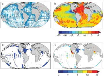
Fig. 1. (a)Locations of N∗data (all depths),(b)objectively mapped N∗(µM) for the depth interval 200–550 m,(c)locations ofδ15NO3 data (all depths), and(d)δ15NO3concentrations (‰) averaged over the depth interval 200–550 m.
effects of highly variable denitrification processes. Nitrate deficits can be measured by the N∗tracer, which reflects the difference between the in situ NO3 concentration and that
expected due to the average nitrate to phosphate (PO4) ratio
of organic matter, N∗= NO
3−16×PO4. The isotopic ratio
of15N to14N in oceanic nitrate (R=15NO3/14NO3) is
com-monly expressed as δ15NO3=(R/Rstd−1)×1000, where
Rstdis the isotopic ratio of atmospheric N2.
In tandem, N∗ andδ15NO
3 provide powerful constraints
on marine denitrification rates. Denitrification in both the wa-ter column and the sediments consumes nitrate but not phos-phate, imparting a negative signature to N∗. The influence of denitrification is clearly visible in the thermocline N∗ dis-tribution, which shows strongly negative N∗ due to water-column denitrification in suboxic waters of the Arabian Sea and the Eastern Tropical Pacific, and negative N∗ due to benthic denitrification in the sub-Arctic Pacific and else-where (Fig. 1b). Water-column denitrification preferentially removes the lighter nitrogen isotope, and imparts a heavy iso-topic signature ofǫw∼25‰ (Sigman et al., 2003) to
sur-rounding waters, which explains the elevatedδ15NO3values
in the suboxic waters of the eastern tropical Pacific and the Arabian Sea (Fig. 1d). However, benthic denitrification has a much lighter isotopic signature of 0‰≤ǫb.3‰ (Brandes
and Devol, 1997, 2002; Lehmann et al., 2004, 2007), as ev-idenced by the lack of isotopic enrichment in the sub-Arctic Pacific (e.g., Yoshikawa et al., 2006) (Fig. 1d).
The mean oceanδ15NO3of about 5‰ primarily reflects a
balance between the input of isotopically light NO3by
nitro-gen fixers (with an isotopic signature of−2‰.ǫfix≤0‰
(Macko et al., 1987; Carpenter et al., 1997)) and a mixture of water-column and benthic denitrification, and therefore pro-vides a strong constraint on the relative amounts of
denitrifi-cation occurring in the water column (W) and the sediments (B), which can be expressed compactly as the ratio B/W. Simple geochemical box models have been used to derive es-timates ofB/W, but these estimates still yield a large uncer-tainty of 1< B/W <4 (Brandes and Devol, 2002; Deutsch et al., 2004; Altabet, 2007; Eugster and Gruber, 2012). The uncertainty inB/Wpartly reflects uncertainty in isotopic en-richment factors and the isotopic ratio of organic nitrogen (Brandes and Devol, 2002; Altabet, 2007). More importantly however, the wide range of estimates of B/W reflects in-accuracies associated with simple box models, which can-not resolve important spatial features of the ocean circula-tion and denitrificacircula-tion processes. In order to correctly ac-count for the isotopic effects of nitrate consumption in the suboxic water column, a model should correctly simulate the degree of nitrate consumption in suboxic zones, and accu-rately simulate how the suboxic zones are ventilated and how tracers are exchanged between the suboxic and oxic ocean (e.g., Deutsch et al., 2004). These latter effects can only be accurately captured in a spatially explicit 3-D ocean circu-lation model. The only previous study to simulate nitrogen isotopes in a global ocean circulation model suffered from severe overconsumption of nitrate in the suboxic water col-umn (Somes et al., 2010), rendering theB/W estimate from that model inaccurate.
Here we address these issues by coupling a simple ni-trogen cycle model to a data-constrained ocean circulation model (Sect. 2.1). The parameters of the nitrogen cycle model are iteratively adjusted using an adjoint approach to achieve an optimal fit to the observed distributions of N∗ andδ15NO3(Sects. 2.2 and 2.3). The solution to this global
inverse nitrogen cycle model is an estimate of the global rates and patterns of water-column and benthic denitrification (Sect. 3). The effects of denitrification on the N∗distribution (Sect. 4.1) and on the mean oceanδ15NO3 (Sect. 4.2) are
discussed. Model parameters that are poorly constrained by the available data are varied by a Monte Carlo procedure in order to derive uncertainty estimates on denitrification rates (Sect. 4.3). We also discuss the implications of our findings for the global marine nitrogen budget (Sect. 5).
2 A global inverse nitrogen cycle model
2.1 Circulation model and nitrogen cycle model
phosphorus (DOP) cycle to the model, with the observed PO4
distribution (Garcia et al., 2010a) as an additional constraint on the circulation and biological fluxes. Unlike the study of DeVries et al. (2012), we do not assimilate CFC-11 (chlo-rofluorocarbon) observations in this version of the model.
The annual mean steady-state circulation determined in the above step is then taken offline and used to compute the physical tracer transport in a simple marine nitrogen cy-cle model. The internal cycling of N is driven by restor-ing surface nitrate toward observations, as done for PO4.
This ensures that the model reproduces the observed nutrient stoichiometry (N∗) of surface waters. One of the necessary chemical signatures of N2 fixation – a non-Redfield uptake
of NO3and PO4– is therefore already implicit in the model
design. Thus the N∗observations cannot simultaneously con-strain the rates and spatial distribution of N2fixation. Rather,
we model N2fixation according to a simple dependence on
light, temperature, and nutrient availability (see Appendix A), and use it primarily to close the N budget. An inverse solution that solves simultaneously for N2fixation and
deni-trification rates requires an explicit treatment of non-Redfield stoichiometry of nutrient uptake, as well as riverine and at-mospheric N inputs, and is left for a future study.
Water-column denitrification in the model occurs where observed oxygen concentrations fall below a critical thresh-old O2,crit. Observed oxygen concentrations are taken from
the 2009 World Ocean Atlas monthly climatology (Garcia et al., 2010b) after correcting for measurements in low-oxygen regions (Bianchi et al., 2012). Benthic denitrifica-tion occurs within grid cells that have some contact with the ocean floor. The grid cells having contact with the ocean floor are determined by interpolating observed bathymetry to the model grid, as described in Appendix A. Water-column den-itrification rates are proportional to the rate of organic matter remineralization within suboxic zones, while benthic deni-trification rates are proportional to the rate of organic matter supply to the sediments, and also depend on bottom-water ni-trate and oxygen concentrations. Denitrification in the water column and sediments is balanced by nitrogen fixation, with a rate that depends on local surface NO3concentrations,
tem-perature, light levels, and iron supply. Production of organic nitrogen is parameterized by restoring to observed NO3in the
top two model layers (above 73 m depth). Organic nitrogen is exported out of the surface layers as either dissolved organic nitrogen (DON) which remineralizes with first-order kinet-ics, or as particulate organic nitrogen (PON), which reminer-alizes according to a power-law dependence on depth (Mar-tin et al., 1987). See Appendix A for a full description of the nitrogen cycle model.
2.2 Inverse nitrogen cycle model
The parameters of the nitrogen cycle model include the crit-ical oxygen threshold for water-column denitrification; the ratio of nitrate consumed to organic matter remineralized
during water-column denitrification, and that during benthic denitrification; the oxygen and nitrate dependence of ben-thic denitrification; the isotopic enrichment factors for nitro-gen fixation, water-column denitrification, benthic denitrifi-cation, and uptake of nitrate to form organic nitrogen; the maximum nitrogen fixation rate as well as its temperature, light, nitrate, iron, and depth dependence; the fraction of or-ganic matter production routed to the dissolved oror-ganic ni-trogen (DON) pool; and the decay timescale for DON. Most of the model parameters can be constrained by the N∗ and
δ15NO3data, and these parameters (see Table B1) are
iter-atively adjusted using an adjoint method to find values that best fit observed N∗andδ15NO
3(Fig. 1). See Appendix B for
a full description of the inverse model and the formulation of the cost function measuring the model-data misfit.
We withhold four of the model parameters from the in-version because they are likely to be unconstrained by the available N∗andδ15NO
3data. Primarily due to the sparsity
of theδ15NO3observations, only one of the isotopic
enrich-ment factors can be constrained independently of the others. We solve forǫwas part of the solution to the inverse model,
since there is good data coverage in the suboxic zones where water-column denitrification occurs (Fig. 1c). We fix the iso-topic enrichment factor for uptake of nitrate to form organic matter (ǫup) at 5‰ as in previous studies (e.g., Somes et al.,
2010; Eugster and Gruber, 2012). We account for uncertainty in the remaining isotopic fractionation factors by rerunning the inverse model with various combinations ofǫb(0, 1, 2,
or 3‰) andǫfix (−2,−1, or 0 ‰). The fraction of organic
nitrogen routed to the DON pool (σDON) is also poorly
con-strained, since observations of DON concentrations are not used to constrain the model. So we also vary the value of
σDONover a wide range (σDON=1/4, 1/3, 1/2, or 2/3) in
dif-ferent versions of the inverse model. In all, the difdif-ferent com-binations ofǫw,ǫfix, andσDONproduce 48 configurations for
the inverse model. The uncertainty ranges quoted below rep-resent the full range of optimal model solutions under each of these 48 different model configurations.
Data constraints for the inverse model include N∗ con-centrations derived from the 2009 World Ocean Atlas ob-jectively mapped annual mean NO3 and PO4 data (Garcia
et al., 2010a), which are interpolated to the model grid, and
δ15NO3 observations compiled from the literature (Somes
et al., 2010; Rafter et al., 2012; De Pol Holz et al., 2009; Liu, 1979; DiFiore et al., 2009; Yoshikawa et al., 2005, 2006, P. Rafter and D. Sigman; and unpublished data), which are binned to the model grid. We excludeδ15NO3observations
above 200 m depth, due to numerical noise in the simulated
δ15NO3fields that can occur near the surface where nitrate
concentrations are very low (close to zero).
2.3 Model-data comparison
The optimization procedure produces a good fit to the ob-served distributions of N∗ (Fig. 2b) and δ15NO
0 10 20 30 40 50
0 10 20 30 40 50 -15 -10 -5 0 5
-15 -10 -5 0 5
4 8 12 16 20
0 0 4 8 12 16 20 -0.2 μM 1.4 μM RMSE
Mean -0.2 μM
1.2 μM RMSE Mean 0.0 ‰ 0.8 ‰ RMSE Mean
0.4 0.5 0.6 0.7 0.8
4 8 12 16 20 24 a b c d Modeled NO 3 (μM)
Observed NO3 (μM) Observed N* (μM)
Modeled N* (μM)
0.9
Observations
Model ETNPArabian Sea ETSP
NO3/(16*PO4)
δ 15NO 3 (‰) 0 10 20 30 40 50 60 70 80 90 100 Modeled δ 15NO 3 (‰)
Observed δ15NO 3 (‰)
(percentile)
Fig. 2. (a–c)Joint distribution function for the gridbox-volume-weighted observed and modeled tracer concentrations. The joint distribution function was estimated using the kernel density esti-mation method described in Botev et al. (2010), with a modification to account for the volume of the model grid boxes (Primeau et al., 2013). Printed on each plot is the gridbox-volume-weighted mean model-data difference and the gridbox-volume-weighted root mean squared error.(d)Modeled and observedδ15NO3vs. remaining ni-trate (1−fc) for all locations withδ15NO3observations and O2 concentrations less than 20 µM. Symbols in(d)distinguish differ-ent oceanic regions. Results plotted here are averages of the optimal solutions under all 48 different model configurations.
Although NO3is not included in the cost function
measur-ing model-data misfit, a good fit to observed NO3(Fig. 2a)
is achieved by virtue of the fact that both PO4 and N∗ are
included in the cost function. The mean modeled nitrate and N∗ concentrations are slightly lower than the observed values, and the mean oceanδ15NO3 is around 5 ‰, in
ex-cellent agreement with the observations. The model also demonstrates good agreement with the observed degree of ni-trate consumption (fc= 1–NO3/16PO4) andδ15NO3in
low-oxygen zones (Fig. 2d). The degree of nitrate consumption in waters with less than 20 µM O2 in the model is between
0.1–0.5, in agreement with observations. At high degrees of nitrate consumption (fc∼0.4), the modeledδ15NO3is about
12–16 ‰, depending on the oceanic region. This agrees with the mean observedδ15NO3in these regions, although the
ob-servations show more scatter than the modeled values. This could be due to spatial or temporal variability that is not cap-tured by the coarse steady-state model.
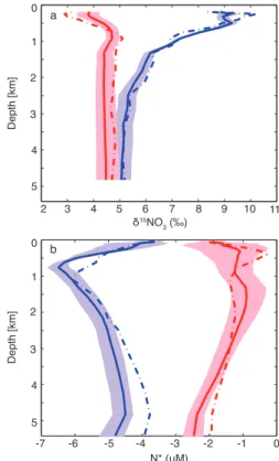
The model also matches the depth distribution of N∗ and δ15NO3 in both the Atlantic and Indo-Pacific basins
quite well (Fig. 3). Depth profiles of modeled and observed
δ15NO3 in the Atlantic show that the model does not
pro-Depth [km] 0 1 2 3 4 5
5 6 7 8 9 10
-4 -3 -2 δ15NO
3 (‰)
N* (μM) 11 4 3 2 -1 0 Depth [km] 0 1 2 3 4 5 a b -5 -6 -7
Fig. 3. (a)Depth profiles of modeled (solid curve) and observed (dashed curve) δ15NO3 for the Indo-Pacific (blue) and Atlantic (red) basins. Depth averages are taken over all model grid cells for which there is at least oneδ15NO3observation. There are no observations below 4800 m, and observations at depths shallower than 200 m are not used to constrain the model.(b) Depth pro-files of modeled and observed N∗for the Indo-Pacific and Atlantic basins. Shading around model mean depth profile is the range from all model solutions.
duce quite low enough δ15NO3 near the surface (Fig. 3a).
Atmospheric deposition, which is not accounted for in the model, may play an important role in determining the shal-low nitrateδ15NO3in the Atlantic (Knapp et al., 2008). Deep
ocean values in the Atlantic are slightly lower than observed, but the observations lie within the envelope of model uncer-tainty. The modeled depth profile of δ15NO3 in the
Indo-Pacific basin matches the observations fairly well through-out the water column (Fig. 3a). The greatest mismatch oc-curs above 500 m, where modeledδ15NO3is lower than
ob-served. This could potentially indicate too little N fixation in the model in regions withδ15NO3 observations,
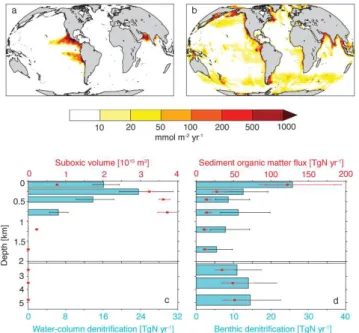
Fig. 4. (a)Depth-integrated rate of water-column denitrification,
(b)depth-integrated rate of benthic denitrification,(c)water-column denitrification rate (blue bars with black error bars, lower axis) and suboxic volume (red circles with red error bars, upper axis) in-tegrated over various depth intervals (0–160 m, 160–350 m, 350– 550 m, 550–1000 m, 1000–1400 m, 1400– 2000 m, 2000–3000 m, 3000–4000 m, and 4000–5500 m) and (d) benthic denitrification rate (blue bars with black error bars, lower axis) and sediment or-ganic matter flux rate (red circles with red error bars, upper axis) integrated over the same depth intervals as in(c). Note nonlinear color scale in(a)and(b). Vertical axis stretched for top 2000 m in
(c)and(d). Median rates are given in(a)and(b), while error bars in(c)and(d)span the full range of model predictions.
N∗ depth profile in the Indo-Pacific, with some distinctive differences most notably in the depth range 500–1000 m where the model has a stronger and shallower negative N∗ peak than the observations, and in the deep ocean where the model N∗is more negative than observed (Fig. 3b). However, the largest model-data misfit (∼1 µM) is small compared to the N∗signature of denitrification (see for example Fig. 5a and discussion below).
3 Denitrification rates and their global distribution
The global distribution of water-column and benthic denitri-fication (Fig. 4) was determined from the optimal solution under each of the 48 different model configurations. Water-column denitrification best fits observations when confined primarily to low-oxygen zones (O2.5 µM) in the eastern
tropical North and South Pacific, and in the Arabian Sea (Fig. 4a). Small (negligible) amounts of water-column den-itrification occur in the sub-Arctic Pacific and in the Bay of Bengal. Globally, the rate of water-column denitrification
N* due to denitrification (μM)
r N:P
Depth (km)
modeled N:P corrected for denitrification −5 −4 −3 −2 −1 0
5 10 15 20 25
a
4 3 2 1
Depth (km)
4 3 2 1
benthic
water column
b
Fig. 5. (a)The depth distribution of N∗due to benthic denitrification
(filled magenta circles with error bars) and water-column denitrifi-cation (open black circles with error bars).(b)The N : P ratio of remineralized organic matter calculated according to the method of Anderson and Sarmiento (1994) using the modeled NO3and PO4 fields (red circles with error bars), and the ratio after correcting for the amount of NO3that is lost due to denitrification (black circles with error bars). All calculations are performed on isopycnal sur-faces and plotted at the mean depth of each isopycnal.
predicted by the model is 50–77 Tg N yr−1(Table 1). Of this total, 9–14 Tg N yr−1is due to denitrification in the Arabian Sea, and 41–63 Tg N yr−1is due to denitrification in the east-ern tropical Pacific (Table 1). These rates agree, within their uncertainty, with an independent estimate of fixed nitrogen loss rates based on N2 gas observations from within these
same suboxic zones (DeVries et al., 2012). This agreement occurs despite the fact that the present study does not explic-itly account for fixed nitrogen loss due to anaerobic ammo-nium oxidation (anammox), while the estimate of DeVries et al. (2012) does implicitly include the effects of annamox. This agreement indicates that either anammox is similar to traditional denitrification in its imprint on N∗andδ15NO3, or
that annamox represents a small sink of fixed nitrogen within suboxic zones.
of shallow continental shelves (e.g., the sub-Arctic Pacific, northeast North America, Indonesian Archipelago, Arctic margin, and southeastern South America) (Fig. 4b). These areas experience benthic denitrification rates over 100 times greater than rates typical of deep ocean sediments. Globally, the model predicts that 70–170 Tg N yr−1of benthic denitri-fication is needed to match the constraints provided by the N∗andδ15NO3data, with the largest contribution from
sed-iments in the Pacific Ocean (Table 1).
The vertical distribution of water-column denitrification is highly concentrated and confined above 1000 m depth, co-incident with the depth of suboxic zones (Fig. 4c). Water-column denitrification rates have a shallower peak than the suboxic volume (Fig. 4c) due to the fact that organic mat-ter remineralization rates decrease with depth. Benthic den-itrification also has a shallow peak, with highest rates above 1000 m depth, although approximately half of benthic deni-trification occurs below 1000 m (Fig. 4d). The primary factor controlling the distribution of benthic denitrification is the rate at which organic matter is delivered to the sediments. However, the data imply a mid-depth peak in benthic denitri-fication at about 1000–2000 m that is not found in the rate of organic matter supply to the sediments (Fig. 4d), which the model ascribes to enhanced benthic denitrification rates un-der low oxygen and high nitrate conditions (e.g., Middelburg et al., 1996; Bohlen et al., 2012).
The rates of benthic denitrification reported here are lower than some earlier estimates, which were on the order of ∼250–300 Tg N yr−1 (Middelburg et al., 1996; Seitzinger
et al., 2006). However, more recent estimates are in better agreement with the benthic denitrification rates derived here. Bianchi et al. (2012) used the meta-model parameterization of Middelburg et al. (1996) and satellite-derived estimates of sinking organic matter flux to infer a benthic denitrification rate of 182±55 Tg N yr−1, while Bohlen et al. (2012) de-rived data-based transfer functions to scale satellite-dede-rived estimates of sinking organic matter flux to estimates of ben-thic denitrification, arriving at a globally integrated benben-thic denitrification rate of ∼155 Tg N yr−1. These more recent estimates agree within uncertainty with the benthic denitrifi-cation rate found in this study (70–170 Tg N yr−1), although
our estimate is, on average, slightly lower.
A significant difference between this study and previous studies is that our model predicts that only about 20 % of benthic denitrification occurs in shelf sediments (<160 m depth), in contrast with other estimates suggesting 35–70 % of benthic denitrification occurs on continental shelves (Mid-delburg et al., 1996; Bianchi et al., 2012; Bohlen et al., 2012). Although we have used a parameterization to account for the presence of shallower continental shelves than are re-solved by the model’s bottom topography (see Appendix A), the model resolution is still insufficient to resolve the en-hanced biological productivity and high organic carbon ex-port rates within shelf regions. Because the model underes-timates benthic denitrification on continental shelves, and in
order to maintain the correct ratio of benthic to water-column denitrification, the model probably slightly overpredicts the amount of denitrification in the deep ocean. That there is too much benthic denitrification in deep sediments can be seen in Fig. 3, which shows that model-predicted N∗is about 20 % lower than observed in the deep ocean. If denitrification in shelf areas produces less of an imprint on the mean ocean
δ15NO3than denitrification in deep sea sediments, this could
produce a slightly low bias in the total benthic denitrification rate found by the model.
A further consideration is that riverine N sources are ig-nored in the model. An additional input of nitrate to the con-tinental shelf areas could be supplied by rivers, which are estimated to deliver about 30 Tg N yr−1 into coastal waters
(Gruber and Galloway, 2008), with an isotopic enrichment of about 4 ‰ (Brandes and Devol, 2002). If this were balanced entirely by denitrification on the shelf areas, this would also serve to increase the proportion of benthic denitrification oc-curring on continental shelves.
4 Discussion
4.1 Effect of denitrification on vertical N∗distribution
Water-column and benthic denitrification have distinct ef-fects on the vertical distribution of N∗ in the ocean. Quan-tifying these effects can help to reveal the imprint of water-column and benthic denitrification on N∗, and allow us to judge the relative misfit between the modeled and observed N∗depth profiles (Fig. 3). To estimate the effect of denitrifi-cation on N∗, we simulate an idealized denitrification tracer that is produced at a rate of 1 mol tracer per 1 mol NO3
consumed by denitrification. The tracer is immediately re-moved from the ocean when it reaches the top model layer, where all nutrients are considered “preformed”. We perform separate calculations for benthic and water-column denitri-fication. For comparison with the study of Anderson and Sarmiento (1994), we calculate the average amount of tracer on isopycnal horizons (below 400 m depth) and plot the re-sults as a function of the average depth of each isopycnal horizon (Fig. 5a). The results show that N∗ due to water-column denitrification reaches a minimum in the thermo-cline at about 700–800 m depth, with a peak value of around −1 µM (Fig. 5a). Benthic denitrification produces an N∗ pro-file with a mid-depth peak of about−3 to−4 µM at 1500– 3000 m depth (Fig. 5a). These are the globally averaged ef-fects of denitrification; the effect is about 50 % larger in the Indo-Pacific Basin, where most denitrification occurs and where waters are older, allowing for accumulation of reac-tion products. From this calculareac-tion, we see that the misfit between modeled and observed N∗depth profiles (Fig. 3b) is relatively small compared to the denitrification signal.
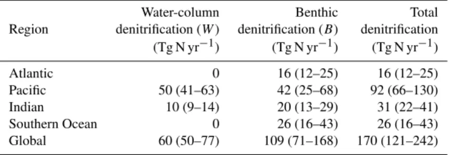
Table 1.Integrated denitrification rates by ocean basin. Median rate is given, with range in parentheses. The range includes uncertainty due to uncertainty in the isotopic enrichment factors of fixation and benthic denitrification, and in the parameterization of dissolved organic matter. Southern Ocean is south of 34◦S. Global rates also include contribution from benthic denitrification in the Arctic Ocean and the Mediterranean Sea.
Water-column Benthic Total
Region denitrification (W) denitrification (B) denitrification (Tg N yr−1) (Tg N yr−1) (Tg N yr−1)
Atlantic 0 16 (12–25) 16 (12–25)
Pacific 50 (41–63) 42 (25–68) 92 (66–130)
Indian 10 (9–14) 20 (13–29) 31 (22–41)
Southern Ocean 0 26 (16–43) 26 (16–43)
Global 60 (50–77) 109 (71–168) 170 (121–242)
accounted for when determining N : P ratios of regenerated organic matter from subsurface nutrient concentrations. We calculated the N : P ratio of remineralized organic matter in the interior ocean in our model following a procedure sim-ilar to that of Anderson and Sarmiento (1994). The amount of “preformed” nitrate (or phosphate) in the interior ocean is calculated from an idealized tracer with a surface concen-tration equal to the modeled surface concenconcen-tration, and no sources or sinks in the interior ocean. The amount of reminer-alized nitrate (or phosphate) is then determined by subtract-ing the preformed component from the total concentration. We determine the N : P ratio of remineralized organic matter from a linear regression of remineralized nitrate against rem-ineralized phosphate along the same isopycnal horizons used in Fig. 5a. Similar to the results of Anderson and Sarmiento (1994), we see that the near-surface N : P ratio calculated in this way is close to that of “fresh” organic matter (∼16:1), but drops to a minimum in the depth range 1500–3000 m (Fig. 5b). Anderson and Sarmiento (1994) hypothesized that the actual N : P ratio of remineralized organic matter was ap-proximately constant with depth, but that the mid-depth min-imum may be an artifact of benthic denitrification. By adding back in the remineralized NO3that is lost due to
denitrifica-tion (Fig. 5a) and repeating the calculadenitrifica-tion, we find that in-deed the N : P ratio of remineralization is approximately con-stant with depth (Fig. 5b), which is consistent with the origi-nal hypothesis of Anderson and Sarmiento (1994). The deep-est isopycnals in Fig. 5b are associated with deep Labrador Sea water in the western North Atlantic, a small region in which production is clearly non-Redfieldian.
4.2 Controls on the partitioning between benthic and
water-column denitrification
We find a median value ofB/W=1.7 in our suite of opti-mized models, with a range of 1.3< B/W <2.3. This sig-nificantly reduces the uncertainty on B/W over that de-rived from geochemical box models, which gave a range of 1< B/W <4 (Brandes and Devol, 2002; Deutsch et al.,
2004; Altabet, 2007). The relatively low value ofB/W deter-mined in this study contrasts with results expected from a lin-ear isotope mass balance model (Brandes and Devol, 2002), which predicts the following relationship forB/W,
B W =
ǫw−δ+ǫfix
δ−ǫfix−ǫb
, (1)
whereδ≈5‰ is the mean nitrogen isotopic ratio of oceanic nitrate, and a balance between inputs by nitrogen fixation and removal by benthic and water-column denitrification is assumed. If both ǫfix=0‰ and ǫb=0‰, Eq. (1) predicts
B/W=4. However, the global inverse model predicts that
B/W is about 1.9 in this case. This is because the impact of isotopic fractionation associated with water-column denitri-fication is diminished by the degree of nitrate consumption in suboxic zones (Deutsch et al., 2004). We find that the mod-eledB/W ratio can be well predicted (Fig. 6) by applying a simple correction to Eq. (1) to account for the degree of nitrate consumption (fc) in suboxic zones
B W =
(1−fc)ǫw−δ+ǫfix
δ−ǫfix−ǫb
. (2)
To apply Eq. (2) to our model results, we calculate fc
as the average of 1 – NO3/16PO4 in the core of the
sub-oxic zones (where observed O2 is less than O2,crit), and
δ=(15NO
3/NO3−1)×1000, where the bar indicates the
whole ocean average. For the model, we getδ=5.4‰ (range 5.2–5.7 ‰) andfc=0.34 (range 0.32–0.37).
This predictive relationship suggests that if there is com-plete consumption of nitrate in suboxic zones (fc=1), then
the isotopic enrichment effect of water-column denitrifica-tion does not affect the mean ocean δ15NO3. In fact, the
full effect of the isotopic enrichment due to water-column denitrification can never be achieved, becausefc>0
when-ever there is any water-column denitrification. In the model, the average fc within suboxic zones of about 0.34
Modeled B/W Equation (1)
1.4 1.6 1.8 2.0 2.2
Predicted B/W
1 2 3 4
5 Equation (2)
1:1 line
Fig. 6.Modeled ratio of benthic to water-column denitrification (B/W) compared to that predicted by a linear isotope mass balance (Eq. 1, bold red circles) and an isotope mass balance corrected for the fractional consumption of nitrate in suboxic zones (Eq. 2, bold blue circles). The faint dashed blue circles show results from equa-tion (2) when the mean oceanδ15NO3is corrected for fractionation during uptake of nitrate to form organic matter.
fc in suboxic zones agrees well with the observed average
fc=0.31 within those same locations.
Equation (2) slightly overpredictsB/W by about 0.15, on average, primarily because Eq. (2) does not take into account the isotopic enrichment during the assimilation of nitrate to form organic matter. To obtain the magnitude of this effect we re-ran the model withǫup=0‰ and all other parameters
fixed at their values determined by the inversion process. The results show that the fractionation associated with nitrate as-similation lowers the mean oceanδ15NO3 by about 0.5 ‰,
on average (minimum of 0.3 ‰ and maximum of 1.2‰ in all the model runs). Taking uptake fractionation into account, by replacingδ in Eq. (2) by the value ofδ in the case that
ǫup=0‰, leads to a prediction that slightly underestimates
the modeledB/W by about 0.15, on average. Equation (2) is therefore accurate within about±0.15, depending on the value ofǫupand on the actual value ofB/W. Remaining
dis-crepancies between the value ofB/W predicted by Eq. (2) and that determined by the model are likely due to the inade-quacy of using a single value offcto account for the spatially
heterogeneous effects of water-column denitrification. These results emphasize the importance of simultaneously achieving good fits to both nitrate deficits (to getfccorrect)
and nitrogen isotopes (to get δ correct) in order to derive a good estimate of marine denitrification rates. Using only one or the other constraint can produce misleading results. For example, a box model that was tuned to fit mean ocean
δ15NO3but not N∗found a value ofB/W∼4 (Brandes and
Devol, 2002) because it did not take into account the effects of nitrate consumption in suboxic zones, while an ocean
cir-εb
εfix
εfix
εb
0 1 2 3
0 -1 -2
0 1 2 3
0 -1 -2
150 160
1.8
1.9 2.0
170 180
190 200
1.7 1.6
1/4 1/3 1/2 2/3 1/4 1/3 1/2 2/3
Fraction of production to DON (σDON)
0 50 100 150 200 250
T
otal denitirification [TgN yr
-1]
0 0.5 1.0 1.5 2.0 2.5
B/W
a b
c d
Fraction of production to DON (σDON)
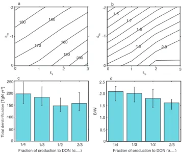
Fig. 7. (a)Globally integrated denitrification (Tg N yr−1) and(b)
ratio of benthic (B) to water-column (W) denitrification as a func-tion of isotopic enrichment factors for nitrogen fixafunc-tion (ǫfix) and benthic denitrification (ǫb).(c)Globally integrated denitrification and(d)B/Was a function of the fraction of organic matter produc-tion routed to the dissolved organic nitrogen (DON) pool. Results in
(a)and(b)show mean values from all model solutions, and results in(c)and(d)show median (filled bars) and range (error bars) from all model solutions.
culation model that was tuned to fit mean oceanδ15NO3but
not N∗ found a value ofB/W∼0.5 (Somes et al., 2010), because the modeledfcwas too large.
To reduce the uncertainty on the exact value of B/W
will require more accurate knowledge of the isotopic enrich-ments factors for nitrogen fixation (ǫfix), benthic
denitrifi-cation (ǫb), and water-column denitrification (ǫw).
Labora-tory experiments with denitrifying bacteria have found val-ues forǫw as high as 30‰ (Barford et al., 1999) or as low
as 10–15 ‰ (Kritee et al., 2012). In our model, the opti-mal value of ǫw depends on the values ofǫfix andǫb, and
ranges from 19–29 ‰ throughout our suite of model config-urations. The lower values of ǫw are associated with high
values ofǫb andǫfix. Ifǫbwere as high as 4–5 ‰, as
sug-gested by some measurements (Alkhatib et al., 2012), then the optimal value of ǫw would approach the lower values
suggested by Kritee et al. (2012).
It is interesting to compare our results to those from a conceptually similar study that systematically tuned the pa-rameters of a multibox ocean model to fit observed N∗ and mean ocean δ15NO3 (Eugster and Gruber, 2012). The
two studies arrive at similar overall denitrification rates (107–188 Tg N yr−1in Eugster and Gruber (2012) compared to 120–240 Tg N yr−1 in this study) and B/W (1.6–2.0 in Eugster and Gruber (2012), 1.3–2.3 in this study). The agree-ment between the box model and our results in terms ofB/W
B/W
Relative model-data misfit
1 10 100
1 1.5 2 2.5
N* with isotope constraint N* no isotope constraint δ15NO3 with isotope constraint
δ15NO3 no isotope constraint
Fig. 8.Sensitivity of model-data misfit to partitioning of denitrifica-tion between sediments and water column. We start with a model so-lution in which only N∗is used as a constraint (open symbols), and one in which both N∗andδ15NO3are used as constraints (closed symbols). We then varyB/Wby adjusting the parameters determin-ing the rate of benthic denitrification, while keepdetermin-ing all other param-eters and the total denitrification rate constant. These experiments use the model configuration withǫfix=0,ǫb=0, andσDON=1/4.
ocean δ15NO3 and the fractional consumption in suboxic
zones (Eq. 2), and that details of the ocean circulation are probably a second order influence on B/W. However, the total rate of denitrification is likely to be more sensitive to details of the ocean circulation, which influences the pattern and magnitude of biological production, the extent of sub-oxic zones, and the spatial distribution of remineralization. Therefore, the agreement between the box model and our study in this regard may be partly fortuitous.
4.3 Uncertainty in denitrification rates
The globally integrated rate of marine denitrification pre-dicted by the model ranges from about 120–240 Tg N yr−1, with a median rate of 170 Tg N yr−1(Table 1). We find that
uncertainty in the isotopic enrichment factors (ǫfix andǫb)
and uncertainty in the fraction of organic matter production routed to the DON pool (σDON) contribute approximately
equally to the uncertainty in the globally integrated denitri-fication rate (Fig. 7a and c). Denitridenitri-fication rates generally increase with larger values ofǫbandǫfix(Fig. 7a). This
re-lationship follows because for larger values ofǫbor ǫfix, a
largerB/Wratio is needed to achieve a mean oceanδ15NO3
of ∼5‰ (Fig. 7b), which is achieved in the model by in-creasing benthic denitrification rates. It is also the case that
B/W increases with smallerσDON values (Fig. 7d). This is because with smallerσDONvalues a larger fraction of
partic-ulate organic matter sinks out of the euphotic zone, yielding a larger supply of organic matter to the sediments.
The ratioB/Wis relatively well constrained despite large uncertainties in the isotopic enrichment factors. This is be-cause in the inverse model, the fractional consumption fc
in suboxic zones generally increases slightly with increasing values ofǫborǫfix, whileǫwdecreases with increasing
val-ues ofǫborǫfix. Both of these effects reduce the sensitivity
ofB/W to the isotopic enrichment factors for fixation and benthic denitrification.
The effects of the N∗andδ15NO3constraints on the ratio
ofB/W predicted by the model can be illustrated by com-paring the relative model-data misfit for each observational constraint as a function ofB/W. The results for one particu-lar model configuration show that the value ofB/W needed to optimally match only the observed N∗is about 1.4, while that needed to optimally match only the observedδ15NO3is
about 2.3 (Fig. 8). When both constraints are used, the model strikes a compromise between the two constraints such that the optimal value ofB/W is about 1.8 (Fig. 8). In this partic-ular model configuration, N∗provides the stronger constraint onB/W, as evidenced by the deeper minimum associated with the relative model-data misfit. This is owing to both the larger number of N∗observations compared toδ15NO3
ob-servations, and the fact that N∗ generally shows a stronger sensitivity to changes inB/W (holding all other model pa-rameters fixed) than doesδ15NO3.
The fact that the N∗ andδ15NO
3 constraints require
dif-ferent optimal B/W values is not surprising, given uncer-tainties in the model parameters and imperfections inherent in representing complex phenomena with simple parametric equations, as well as uncertainties in the data. Only with per-fect data and a perper-fect model could we expect the model to match both data sets optimally with the same set of param-eters. This further illustrates the importance of bringing to-gether both the N∗ andδ15NO3data as constraints on
deni-trification rates, as long as one deals with imperfect models and imperfect data. Furthermore, the advantage of the inverse model is that uncertainties are explicitly coded into the model in terms of the adjustable control parameters, and the model is given freedom to choose between different parameter val-ues in order to optimally match the observed N∗andδ15NO3.
5 Implications and conclusions
Results of our global 3-D inverse model simulations sug-gest that the optimal rate of water-column denitrification needed to match the observed N∗ andδ15NO
3 is about 60
(range of 50–77) Tg N yr−1, in good agreement with a pre-vious estimate based on N2 gas measurements (DeVries
et al., 2012). Meanwhile, the optimal value of B/W is about 1.7 (range 1.3–2.3). These estimates represent a sig-nificant improvement over previous estimates from box mod-els (Brandes and Devol, 2002; Deutsch et al., 2004; Altabet, 2007; Eugster and Gruber, 2012), which could not resolve the 3-D ocean circulation and the full spatial variability in denitrification rates.
While the denitrification rates estimated here significantly reduce the uncertainty on the global rate of fixed N loss from the ocean, some significant uncertainties in the marine N cycle remain that cannot be addressed using the present model. Perhaps most importantly, we have not addressed the magnitude and distribution of N2 fixation rates. A
model-ing study that used surface N∗ distributions to estimate ni-trogen fixation rates found a global N2fixation rate of about
140 Tg N yr−1 (Deutsch et al., 2007), while a recent obser-vational study suggests that the global rate of N2 fixation
is about 180 Tg N yr−1 (Grosskopf et al., 2012), which is approximately equal to the mean global denitrification rate found in this study. However, it is not known precisely what amount of fixation is supported by the N∗andδ15NO
3data
in our model. This is because the information contained in the surface N∗ distribution, which can in principle be used to constrain rates and patterns of nitrogen fixation (e.g., Deutsch et al., 2007), has already been absorbed by the sur-face restoring condition used to simulate the production of organic phosphorus and organic nitrogen.
Similarly, we have not explicitly considered sources of N due to riverine inputs and atmospheric deposition, which could have significant local impacts on surface N∗ and
δ15NO3distributions (e.g., Hansell et al., 2007; Knapp et al.,
2008). However, whatever spatial pattern these fluxes impart to N∗in surface waters is achieved by restoring toward ob-served NO3and PO4independently, and their effect on the
N reservoir will be implicitly included in our “N2fixation”
term. In the case of isotopic constraints, the effect of these surface fluxes is not similarly accounted for, but if the iso-topic signature of those fluxes is on balance not significantly different from that of N2fixation (e.g., Brandes and Devol,
2002) then these inputs could again be considered part of the “N fixation” term that closes the budget. Given the uncer-tainty surrounding the isotopic ratio of these N inputs, this assumption must be taken as provisional. Lastly, some esti-mates suggest that human activities may have more than dou-bled riverine and atmospheric N inputs from their preindus-trial values (Gruber and Galloway, 2008). The effect of these anthropogenic perturbations on nutrient distributions and on denitrification rates is poorly known, but should be addressed in future studies.
Appendix A
Nitrogen cycle model description
The governing equations for nitrate (NO3) and dissolved
or-ganic nitrogen (DON) are ∂NO3
∂t =ANO3−Jprod+J
wc
rem+Jremsed+JfixNO3−Jwcd−Jsd+ 1
τDON
DON, (A1) ∂DON
∂t =
A− 1 τDON
DON+σDONJprod+JfixDON, (A2)
where the linear operator A represents the model’s dis-cretized advection-diffusion transport operator, andτDONis
a decay timescale for DON. The other sources and sinks are nonlinear and are described below.
Production of organic nitrogen (Jprod) in the euphotic zone
represents a sink of nitrate and is parameterized by restoring to mean annual observed NO3 (Garcia et al., 2010a) above
zc= −73 m (corresponding to the top two model layers) with
a restoring timescaleτb=30 days:
Jprod(x, y, z)=
1
τb
(NO3−NO3,obs),NO3>NO3,obs (A3)
Jprod(x, y, z)=0,NO3≤NO3,obs, z < zc. (A4)
Of the total production of organic N, a fractionσDONis
routed to the DON pool, and the remainder (1−σDON) to
particulate organic nitrogen (PON). PON is remineralized in the water column with a vertical attenuation described by a power-law flux profile (Martin et al., 1987):
Jremwc(x, y, z)= ∂
∂z
(1−σDON) zc
Z
0
Jprod(x, y, z)dz z
zc −b
. (A5)
Whatever PON is not remineralized in the water column is remineralized in the sediments (Jremsed) within that same ver-tical column. In the process of generating the coarse model grid, many areas that would normally be partially covered by land or have some sediment interface, such as continental shelves and islands, are completely covered over in water. We use a parameterization to account for these areas, so that rem-ineralization in the sediments occurs not only in the last wet grid cell in each vertical column, but is distributed within the column in accordance with the fraction of each grid cell that is covered by a shallower land area. This fraction is deter-mined by interpolating a high resolution bottom topography (ETOPO2v2) to the model grid.
Like production, nitrogen fixation occurs in the top two model layers. The local nitrogen fixation rate is given by
Jfix=Fo×e−NO3/λ×e(T−Tmax)/To× I I+KI
× Fe
Fe+KFe, (A6)
for warm seawater temperatures (T) and adequate light (I) and iron (Fe) supply (e.g., Monteiro et al., 2011).Tmaxis the
maximum modeled surface temperature (about 31◦C), which is included to ensure that the maximum of the exponential ex-pression in equation (A6) is 1. Iron is not modeled explicitly, but rather we use a modeled dust deposition field (Mahowald et al., 2006) as a proxy for its availability (e.g., Somes et al., 2010). The surface irradianceI is derived from International Satellite Cloud Climatology Project-C1 data (Zhang et al., 2004). The environmental controls in equation (A6) help the model to reduce N2fixation in places where rates are known
to be low, such as the Southern Ocean.
Of all the newly fixed organic matter, a fraction φe is routed to the PON pool and remineralizes in the water-column (Jfixwc) and sediments (Jfixsed), following the same formulation as regular organic matter (Eq. A5). Another fractionφd=φe×σDON/(1−σDON)is routed to the DON
pool (JfixDON) and remineralizes following the first-order ki-netics for DON remineralization. The remaining fraction (1−φe−φd) remineralizes immediately in the surface layers where fixation occurs. Thus, the individual fixation terms in Eqs. (A1) and (A2) are
JNO3
fix =(1−φe−φd) Jfix, z≥zc, (A7)
JNO3
fix = Jfixwc+Jfixsed, z < zc, (A8)
JfixDON= φdJfix, z≥zc. (A9)
Denitrification in the water column occurs wherever lo-cal observed O2 levels fall below a critical level (O2, crit)
representing the threshold at which denitrification re-places oxic respiration as the dominant pathway of organic matter degradation:
Jwcd=rNdenit:Norg×(J wc
rem+Jfixwc+
1
τDON
DON) (A10)
⇐⇒ O2,obs<O2,crit
where rNdenit:Norg represents the ratio of moles NO3 used
to respire 1 mol of organic nitrogen. The “if and only if” ⇐⇒ statement is handled by creating a mask from ob-served monthly climatology of oxygen concentrations (Gar-cia et al., 2010b) after applying the correction suggested by Bianchi et al. (2012) using the procedure described by DeVries et al. (2012).
Benthic denitrification is parameterized as a function of the rate of organic matter respiration in the sediments:
Jsd=F×(Jremsed+Jfixsed) (A11)
whereF is a function that accounts for enhanced sedimen-tary denitrification rates under low-oxygen and high-nitrate
conditions,
F =a0+a1FO2+a2FNO3+a3FO2FNO3, (A12)
FO2 =tanh
C
O2−O2
KO2
+1, (A13)
FNO3 =
NO3
NO3+KNO3
, (A14)
where CO2, KO2 and KNO3 are parameters governing the
oxygen and nitrate dependence of sedimentary denitrifica-tion. A hyperbolic tangent was chosen for the O2dependence
of benthic denitrification to allow for uncertainty in how the transition to O2-inhibition takes place (i.e., it can be either
an abrupt or a smooth transition). Ultimately, we found the parameter controlling the smoothness of the transition (KO2)
to be poorly constrained (see Table B1). The linear depen-dence of benthic denitrification on sediment organic matter flux (Eq. A11) was chosen because of its simplicity and ease of implementation in the model. By contrast, Middelburg et al. (1996) suggest a nonlinear relationship between benthic denitrification and organic matter fluxes. However, we found that our linear formulation produces similar overall rates and spatial patterns to the Middelburg et al. (1996) formulation. We also tested a version in which benthic denitrification de-pended quadratically on sedimentary organic matter fluxes, and found no improvement over the linear model.
The coupled system of nonlinear equations (Eqs. A1– A2) for NO3and DON are solved using Newton’s method,
which produces convergence to an equilibrium state orders of magnitude faster than traditional time-stepping techniques (Kwon and Primeau, 2006). Fast convergence to an equi-librium solution is necessary for application in the inverse model, which requiresO(103) runs of the forward model to
converge to a solution.
The governing equations for 15NO3 and DO15N are the
same as Eqs. (A1) and (A2) except that a fractionation fac-torαrepresenting the discrimination of chemical reactions toward the lighter isotope is introduced in each term that in-volves a chemical reaction (e.g., Deutsch et al., 2004). Gener-ically, the reaction rate (Jreac) for15N is related to the
reac-tion rate for14N by
J15N O3
reac =α
15NO 3 14NO
3
J14NO3
reac (A15)
This fractionation effect is taken into account in the uptake of NO3 to form organic N (Jprod), the remineralization of
organic N by denitrifying bacteria in the water column (Jwcd)
and the sediments (Jsd), and the fixation of atmospheric N2
(Jfix). The isotopic enrichment factor for a reaction is given
byǫ=(1−α)×1000.
Given the steady-state solution for NO3and DON obtained
from solving Eqs. (A1) and (A2), and making the approxi-mation14NO3≡NO3and DO14N≡DON, the equations for 15NO
system of equations for the isotopic ratios:
RNO3 = 15NO
3/14NO3
Rstd
, (A16)
RDON=
DO15N/DO14N
Rstd
, (A17)
whereRstdis the isotopic ratio of atmospheric N2, which we
take to be 1 for convenience. The resulting set of coupled linear equations can be solved by direct matrix inversion. In places where NO3concentrations are very low (close to zero)
we find that the ratioRNO3can become ill-defined, leading to
noise in the model-simulatedRNO3 distribution. For this
rea-son, we neglectRNO3 values above 200 m depth, where very
low NO3can occur, when comparing the modeled and
ob-servedδ15NO3values in the inverse model (see below). We
find that a similar problem occurs where DON concentrations are close to zero, which occurs in many places in the inte-rior ocean. These points can cause an ill-conditioned (nearly singular) matrix when inverting for the modeledRNO3 and
RDONvalues. We find that this problem is eliminated when
we set all values where DON< γ toγ, whereγ is a small number (we used 10−4µM). This does not affect the
mod-eledRNO3 values.
When comparing modeled to observed isotopic ratios for NO3, we convert observedδ15NO3 values to RNO3 values
using the relationshipδ15NO3=(RNO3−1)×1000.
Appendix B
Inverse model description
The procedure by which the model is fit to observed N∗and
δ15NO3involves two steps. In the first step, the model
circu-lation and air–sea fluxes are adjusted to minimize the misfit between modeled and observed temperature, salinity, radio-carbon, and phosphate distributions. This procedure follows that outlined in DeVries and Primeau (2011), except that here we use a higher resolution model grid (2◦ horizontal reso-lution with 24 unevenly spaced vertical levels) and we in-clude phosphate observations from the 2009 World Ocean Atlasgridded database (Garcia et al., 2010a) in the set of ob-servations constraining the model. The cycling of phosphate and dissolved organic phosphorus (DOP) are both explicitly modeled, following the same sets of equations described for the nitrogen cycle, except that the fixation and denitrification terms are of course not included. We include the depth atten-uation coefficientbfor particulate organic phosphate (POP) remineralization as an additional control parameter of the model to be determined as part of the optimization. Two addi-tional parameters,σDOPandτDOPare needed for the model,
but these cannot be determined as part of the optimization because DOP data is not included in the set of observational constraints. Rather, we specifyσDOPandτDOPbased on
val-ues determined in previous studies. In one model we specify
σDOP=2/3 andτDOP=1/2 yr (Najjar and Orr, 1998), and
in another model we specifyσDOP=1/2 and τDOP =2 yr (Schlitzer, 2002).
The relative error of model state variables in this first step of the optimization is 0.8 for temperature, 0.8 for salin-ity, 0.65 for114C, and 0.75 for phosphate in the case that
σ=1/2 andτDOP=2 yr (0.78 in the case that σDOP=2/3
andτDOP=1/2 yr). Relative errors of about 1 indicate that
the model-data residuals are distributed according to the prior estimated error covariance for the global gridded data sets (cf. DeVries and Primeau, 2011). Primarily due to computa-tional restrictions, we did not use CFC observations to con-strain the circulation, unlike a previous study (DeVries et al., 2012). When compared to observed CFC concentrations, the model does show some deficiencies in ventilating the sub-oxic zones. In particular, the Arabian Sea subsub-oxic zone is apparently too weakly ventilated near the surface and too well ventilated at depth, while the eastern tropical South Pa-cific is too well ventilated throughout. In the future it will be important to assimilate CFC observations into the model to reduce these circulation errors. Despite this, we find that at the global scale the water-column denitrification rates de-rived here (50–77 Tg N yr−1) are similar to those derived by DeVries et al. (2012) (66±6 Tg N yr−1) using a model that was constrained by CFCs and that used N2/Ar observations
to constrain denitrification rates. This indicates that circula-tion errors within the suboxic zones are small enough not to have a large impact on the globally integrated water-column denitrification rates.
The circulation found in step one of the optimization is then taken offline and used in the nitrogen cycle simula-tion. Most of the parameters of the nitrogen cycle model (Eqs. A1–A17) are included as control parameters in this second step of the inversion (Table B1). One important ex-ception is that we fix the depth attenuation coefficient for PON remineralization (b) at the value found in step one of the inversion. The value of b determined from step one of the inversion is 0.77 (for the model in which σDOP=2/3)
or 0.79 (for the model in whichσDOP=1/2). This is within
the range of estimates for the globally averaged value of b
based on sediment trap data (e.g., Primeau, 2006), although we do not account for the fact that the value ofbwithin sub-oxic zones may be lower than the global average value due to reduced respiration rates at low oxygen concentrations (e.g., Van Mooy et al., 2002). The choice of a constant and uni-form value ofb for both POP and PON remineralization is obviously a simplification, but one that in this case makes the problem more computationally tractable. Despite this simpli-fication, we find that our model well matches the observed N deficits in suboxic zones (Fig. 2d), and that the water-column denitrification rates inferred by our model agree with recent estimates that did take into account the possibility of different
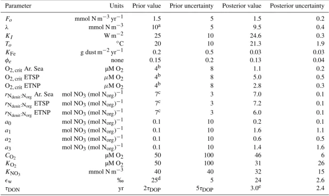
Table B1.Prior (pre-optimization) and posterior (post-optimization) values of the control parameters, and associated uncertainties. Prior uncertainties are 1 standard deviation of a normal distribution.
Parameter Units Prior value Prior uncertainty Posterior value Posterior uncertainty
Fo mmol N m−3yr−1 1.5 5 1.5 0.2
λ mmol N m−3 10a 5 9.5 0.4
KI W m−2 25 10 24.6 0.3
To ◦C 20 10 21.3 1.9
KFe g dust m−2yr−1 0.2 0.5 0.03 0.03
φe none 0.15 0.2 0.13 0.04
O2, critAr. Sea µM O2 4b 8 1.1 0.2
O2, critETSP µM O2 4b 8 5.0 0.5
O2, critETNP µM O2 4b 8 2.8 0.3
rNdenit:NorgAr. Sea mol NO3(mol Norg)
−1 7c 3 7.0 0.1
rNdenit:NorgETSP mol NO3(mol Norg)
−1 7c 3 7.2 0.1
rNdenit:NorgETNP mol NO3(mol Norg)
−1 7c 3 6.0 0.1
a0 mol NO3(mol Norg)−1 0.1 10 0.2 0.1
a1 mol NO3(mol Norg)−1 0.1 10 1.6 1.1
a2 mol NO3(mol Norg)−1 0.1 10 0.6 0.5
a3 mol NO3(mol Norg)−1 0.1 10 1.4 1.6
CO2 µM O2 50 100 46 6
KO2 µM O2 50 100 31 26
KNO3 mmol N m
−3 40 40 32 15
ǫw ‰ 25d 5 24 2.6
τDON yr 2τDOP 5τDOP 3.0e 2.4
aHoll and Montoya (2005),bCodispoti et al. (2005),cPaulmier et al. (2009),dBarford et al. (1999),eDepends on value ofσ
DONused and varies from
0.4±0.1 yr forσDON=2/3, to 6.6±0.8 yr forσDON=1/4.
the ratio of NO3 consumed to organic N remineralized, or
in the critical O2threshold for denitrification) to effectively
make up for any biases in the value ofbwithin suboxic zones. Several other variables were held fixed (i.e., not included as control parameters of the inverse model) including the isotopic enrichment factors for nitrogen fixation (ǫfix),
ben-thic denitrification (ǫb), and assimilation of nitrate to form
organic matter (ǫup), which are fixed at various values in
different model configurations; and the fraction of organic nitrogen routed to the DON pool (σDON), which is fixed at
eitherσDOPor 0.5σDOP, depending on the model
configura-tion. The values ofǫb,ǫfix,ǫup, andσDONused in the different
model configurations are given in Sect. 2.2.
In total, there are 21 parameters that are iteratively ad-justed to find the optimal solution (Table B1). The adjustable parameters include 6 parameters controlling the rate and spa-tial pattern of N2fixation (Fo,λ,To,KI,KFe,φe); 6 param-eters controlling the rate and spatial pattern of water-column denitrification (O2,,critandrNdenit:Norgare allowed to vary
sep-arately in the Indian Ocean, the South Pacific, and the North Pacific); 7 parameters controlling the rate and spatial pat-tern of benthic denitrification (a0−a3,CO2,KO2,KNO3); the
timescale for remineralization of DON (τDON); and the
en-richment factor for water-column denitrification (ǫwcd).
The optimal solution is defined as the set of control param-eters that minimize the following cost function:
c= 1
nN∗σ2
N∗
X
(N∗(mod)−N∗(obs))2
+ 1
nδσδ215NO 3
X
(δ15NO3(mod)−δ15NO3(obs))2 (B1)
+ 1
npσp2
X
(ppos−ppri)2,
wherenN∗(nδ) is the number of grid cells with N∗(δ15NO3)
observations, andnp=21 is the number of control parame-ters.pposrepresents the final (posterior) value of the model
parameters, andppritheir prior values, which were used as
the initial guess (see Table B1). We choseσp2to be very large for all parameters so that the model solution was not biased toward our initial guess. In all solutions, the value of the last term in Eq. (B1) is much smaller than the value of the first two terms.
each of which necessitates computing the steady-state solu-tion to the model equasolu-tions. This large number of simulasolu-tions is made possible by applying Newton’s method to the nonlin-ear nitrogen cycle equations, which allows rapid convergence to a steady-state solution.
Table B1 lists the control parameters of the inverse model, their initial guesses and their final values. The initial guesses for parameter values were set by published estimates where available, and by hand tuning to achieve rough consis-tency with observations for parameters without a published estimate. The final (post-optimization) parameter values are the mean of the values at the end of each of the 48 different optimizations (using different values ofǫfix,ǫb, andσDON),
and the uncertainty is the standard deviation of each parame-ter in this set of 48 optimal solutions. We should note that the quasi-Newton algorithm cannot distinguish between global and local minima. However, most parameters have a rela-tively small posterior uncertainty indicating a strong min-imum (Table B1). Some parameters have a large posterior uncertainty (e.g., KO2), which might reflect multiple local
minima in that parameter, but more likely reflects a broad, weak minimum indicating that these parameters are poorly constrained.
Acknowledgements. Constructive reviews by N. Gruber and an anonymous referee helped to improve the quality of the manuscript. Funding for this research was provided by NSF grant OCE-1131548 and the Gordon and Betty Moore Foundation. F. Primeau acknowledges support from NSF grant OCE-1131768.
Edited by: J. Middelburg
References
Alkhatib, M., Lehmann, M. F., and del Giorgio, P. A.: The ni-trogen isotope effect of benthic remineralization-nitrification-denitrification coupling in an estuarine environment, Biogeo-sciences, 9, 1633–1646, doi:10.5194/bg-9-1633-2012, 2012. Altabet, M. A.: Constraints on oceanic N balance/imbalance
from sedimentary 15N records, Biogeosciences, 4, 75–86, doi:10.5194/bg-4-75-2007, 2007.
Anderson, L. A. and Sarmiento, J. L.: Refield ratios of remineraliza-tion determined by nutrient data analysis, Global Biogeochem. Cy., 8, 65–80, 1994.
Barford, C. C., Montoya, J. P., Altabet, M. A., and Mitchell, R.: Steady-state nitrogen isotope effects of N2and N2Oproduction inParacoccus denitrificans, Appl. Environ. Microbiol., 65, 989– 994, 1999.
Bianchi, D., Dunne, J. P., Sarmiento, J. L., and Galbraith, E. D.: Data-based estimates of suboxia, denitrification, and N2O production in the ocean and their sensitivities to dissolved O2, Global Biogeochem. Cy., 26, GB2009, doi:10.1029/2011GB004209, 2012.
Bohlen, L., Dale, A. W., and Wallmann, K.: Simple transfer func-tions for calculating benthic fixed nitrogen losses and C:N : P
re-generation ratios in global biogeochemical models, Global Bio-geochem. Cy., 26, GB3029, doi:10.1029/2011GB004198, 2012. Botev, Z., Grotowski, J., and Kroese, D.: Kernel density estimation
via diffusion, Ann. Stat., 38, 2916–2957, 2010.
Brandes, J. A. and Devol, A. H.: Isotopic fractionation of oxygen and nitrogen in coastal marine sediments, Geochim. Cosmochim. Acta, 61, 1793–1801, 1997.
Brandes, J. A. and Devol, A. H.: A global marine-fixed nitrogen iso-topic budget: implications for Holocene nitrogen cycling, Global Biogeochem. Cy., 16, 1120, doi:10.1029/2001GB001856, 2002. Carpenter, E. J., Harvey, H. R., Fry, B., and Capone, D. G.: Biogeo-chemical tracers of the marine cyanobacteriumTrichodesmium, Deep Sea Res. Pt. I, 44, 27–38, 1997.
Codispoti, L. A.: An oceanic fixed nitrogen sink exceeding 400 Tg N yr−1 vs. the concept of homeostasis in the fixed-nitrogen inventory, Biogeosciences, 4, 233–253, doi:10.5194/bg-4-233-2007, 2007.
Codispoti, L. A., Brandes, J. A., Christensen, J. P., Devol, A. H., Naqvi, S. W. A., Paerl, H. W., and Yoshinari, T.: The oceanic fixed nitrogen and nitrous oxide budgets: moving targets as we enter the anthropocene, Sci. Mar., 65, 85–105, 2001.
Codispoti, L. A., Yoshinari, T., and Devol, A. H.: Suboxic respi-ration in the oceanic water column, in: Respirespi-ration in Aquatic Ecosystems, edited by: del Giorgio, P. A. and le B. Williams, P. J., Oxford Univ. Press, New York, 225–247, 2005.
De Pol Holz, R., Robinson, R. S., Hebbeln, D., Sigman, D. M., and Ulloa, O.: Controls on sedimentary nitrogen isotopes along the Chile margin, Deep-Sea Res. Pt. II, 56, 1100–1112, 2009. Deutsch, C., Sigman, D. M., Thunell, R. C., Meckler, A. N., and
Haug, G. H.: Isotopic constraints on glacial-interglacial changes in the oceanic nitrogen budget, Global Biogeochem. Cy., 18, GB4012, doi:10.1029/2003GB002189, 2004.
Deutsch, C., Sarmiento, J. L., Sigman, D. M., Gruber, N., and Dunne, J. P.: Spatial coupling of nitrogen inputs and losses in the global ocean, Nature, 445, 163–167, 2007.
Devol, A. H. and Christensen, J. P.: Benthic fluxes and nitrogen cy-cling in sediments of the continental margin of the Eastern North Pacific, J. Mar. Res., 51, 345–372, 1993.
Devol, A. H., Codispoti, L. A., and Christensen, J. P.: Summer and winter denitrification rates in Western arctic shelf sediments, Cont. Shelf Res., 17, 1029–1050, 1997.
DeVries, T. and Primeau, F.: Dynamically- and observationally-constrained estimates of water-mass distributions and ages in the global ocean, J. Phys. Oceanogr., 41, 2381–2401, 2011. DeVries, T., Deutsch, C., Primeau, F., Chang, B., and Devol, A.:
Global rates of water-column denitrification derived from nitro-gen gas measurements, Nat. Geosci., 5, 547–550, 2012. DiFiore, P. J., Sigman, D. M., and Dunbar, R. B.: Upper ocean
gen fluxes in the Polar Antarctic Zone: constraints from the nitro-gen and oxynitro-gen isotopes of nitrate, Geochem. Geophy. Geosy., 10, Q11016, doi:10.1029/2009GC002468, 2009.
Eugster, O. and Gruber, N.: A probabilistic estimate of global ma-rine N-fixation and denitrification, Global Biogeochem. Cy., 26, doi:10.1029/2012GB004300, 2012.