www.geosci-model-dev.net/8/1275/2015/ doi:10.5194/gmd-8-1275-2015
© Author(s) 2015. CC Attribution 3.0 License.
A stabilized finite element method for calculating balance velocities
in ice sheets
D. Brinkerhoff1and J. Johnson2
1Geophysical Institute, University of Alaska, Fairbanks, USA
2Group for Quantitative Study of Snow and Ice, University of Montana, Missoula, USA Correspondence to:D. Brinkerhoff ([email protected])
Received: 30 May 2014 – Published in Geosci. Model Dev. Discuss.: 8 August 2014 Revised: 21 February 2015 – Accepted: 11 March 2015 – Published: 4 May 2015
Abstract. We present a numerical method for calculating vertically averaged velocity fields using a mass conservation approach, commonly known as balance velocities. This al-lows for an unstructured grid, is not dependent on a heuristic flow routing algorithm, and is both parallelizable and effi-cient. We apply the method to calculate depth-averaged ve-locities of the Greenland Ice Sheet, and find that the method produces grid-independent velocity fields for a sufficient pa-rameterization of horizontal plane stresses on flow directions. We show that balance velocity can be used as the forward model for a constrained optimization problem that can be used to fill gaps and smooth strong gradients in InSAR ve-locity fields.
1 Introduction
Balance velocities are useful in evaluating the dynamics of ice sheets, as a means to fill missing velocity data (e.g., Joughin et al., 2010), and as an additional point of compar-ison for data-derived and modeled velocities (Bamber et al., 2000). Stemming from a statement of mass conservation, bal-ance velocity provides an intuitive means for understanding the distribution of flux within an ice sheet. It has often pro-vided estimates of velocity with better fidelity to data than even advanced ice sheet models, while relying on fewer as-sumptions. It also gives us the means to assess the distance from equilibrium of an extant ice sheet.
Heretofore, balance velocity has been calculated by ap-plying discrete routing algorithms to spatially distribute flux. These have traditionally been drawn from the hydrological literature (e.g., Tarboton, 1997; Budd and Warner, 1996). To
leading order, hydrological routing and glaciological routing are similar; flow directions in both cases are governed by driving stresses, which are determined by surface slope. In overland routing of liquid water, this method is appropriate. However, in glacial ice, the flow direction is also determined by horizontal plane stresses (and, to a lesser extent, vertical resistive stresses), and neglecting these terms yields an over-convergent pattern. This emphasis on local slopes also tends to exacerbate grid dependence, causing the same routing al-gorithm to produce markedly different velocity fields for dif-ferent grid resolutions (LeBrocq et al., 2006). Algorithms overcome this by using a spatially averaged slope rather than a purely local slope, with smoothing lengths and the shape of the averaging filter derived heuristically (Testut et al., 2003) or from theoretical results of parameterizing horizontal plane stresses (Kamb and Echelmeyer, 1986).
In addition to the novel, but basic, method for computing balance velocities, we also present a method by which bal-ance velocities can be used to fill gaps and smooth spurious gradients in InSAR-derived velocity data (e.g., Joughin et al., 2010). This is often advantageous, since further applications, such as inversion for basal traction or computing local stress balances, depend on having a smooth and complete velocity field. The method relies on minimizing a misfit functional over the velocity field with respect to error bounded thick-ness, apparent surface mass balance, and flow direction.
2 Continuum formulation
For an incompressible fluid, conservation of mass is stated as
∇ ·u=0, (1)
where u is the three-dimensional fluid velocity field, with kinematic boundary conditions on the surfaceSand bedB
∂S
∂t +uk(S)· ∇kS=w(S)+ ˙a (2) and
∂B
∂t +uk(B)· ∇kB=w(B)−mb, (3) respectively. Vertically integrating Eq. (1), applying the Leib-niz rule, and substitution of Eqs. (2) and (3) yields a ver-tically averaged statement for conservation of mass, com-monly called the continuity equation
∂H
∂t + ∇k·ukH= ˙a−mb, (4) with surface mass balance a, basal melt˙ mb, and thickness H.∇k·is the divergence operator in the two horizontal di-rections, anduk= [u, v]is the vertically averaged horizontal velocity vector. We henceforth drop the parallel bars, and as-sume that all vectors and operators work on the horizontal plane. This equation is well known to ice sheet modelers as the prognostic equation for evolving the geometry of an ice sheet. In this case, we assume an estimate of∂tH, and group
it with the other source terms, yielding
∇ ·uH=F, (5)
whereF = ˙a−mb−∂tH. Equation (5) is often used to
calcu-lateH (Morlighem et al., 2011; Johnson et al., 2012). Here, we assume thatH is known, and instead use Eq. (5) to cal-culateu. As stated, the system is underdetermined, with only one equation for both velocity components. For closure, we restate the problem in terms of flow directionN and speed U=kuk2(wherek ·k2denotes the standardL2norm), such that
NU=u,kNk2=1. (6)
This gives the scalar equation for unknownU
∇ ·NH U =F. (7)
Flow direction is specified as the solution to the problems
τs= ∇ ·(lH )2∇τs−τd (8)
with boundary condition
∇τs·n=0 on∂ (9)
and
N= τs kτsk2
. (10)
The solution to Eq. (8) is equivalent to the application of a Gaussian average of variable length scalelH to the driv-ing stressτdof the type suggested by Kamb and Echelmeyer (1986). Theoretical work typically expresses stress coupling length scales in terms of ice thicknesses, hence the nota-tionlH;l is the number of ice thicknesses over which hor-izontal plane stress coupling should act. Flow directionN
is then proportional to the smoothed driving stressτs with unit normalization. In the case where the boundary of the computational domain corresponds to the complete bound-ary of an ice mass (balance velocity for all of Greenland, say), no boundary condition need be specified, as the solu-tion is implicitly defined to be zero at the ice divide due to the problem geometry. When considering a partial domain, a Dirichlet condition must be specified once per flow line.
3 Discretization and stabilization
Equations (5), (8), and (10) are closed, and can be used to calculate balance velocity. We use the finite element method in order to discretize the governing equations. Equation (8) can be discretized with standard Galerkin methods (e.g., Zienkiewicz and Taylor, 2000). Its weak form is
Z
τs·φ+∇φ·(lH )2∇τsd= − Z
τd·φd,
∀φ∈H1×H1, (11)
here attempting to solve for velocity rather than thickness. This means that velocity and thickness switch roles in the stabilization scheme; U is advected by the pseudo-velocity
NH. The SUPG weak form is Z
(λ+τ∇ ·NH λ)(∇ ·NH U−F )d=0,
∀λ∈V , (12)
whereλ is a test function that accommodates the influx or outflux Dirichlet boundary condition if so specified, V = {λ∈H1, λ|Ŵ=0};τ is a mesh-dependent stabilization
pa-rameter given by τ = h
2kNHk2
, (13)
andhis the element circumradius. We use linear Lagrange finite elements for discretization. The inclusion of this un-usual stabilization term is key to achieving meaningful nu-merical solutions; without it, the solutions are plagued by non-physical oscillations. This instability is likely the reason that this approach has not been seen in the literature previ-ously.
4 Application to the Greenland Ice Sheet
We apply this balance velocity approach to the Greenland Ice Sheet. We used the 1 km gridded GLAS/ICESat data set (DiMarzio et al., 2007) for surface elevations and a bed DEM from Bamber et al. (2001) for bed elevations. Annual average surface mass balance rates are derived from RACMO (Et-tema et al., 2009). We assume that basal melt is small com-pared to surface mass balance, and neglect it. We also assume that the∂tH is negligible, or that the ice sheet is in balance.
This is doubtless an incorrect assumption in some regions of the ice sheet, but although estimates for this field exist (e.g., Pritchard et al., 2009), it is not yet possible to determine what proportion of this signal is a result of ice dynamics, as opposed to other mechanisms such as firn densification that should not be included here.
4.1 Grid dependence
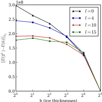
In order to assess the degree of grid dependence exhibited by this solution method, we start with a very coarse mesh, with an element circumradius of h=32H and calculate balance velocity over progressively finer meshes, essentially halving the element size at each iteration, down to an element cir-cumradius ofh=H or 500 m, whichever is greater. We do this for smoothing lengths l∈ {0,4,10,15}. The difference between the coarse solution and progressively finer solutions is shown in Fig. 1. We see that for smoothing lengths of l∈ {4,10,15}the norm of the difference between the refined and unrefined solutions stops changing with increasing re-finement. When l=0, the solution continues to change as
20 21 22 23 24 25 h (ice thicknesses)
0.0 0.5 1.0 1.5 2.0 2.5 3.0
||
¯ U(2 5 )− ¯ U(h)
||L2
1e8
l =0
l =4
l =10
l =15
Figure 1.Residual between balance velocity solution at coarse and progressively finer length scales forl∈ {0,4,10,15}.
the mesh becomes more refined. This indicates that incorpo-rating a parameterization of horizontal plane stress in flow routing can overcome the tendency for the flow field to over-converge, even for very finely resolved meshes.
4.2 Flow direction smoothing radius
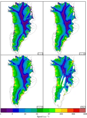
Figure 2.Balance velocity solution for a mesh size ofh=H and
l∈ {4,10,15}as well as InSAR surface velocities.
velocity fields. The northeastern ice stream, while apparent, is less significant than indicated by observations. Atl=15, features begin to wash out, most notably the characteristic multi-pronged ice streams of Kangerdlugssuaq glacier.
5 Application: physics-based interpolation of the surface velocity
Here, we present an application of our new technique for de-termining the balance velocity. The application is one that relies on many thousands of evaluations of the continuity equation in order to numerically optimize model output. It is conceptually and mathematically similar to the technique described by Morlighem et al. (2011), but with balance thick-nesses exchanged for balance velocities. For reasons of com-putational expense, our example could not be done without the advances presented earlier in this paper.
Geophysical data describing the cryosphere are in many cases incomplete or inconsistent with physical law. For ex-ample, take the surface velocity data of Joughin et al. (2010). They are characterized by large gaps in coverage and a highly variable structure in regions having low speed (less than
∼20 m a−1). Attributed to regions of high accumulation, high surface slopes, or incomplete satellite data, these prob-lem regions frustrate many efforts that depend on complete coverage, or smoothness of the data. Applications affected might include inversion for basal traction (Morlighem et al., 2013; Brinkerhoff and Johnson, 2013) or calculations involv-ing derivatives, such as resolvinvolv-ing the stress balance (Van der Veen, 2013).
In order to use such data, practitioners are often required to smooth and/or interpolate the data. The fundamental pro-cedure of interpolation is to generate a function that (1) is continuously valued over a given domain, (2) obeys some fundamental functional form between data points, and (3) adheres to observed values where data exist, with the under-standing that such data are subject to error. Standard inter-polation techniques often use polynomials as an interpolant. Physics-based interpolation differs by using solutions to the mass conservation partial differential equation (PDE) as the interpolating function. It is convenient to formulate this pro-cedure as an optimization problem, which minimizes some measure of misfit between data values under the constraint of mass conservation. In particular, we are interested in mini-mizing the misfit between (possibly incomplete) velocity ob-servations and balance velocities. This is expressed symboli-cally as
I′[U ,uo, H,N, F;λ]
=I[Um,uo] +F[N, U , H, F;λ] +R[N, H, F], (14) whereI is a misfit functional,F a functional that imposes continuity, and R a Tikhonov regularization used to im-pose a specified smoothness on the parameters. We depart from the previous notation by introducing balance velocity UmN, and observed velocity,uo, in order to keep the
quan-tities being compared clear. We define the observed speed Uo=kuok2. Finding the saddle point of Eq. (14) is known as PDE-constrained optimization.
5.1 Functional forms
I can take on a variety of forms. Here, we write a linear combination of least squares and log-least squares, or
I=
Z
e
α(Um−Uo)2+βln Uo Um
!2
d, (15)
whereeis the domain over which velocity observations
conservation of mass
F=
Z
λ ∇ ·NU H−Fd, (16)
whereλ is a Lagrange multiplier. Note that this PDE con-straint is still hyperbolic and requires the special numerical treatment defined previously in this paper.Ris a Tikhonov regularization term that penalizes large gradients in the values of explanatory parameters; f ∈P≡ {F, H,N}. We adopt the following form:
R=X
i
ξi Z
∇fi· ∇fid, (17)
foriin the space of explanatory parameters.ξi is a
regular-ization parameter. 5.2 Solution method
Consider the following, simplified, form of the PDE con-strained optimization problem:
I′=
Z
e
1
2 Um−Uo 2
dx+ Z
λ ∇ ·UNH−Fd. (18)
In practice we add a logarithm squared of the mismatch and regularization on each of the variables. However, this discussion neglects the terms to clarify the procedure that fol-lows. Because each of the fields appearing in the continuity equation is measured in some way, we express the uncertain-ties in the measurements as follows:
H ∈ [Ho−1Ho, Ho+1Ho] (19) F ∈ [F−1F, F+1F] (20)
N ∈ [N−1N,N+1N]. (21) Thus, we state that the admissible spaces for the explana-tory variables are defined by their assumed errors. Note that any choice within this range is assumed equally valid.
The mass conservation constraint, or forward model, is solved in two stages. First the directions of flow,N, are esti-mated from smoothed driving stress directions using the so-lution to Eq. (8). In regions where the direction of flow has been observed, N is replaced with the observed direction. The entire field is then smoothed to avoid large discontinu-ities on the boundaries between observed and estimated di-rections. The smoothing used takes the same form as Eq. ( 8). Equation (12) is used to express the stabilized form of the forward model. The original problem, Eq. (18), can now be restated in terms of the stabilized PDE constraint as
I′ =
Z
e
1
2 Um−Uo 2
d
+ Z
(λ+τ∇ ·NH λ)
| {z }
λ′
∇ ·NH Um−Fd, (22)
where the Lagrange multiplier plays the role of a test func-tion. To simplify the mathematics to follow, identify λ′=
λ+τ∇ ·NH λand recover the original form stated in Eq. (18), theλ′replacingλ.
We then take the first variation (formally a Gâteaux deriva-tive) ofI[U , H, F,N;λ′]with respect to each of its parame-ters. For instance, the variation with respect to the thickness His
δI′[Um, δH, F,N, λ] = ∂ ∂ǫ
ǫ=0
I′[Um, H+ǫδH, F,N, λ]. (23)
We note that a complete variation would have considered the error structure in observed speed,Uo, as well, but given the large areas of missing data, we did not include this in the analysis.
After varying the functional with respect to all terms, the result is
δI′ = Z
e
Um−Uo
δUm
| {z }
Adjoint RHS d
+ Z
λ′[∇ · δUmNH
| {z }
Adjoint LHS
+ ∇ · UmNδH
| {z }
gH
+ ∇ · UmH δN
| {z }
gN − δF |{z} gF ]d + Z
δλ′ ∇ ·UmNH−F
| {z }
Forward model d,
where we have ignored the dependence ofλon N andH. We also ignore variation with respect toU. Note that we can immediately identify individual terms specifying search di-rections (gi) for each of the variablesi∈ {H,NF}, as well
as the forward and adjoint models.
A few practical concerns arise, and are addressed as fol-lows.
1. δNis ambiguous, because it is a vector. However, only one component of a normalized vector is independent; i.e.,n2x+n2y=1 can be solved for an unknown. In this example, the variation is always done onδny.
2. Regularization is applied to each of the variables as shown in Eq. (17). L-curve analysis suggests that val-ues ofξi between 107 and 108 are reasonable. In this
example, all values were set to 107.
Figure 3. Surface speed of ice from observations reported in Joughin et al. (2010).
4. To make direct comparison of speeds, we need to es-timate vertically averaged velocities from surface ve-locity (Joughin et al., 2010). To do so, we construct a function that approximates the role of deformation in the observed surface velocity. The function makes ve-locities above 120 m a−1almost entirely due to sliding (surface velocity is the vertical average), and velocities below 25 m a−1nearly entirely due to deformation (sur-face velocity is 80% of the vertical average). A smooth transition between the two end members is given by the logistic function
Uo=f (Uo)
=Uo
1.0− .2
1+exp .1(Uo−75)
. (24)
5. The weighting between logarithmic and linear terms in the misfit functional of Eq. (15) is set to beα=β=0.5.
Figure 4.Final surface speeds, computed through the optimization of the speed constrained by the continuity equation described in this paper.
Under this weighting choice, in fast flowing regions, the linear misfit is dominant, while in slow flowing regions, the logarithmic misfit is more important.
5.3 Errors and numerical details
For the ice thickness field, data are drawn from Bamber et al. (2013). These data represent the reduction and interpolation of hundreds of individual radar tracks into a map having complete coverage. Bamber et al. (2013) report errors along tracks of zero. Here, we use±35 m along tracks, to reflect that there may be some error in the measurements. Off the tracks, we use the same values reported in Bamber et al. (2013).
Figure 5.Differences between the ice thicknesses reported in Bam-ber et al. (2013) and the thicknesses found at the end of the opti-mization procedure.
data are characterized by larger errors than other inputs, we shall assume very large errors in the apparent mass balance,
±1 m a−1.
The errors in the direction of the velocity reflect both dif-ferences from smoothed steepest descent where there are no velocity observations, as well as errors in the velocity obser-vations. We assumed these to be in the range±5◦.
All results were computed on an unstructured finite el-ement mesh with an average spacing between nodes of 2 km. The optimization was done by using the gradients, gH, gF, gN, to drive the quasi-Newton bounded
optimiza-tion technique, BFGSB (Nocedal and Wright, 2006). The
Figure 6.Apparent surface mass balance determined at the end of the optimization procedure.
optimization was terminated when the value of the objec-tive function ceased to change appreciably, less than 0.5 % through searches along each of the gradients.
5.4 Results and discussion
which accumulates ice flux along flow lines. The interpo-lation scheme also diffuses the channelized nature of flow in the lower Jakobshavn area, and perhaps in other outlet glaciers as well.
Our approach also provides thickness and effective mass balance (F) values that satisfy the continuity equation (Figs. 5 and 6). The changes made in order to uphold con-tinuity are quite significant but still within the assumed er-ror structure of the fields. In order to reproduce the observed speed in the outlet glaciers, thinner ice is required. This is due to the modeled velocity being too low; dividing the flux by a smaller thickness would increase the velocity. The bias toward slower ice could result from accumulation being too low, or velocity directions not being convergent enough. Ap-parent mass balance demonstrates that the search algorithm is utilizing this field to delimit streaming behavior by creat-ing gradient in mass balance across the margins.
Changes in the direction of flow,N, were less significant due to the low errors assumed in this field. There was little systematic change in values and it is difficult to interpret how the optimization process impacts the values.
Moreover, the results demonstrate that it is difficult to up-hold continuity and match the observed velocities. It is likely that the optimization is finding its way into a local minimum that is difficult to get out of. Once in this minimum, system-atic changes in the surface mass balance and thickness fields are made in a manner that is not likely to be physically plau-sible, but is reasonable in terms of the stated error bounds. The technique presented here should improve in its utility as the coverage of fundamental data sets increases, and un-certainties decrease. Eventually, the minimum reached from the initial point will better correspond to a global rather than local one. One application of this approach will be to pro-vide self-consistent initialization data for prognostic ice sheet modeling. Because the continuity is upheld by the data with a Lagrange multiplier, we are guaranteed that the combina-tion of thickness, mass balance, and velocity produced by this method will not produce the strong gradients in model output produced by data in which flux divergence does not equal apparent mass balance (Perego et al., 2014).
6 Conclusions
We presented a novel numerical method for calculating the balance velocity of an ice sheet using the finite element method. This approach is an advance over classical routing techniques because it is not dependent on a heuristic routing algorithm and relies solely on a continuum conservation law and a theoretically motivated parameterization of flow direc-tions. An unstructured grid easily allows for variable spatial resolutions. This method is made possible by two specific insights. First, flow directions that include horizontal plane stresses can be calculated by applying a spatially variable dif-fusion operator to the driving stress. Second, the balance
ve-locity equations can be viewed as an advection equation with a pseudo-velocity field specified by thickness and flow di-rection, with velocity as the advected quantity. This problem is unstable. We use the streamline upwind Petrov–Galerkin method to make it tractable.
We applied this method to the Greenland Ice Sheet. Bal-ance velocities were calculated over a number of different mesh resolutions, and we found that for given sufficient hor-izontal plane stress coupling distances, the solution shows grid independence. We also showed the balance velocity field calculated for theoretically justifiable smoothing lengths on detailed meshes. The resulting balance velocity compares fa-vorably with a satellite-measured velocity field.
Additionally, we presented a numerical method that uses adjoint-based optimization to both fill data gaps and smooth spurious gradients present in an InSAR-derived velocity data set. This method is conceptually similar to Morlighem et al. (2011), but minimizes the misfit between balance velocities and observation, as opposed to thickness. We showed that we can find a balance velocity that matches InSAR data well, but does not possess gaps or strong gradients, while re-maining within specified error bounds for input data fields. Despite this, we also find that upholding mass conserva-tion requires surface mass balance and thickness fields that are distinctly less smooth than those reported. Regardless, this PDE-constrained interpolation technique promises to be a useful tool for providing smooth and continuous velocity data that conform well to observations.
Acknowledgements. This work was made possible by NASA grant NASA EPSCoR NNX11AM12A. We thank the editor Philippe Huybrechts, as well as James Fastook and an anonymous reviewer, whose comments greatly increased the quality of the manuscript.
Edited by: P. Huybrechts
References
Bamber, J. L., Vaughan, D. G., and Joughin, I.: Widespread com-plex flow in the interior of the Antarctic Ice Sheet, Science, 287, 1248–1250, 2000.
Bamber, J. L., Layberry, R. L., and Gogineni, S. P.: A new ice thick-ness and bed data set for the Greenland Ice Sheet 1. measure-ment, data reduction, and errors, J. Geophys. Res., 106, 33773– 33780, 2001.
Bamber, J. L., Griggs, J. A., Hurkmans, R. T. W. L., Dowdeswell, J. A., Gogineni, S. P., Howat, I., Mouginot, J., Paden, J., Palmer, S., Rignot, E., and Steinhage, D.: A new bed elevation dataset for Greenland, The Cryosphere, 7, 499–510, doi:10.5194/tc-7-499-2013, 2013.
Var-GlaS, The Cryosphere, 7, 1161–1184, doi:10.5194/tc-7-1161-2013, 2013.
Brooks, A. N. and Hughes, T. J.: Streamline upwind/Petrov-Galerkin formulations for convection dominated flows with par-ticular emphasis on the incompressible Navier-Stokes equations, Comput. Method. Appl. M., 32, 199–259, doi:10.1016/0045-7825(82)90071-8, 1982.
Budd, W. F. and Warner, R. C.: A computer scheme for rapid cal-culations of balance-flux distributions, Ann. Glaciol., 23, 21–27, 1996.
DiMarzio, J., Brenner, A., Schutz, R., Shuman, C. A., and Zwally, H. J.: GLAS/ICESat 1 km laser altimetry digital elevation model of Greenland, Digital Media, Boulder, CO, USA: National Snow and Ice Data Center, 2007.
Ettema, J., van den Broeke, M. R., van Meijgaard, E., van de Berg, W. J., Bamber, J. L., Box, J. E., and Bales, R. C.: Higher sur-face mass balance of the Greenland Ice Sheet revealed by high-resolution climate modeling, Geophys. Res. Lett., 36, L12501, doi:10.1029/2009GL038110, 2009.
Fricker, H. A., Warner, R. C., and Allison, I.: Mass balance of the Lambert Glacier/Amery Ice Shelf system, East Antarctica: a comparison of computed balance fluxes and measured fluxes, J. Glaciol., 46, 561–570, doi:10.3189/172756500781832765, 2000.
Johnson, J. V., Brinkerhoff, D. J., Nowicki, S., Plummer, J., and Sack, K.: Estimation and propagation of errors in ice sheet bed elevation measurements, in Scientific Program, AGU Fall Meet-ing, 2012.
Joughin, I., Fahnestock, M., Ekholm, S., and Kwok, R.: Balance velocities of the Greenland Ice Sheet, Geophys. Res. Lett., 24, 3045–3048, doi:10.1029/97GL53151, 1997.
Joughin, I., Smith, B. E., Howat, I. M., Scambos, T., and Moon, T.: Greenland flow variability from ice-sheet-wide velocity mapping, J. Glaciol., 56, 415–430, doi:10.3189/002214310792447734, 2010.
Kamb, B. and Echelmeyer, K.: Stress-gradient coupling in glacier flow: I. longitudinal averaging of the influence of ice thickness and surface slope, J. Glaciol., 32, 267–284, 1986.
Larour, E., Seroussi, H., Morlighem, M., and Rignot, E.: Continen-tal scale, high order, high spatial resolution, ice sheet modeling using the Ice Sheet System Model (ISSM), J. Geophys. Res.-Earth, 117, F01022, doi:10.1029/2011JF002140, 2012.
LeBrocq, A. M. L., Payne, A. J., and Siegert, M. J.: West Antarctic balance calculations: Impact of flux-routing algorithm, smooth-ing algorithm and topography, Computers and Geosciences, 32, 1780–1795, doi:10.1016/j.cageo.2006.05.003, 2006.
Logg, A., Mardal, K.-A., and Wells, G. N. (Eds.): Automated So-lution of Differential Equations by the Finite Element Method, Springer, New York, doi:10.1007/978-3-642-23099-8, 2012. Morlighem, M., Rignot, E., Seroussi, H., Larour, E., Ben Dhia,
H., and Aubry, D.: A mass conservation approach for map-ping glacier ice thickness, Geophys. Res. Lett., 38, L19503, doi:10.1029/2011GL048659, 2011.
Morlighem, M., Seroussi, H., Larour, E., and Rignot, E.: Inver-sion of basal friction in Antarctica using exact and incomplete adjoints of a higher-order model, J. Geophys. Res.-Earth, 113, doi:10.1002/jgrf.20125, 1746–1753, 2013.
Nocedal, J. and Wright, S.: Numerical Optimization, 2nd ed., Springer, New York, 2006.
Perego, M., Price, S., and Stadler, G.: Optimal initial conditions for coupling ice sheet models to Earth system models, J. Geophys. Res.-Earth, 119, 1894–1917, doi:10.1002/2014JF003181, 2014. Pritchard, H. D., Arthern, R. J., Vaughan, D. G., and Edwards,
L. A.: Extensive dynamic thinning on the margins of the Greenland and Antarctic Ice Sheets, Nature, 461, 971–975, doi:10.1038/nature08471, 2009.
Seddik, H., Greve, R., Zwinger, T., Gillet-Chaulet, F., and Gagliar-dini, O.: Simulations of the Greenland Ice Sheet 100 years into the future with the Full Stokes model Elmer/Ice, J. Glaciol., 58, 427–440, 2012.
Tarboton, D. G.: A new method for the determination of flow di-rections and upslope areas in grid digital elevation models, Wa-ter Resources Research, 33, 309–319, doi:10.1029/96WR03137, 1997.
Testut, L., Hurd, R., Coleman, R., Rémy, F., and Legrésy, B.: Com-parison between computed balance velocities and GPS mea-surements in the Lambert Glacier Basin, East Antarctica, Ann. Glaciol., 37, 337–343, 2003.
Van der Veen, C. J: Fundamentals of Glacier Dynamics, 2nd ed., CRC Press, 2013.