www.hydrol-earth-syst-sci.net/15/2025/2011/ doi:10.5194/hess-15-2025-2011
© Author(s) 2011. CC Attribution 3.0 License.
Earth System
Sciences
A framework for the quantitative assessment of climate change
impacts on water-related activities at the basin scale
D. Anghileri, F. Pianosi, and R. Soncini-Sessa
Dipartimento di Elettronica e Informazione, Politecnico di Milano, Milano, Italy
Received: 17 December 2010 – Published in Hydrol. Earth Syst. Sci. Discuss.: 19 January 2011 Revised: 1 June 2011 – Accepted: 14 June 2011 – Published: 28 June 2011
Abstract. While quantitative assessment of the climate change impact on hydrology at the basin scale is quite ad-dressed in the literature, extension of quantitative analysis to impact on the ecological, economic and social sphere is still limited, although well recognized as a key issue to sup-port water resource planning and promote public participa-tion. In this paper we propose a framework for assessing climate change impact on water-related activities at the basin scale. The specific features of our approach are that: (i) the impact quantification is based on a set of performance indi-cators defined together with the stakeholders, thus explicitly taking into account the water-users preferences; (ii) the man-agement policies are obtained by optimal control techniques, linking stakeholder expectations and decision-making; (iii) the multi-objective nature of the management problem is fully preserved by simulating a set of Pareto-optimal man-agement policies, which allows for evaluating not only vari-ations in the indicator values but also tradeoffs among con-flicting objectives. The framework is demonstrated by appli-cation to a real world case study, Lake Como basin (Italy). We show that the most conflicting water-related activities within the basin (i.e. hydropower production and agriculture) are likely to be negatively impacted by climate change. We discuss the robustness of the estimated impacts to the climate natural variability and the approximations in modeling the physical system and the socio-economic system, and perform an uncertainty analysis of several sources of uncertainty. We demonstrate that the contribution of natural climate uncer-tainty is rather remarkable and that, among different mod-elling uncertainty sources, the one from climate modeling is very significant.
Correspondence to:D. Anghileri ([email protected])
1 Introduction
Climate change emerged as one of the major forces that will affect water availability in the future (Bates et al., 2008). In the last 20 years, a great research effort has been de-voted to increasing our knowledge about atmospheric and ocean circulation and estimating future climatic scenarios. Unfortunately, the complexity and computational burden of circulation model do not allow for simulation at the local spatial scale where the impacts on water-related activities must be estimated. To fill the gap between global and local scale, many methods were developed to downscale General Circulation Model (GCM) and Regional Circulation Model (RCM) projections.
information on strategies to adapt to these impacts” (EEA, 2009, p.18, Sect. 1.2).
Quantitative assessment of climate change impacts on water-related activities, both in the biological and human sphere, is very complex, for several reasons.
First, if the analysis must account for the true expectations and needs of the water users, defining quantitative indicators requires a long and complex process of knowledge elicita-tion from experts and stakeholders’ representatives (Soncini-Sessa et al., 2007). This is not always straightforward, espe-cially when not strictly economic issues are concerned.
Second, the system management must be modeled. Some authors (Schaefli et al., 2007) try to reproduce the histori-cal management by inferring it from historihistori-cal time series; others (Ajami et al., 2008) propose and test different man-agement strategies. The former approach is questionable be-cause the system management is likely to change following changed meteo-hydrological conditions; the latter does not guarantee that the best adaptation policy has been consid-ered, confounding the effect of climate change with that of using a sub-optimal policy.
Finally, uncertainty deeply affect the impacts quantifica-tion. The evolution of socio-economic drivers, e.g. popula-tion growth and economic and technological development, cannot be exactly predicted. For given driver scenario, the response of the climate and water system is estimated by simulation models that inevitably exhibit structural and pa-rameter errors. All these uncertainties are propagated and possibly amplified in the modeling chain from the global cli-mate to the impact assessment (Schaefli et al., 2007). Un-certainty analysis must therefore be an integral part of any impact study.
Since taking into account all the uncertainty sources simul-taneously requires a huge computational effort, impact stud-ies usually analyse only the most relevant sources at the tem-poral and spatial scale of interest. For instance, Arnell (2004) assesses the hydrological implications of climate change us-ing several consistent climate and socio-economic scenarios. Brekke et al. (2009) analyse projections from 17 different GCMs, while Lopez et al. (2009) use an ensemble of projec-tions of the same GCM under different parametrizaprojec-tions or
perturbed physics ensembles. D`equ`e et al. (2007) compare the projection of many different RCMs on the European do-main, while Bronstert et al. (2007) compare three different downscaling methods to estimate the long-term water avail-ability, drought conditions and floods. Ajami et al. (2008) analyse uncertainty rising from different hydrological model structures and parametrizations.
Less attention is usually devoted to assessing the uncer-tainty due to the inner variability of climate ormulti-decadal variability(Arnell, 2003), which limits the statistical signifi-cance of any impact quantification based on finite time series of climatic variables, either observed or obtained by model simulation. Even if relevant, this aspect is disregarded by
many authors, possibly bringing to misleading impact assess-ments.
The purpose of this paper is to present a framework for the quantitative assessment of the climate change impacts on water-related activities and the associated uncertainty anal-ysis. The approach is demonstrated by application to Lake Como basin, Italy, a complex water system in the South-ern Alpine region. Briefly, it is composed of an irrigation-fed agricultural district downstream of the lake, which is one of the largest irrigated area in Europe, and of a hy-dropower reservoir network located in the lake catchment, which provides nearly 25 % of the national hydropower pro-duction. Other interests in play are preventing floods on the lake shores and preserving ecosystems both in the lake and along the river.
The novelties of our approach are the following: (1) the quantification of the impacts is based on a set of performance indicators defined together with the stakeholders representa-tives, thus explicitly taking into account the water users pref-erences; (2) the multi-objective nature of the management problem is fully preserved by simulating a set of Pareto-optimal management policies under different climatic sce-narios, which allows for evaluating not only variations in the indicator values but also tradeoffs among conflicting objec-tives; (3) uncertainty analysis results in deriving confidence bounds around the simulated Pareto frontiers.
Hydropower reservoir
Power plant
Como city Penstock River Adda
Ri ver Adda
Legend
Lake Como
Lake Como catchment
River
Irrigated area
0 4 8 16 24 32 40
Kilometers
Fig. 1.Lake Como water system.
2 Lake Como case study
Lake Como is a regulated lake in Northern Italy (Fig. 1). Its operative storage is about 254 Mm3and it is fed by a catch-ment of about 4550 km2. The catchment is characterized by the typical Alpine hydrological regime with low discharge in winter and summer and high in late spring and autumn. The current regulation of the lake aims at attenuating flood-ing along the lake shores, especially in Como city, and to sup-ply downstream users (5 irrigation districts and 9 run-of-river power plants) through a wide network of canals. The lake catchment area is covered by a dense network of smaller ar-tificial lakes operated for hydropower production. However the overall storage of hydropower reservoirs is of 510 M m3, more than twice the storage of the lake (OLL, 2005).
by increased water demand from the downstream irrigated areas due to the temperature raise.
In our analysis we will focus on two sectors: hydropower production in the upstream reservoirs and irrigation in the downstream areas. Presently, they are the main conflicting interest in the region: hydropower producers traditionally schedule their production in winter time and thus they store water in spring and summer when, on the contrary, the irri-gation demand is at top. The conflict is worsened in case of water scarcity, as happened in the summer droughts of 2003 and 2005, two of the most severe droughts in Europe in the last decade, so that climate change is expected to aggravate the situation. Protection from flooding in Como city will not be considered since a defence system consisting of mobile gates is currently under construction and thus the lake man-agement will soon become irrelevant to this purpose. Hy-dropower production in run-of-river plants downstream from the lake will also be neglected because its contribution is very limited.
From the modeling point of view, the Alpine hydropower reservoirs are described by one equivalent reservoir whose capacity is the sum of the total capacity of the actual reser-voirs. The simplification is acceptable because the reservoir storages are strongly correlated with each other. The differ-ent water users downstream of the lake are lumped into one equivalent downstream user, whose benefit/cost is related to the total water amount that is diverted from the lake efflu-ent (river Adda) to the main irrigation canals. The model-ing time step is one day, that is the decision time step cur-rently adopted by the lake manager. For more details on the model of the water system (catchments, reservoirs and river network) see Anghileri et al. (2011).
3 Assessment of the climate change impacts
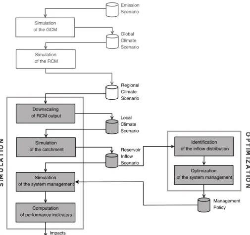
Traditional approaches to climate change impact assessment at the basin scale rely on a modeling chain that usually in-cludes the generation of future emission scenarios, the sim-ulation of GCM to build global climate scenarios, the use of RCM and statistical downscaling to estimate climate ios at the basin scale, and the projection of climatic scenar-ios into discharge scenarscenar-ios via simulation of hydrological models. The modeling chain often stops here, while further evaluation of hydrological scenarios is committed to experts. In this paper we extend quantitative assessment also to impacts on water-related activities like agriculture and hy-dropower generation. To this end, the modeling chain must be extended to include simulation of the water system man-agement and evaluation of the impacts by means of perfor-mance indicators (Fig. 2). Both tasks are not trivial since they require a deep knowledge of the system functioning in all its aspects, from engineering to social and economic issues.
The definition of performance indicators is a challeng-ing task, especially when not strictly economic issues are
concerned, e.g. impact of changed hydrological regime on the riparian ecosystems, or when the relation between water availability and economic outcome is complicated. For in-stance in the irrigation district downstream from Lake Como a reduction in the water supply from the canals can be par-tially compensated by pumping from groundwater, which saves the crop but is costly. Definition and validation of the indicators used in this study was performed by interacting with stakeholder representatives and deriving a set of crite-ria that reflects their judgments and expectations (Castelletti et al., 2007).
Simulating the system management is an issue because it requires modeling the behaviour of the managers of the reser-voirs and distribution network. In this study, we formulate the decision-making problem faced by the human regulators as an optimal control problem, and use multi-objective op-timization techniques to derive Pareto-optimal management policies (see right side of Fig. 2), thus obtaining an upper bound of system performances that may be achieved by a fully rational decision-maker (Soncini-Sessa et al., 2007). To link stakeholder expectations and decision-making pro-cess, we use the performance indicators defined by the stake-holder representatives as the objectives of the optimal control problem. Since the problem is a multi-objective one, the so-lution is not a unique optimal management policy but a set of Pareto-optimal policies, each providing a different trade-off between the conflicting objectives. Choosing one policy within this set is not a technical task but a political one, re-quiring subjective weighting of the objectives, and as such it must be left to stakeholders and decision-makers. There-fore our analysis will be conducted by considering the entire collection of Pareto-optimal policies.
In the next paragraph we will describe the modeling units developed for assessing the impact of climate change in the case study area of Lake Como basin. For the reader conve-nience, we define some of the terms that will be used in the following:
– historical climate: the time series of precipitation and temperature observed in the catchment (gauge records from 1967 to 1980)
– historical inflow: the time series of observed discharge from the catchment, flowing into the reservoirs (gauge records from 1967 to 1984)
– historical inflow scenario: the time series of simulated discharge obtained by feeding the catchment model with historical climate
Downscaling of RCM output
Simulation of the catchment
Simulation of the system management
Computation of performance indicators
Impacts
Optimization of the system management
Identification of the inflow distribution Local
Climate Scenario Regional Climate Scenario Global Climate Scenario Simulation
of the GCM
Simulation of the RCM
Reservoir Inflow Scenario Emission Scenario
Management Policy
Fig. 2. The procedure for quantitative assessment of climate change impacts on water-related activities: simulation tools on the left side, optimization tools on the right side.
– backcast (forecast) inflow scenario: the time series of simulated discharge obtained by feeding the catchment model with the backcast (forecast) climate scenario. 3.1 Downscaling procedure
The climate of the Alps is strongly influenced by local phe-nomena (orographic forcing, rain-shadowing, etc.). In such cases, RCMs provide more realistic climatic forecast at the regional scale with respect to GCMs, since the mismatch of scale between the resolution of the climate models and the scale of interest for regional impacts is lower (Mearns et al., 2003; Fowler et al., 2007; Frei et al., 2006). The cli-matic time series considered in this study were derived as part of a larger multimodel ensemble in the framework of the European project PRUDENCE (see http://prudence.dmi.dk/ and Christensen and Christensen, 2007). As backcast and forecast climate scenarios we considered the daily precipi-tation and mean temperature time series over the backcast period 1961–1990 and the forecast one 2071–2100 respec-tively. Each scenario was simulated using the emission sce-nario A2 (IPCC, 2000) and the GCM HadAM3H (Pope et al., 2000) as driving data.
Even if RCMs provide good estimate of the climate at the regional scale, some biases from the local climate of interest may still exist. In this study, RCMs’ output were corrected via the statistical downscaling method known as Quantile Mapping. For a given variable, the cumulative density func-tion (cdf) of the backcast is first matched with the cdf of the observations, thus generating a correction function depend-ing on the quantile. The correction function is then used to unbias the variable from the forecast quantile by quan-tile. This method has been used in many hydrological impact studies, using a correction function at either annual or sea-sonal level (D`equ`e, 2007; Bo`e et al., 2007).
J F M A M J J A S O N D
ï10 0 10 20 30
(°C)
a
J F M A M J J A S O N D 0
50 100 150 200
(mm)
b
J F M A M J J A S O N D 0
200 400 600 800 1000 1200
(mm)
c
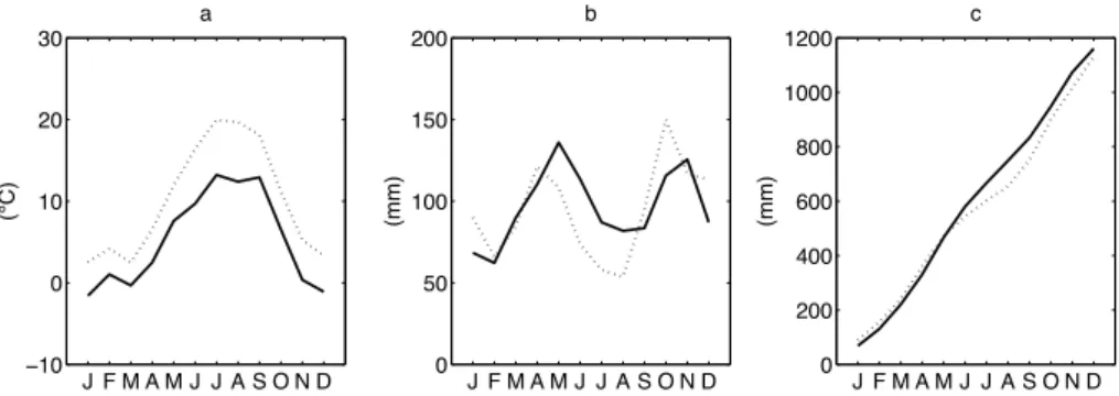
Fig. 3. Mean monthly temperature in the backcast (solid) and forecast (dotted) scenario(a); total monthly precipitation(b); and cumulate precipitation over the year(c)with downscaled RACMO RCM.
Figure 3 compares some statistics of the downscaled out-put of the RACMO RCM (Lenderink et al., 2003) over the backcast and forecast period. The forecast climate scenario shows an increase in monthly mean temperature (of about 4◦
C) and a shift in the precipitation pattern (decrease in spring and summer and increase in autumn and winter) while the annual precipitation volume is only slightly lower than in the backcast scenario.
3.2 Catchment model
The catchment response to climatic input is simulated through a lumped, conceptual model, partially based on the
HBV model (Bergstrom, 1976). The lumped modeling ap-proach guarantees efficient parameterization even with lim-ited historical time series. However spatial processes are ne-glected. In our case study spatial heterogeneity is not sig-nificant, but for elevation. Nonetheless comparison of our proposed model and an elevation-based model (Consorzio dell’Adda, 1986) shows that lumping does not induce sig-nificant loss of information.
Our model is composed of three modeling units. First, the precipitation input is splitted into snowfall and rainfall: aver-age daily temperature in a reference station is used to deter-mine the freezing level and snowfall is computed as a fraction of the total precipitation, through a proportionality coeffi-cient that accounts for the catchment’s area located above the freezing level. Then, the snowpack dynamics is described by a mass balance equation, while a degree-day approach is used to determine the snowmelt. Finally, theHBVmodel is used to simulate the soil water balance and subsequent runoff, as a consequence of melt-water, rainfall, and evapotranspiration. The latter is computed throught the Blaney-Criddle method (Brouwer and Heibloem, 1986).
Two different parametrizations were used for the two catchment, the one feeding the equivalent hydropower reser-voir (catchment surface area of about 350 km2) and the other feeding Lake Como (4200 km2). They were derived using the Genetic Algorithm implemented in the Matlab Global Optimization Toolbox and time series of daily precipitation,
Table 1. Parameterers of the optimally calibratedHBVmodel for the lake Como (LC) catchment and the hydropower reservoir (HR) catchment, and relevant performance indicators over the validation dataset (1977–1984).
model parameters LC HR FC maximum soil moisture content (mm) 251.9 238.5 LP limit for potential evapotranspiration 1 0.9 ALFA response box parameter 0.04 0.02 BETA exponential parameter in soil routine 0.14 1.06 K recession coefficient for upper tank 0.29 0.11
(day−1)
K4 recession coefficient for lower tank 0.04 0.04 (day−1)
PERC maximum flow from upper to lower 6.98 0 tank (mm day−1)
CFLUX maximum value of capillarity flow 0 0 (mm day−1)
MAXBAS transfer function parameter (day) 1.01 1.21 performance indicators
R2 coefficient of determination (−) 0.654 0.799 MAE mean absolute error (m3s−1) 57.5 3.22
RVE relative volume error (−) 0.23 0.09
temperature and flow. Precipitation is the spatial average from several meteorological stations; temperature data come from two reference stations, one for each of the two catch-ments; flow data are derived by inversion of the reservoir mass balance equations. The objective function of the auto-matic calibration procedure is the coefficient of determina-tion (one minus the ratio between error variance and mea-sured flow variance). Table 1 shows the optimal parameter values of theHBV soil-moisture routine for the two catch-ments.
Fig. 4. Left: observed vs simulated flow from lake Como catchment (top) and hydropower reservoir catchment (bottom) in the validation period (1977–1980). Right: observed flow (dots) and simulated flow (grey line) in 1980.
and simulated flow (Fig. 4). They show that the model er-ror is quite significant especially for high flow. Nonetheless the model accuracy is acceptable for the scope of this study, as we will show in Sect. 4.1.
Note that in this study we did not include a model of the glacier dynamics. At present, the contribution of glacier melting is usually negligible but for extremely hot and dry summer periods, as for instance the 2003 drought. How-ever, under future climate scenario of increased temperature, glacier melting may become relevant. Also, there exist mul-tiple evidences of a constant glacier reduction since from the beginning of the 20th century (Smiraglia and Diolaiuti, 2006), which means that glacier melting may give a positive contribution to flow in the middle-term while disappearing in the long run. However, such an evolution cannot be repro-duced in our study.
3.3 Reservoir and management model
The water system reservoir network is modeled by two reser-voir in cascade: the equivalent hydropower reserreser-voir and Lake Como. Each reservoir is described by the mass balance equation
sit+1 = sti +qti+1 −Ri sti, uit, qti+1 (1)
wheresti is the storage at timet of thei-th reservoir,qti+1
is the inflow from its catchment, uit is the release decision
taken at timetandRi (sti, uit, qti+1)is the release that actu-ally occured in the interval [t,t+ 1), which may differ from
uit because of unintentional spill or other physical or legal constraints (Soncini-Sessa et al., 2007).
paper, we will use the set of management policies reported therein as the reference to evaluate how things may change under climate change. It consists of eight different policies, each corresponding to a different tradeoff of the two objec-tives, including the two extreme policies that consider either irrigation or hydropower only.
3.4 Performance indicators
The definition of indicators was developed together with the stakeholder representatives in a former research project (Castelletti et al., 2007). In that project, a representative per-son for each stakeholder group was identified. These are: the managers of the hydropower companies; the leaders of the irrigation consortia (representative for the farmers); officials from Como city and other towns along the lake shores (rep-resentative for the flooding, navigation, fishing and tourism issues); the manager of the Nature Park located along the lake effluent river. The indicators were identified by struc-tured interviews and validated during a final meeting, where each stakeholder representative was asked to rank different situations and it was checked that the ranking was consistent with the one determined by the indicator.
In this study we focus only on the hydropower and irriga-tion indicators: a brief descripirriga-tion of the two follows, while a detailed definition is given in Anghileri et al. (2011).
The hydropower indicator is the average daily revenue from hydropower production
Jhyd = 1
h
h−1
X
t=0
nt+1
X
j=0
θt,j G (2)
wherehis the length of the simulation horizon, used to evalu-ate the system performances;nt+1is the number of working
hours of the plant on dayt (equal to the release rt1+1 from the equivalent hydropower reservoir divided by the power plant capacity); G is the energy produced per hour, when the plant is working at full capacity; andθt,j is the energy price in thej-th most profitable hour of dayt. The energy price is a periodic parameter. Its weekly and annual pattern is estimated from time series of energy price over the period 2005–2006 provided by the national energy authority (see www.mercatoelettrico.org).
The irrigation indicator is the squared daily deficit in the water supply
Jirr = 1
h
h−1
X
t=0
h
maxWt −rt2+1,0
i2
(3)
wherert2+1is the release from Lake Como in the time interval [t,t+ 1) andWt is the water demand for irrigation on dayt. The water demand is a periodic parameter. Its annual pattern is estimated combining the water requirement declared in the abstraction licenses and the historical time series of diverted flows. Power 2 in Eq. (3) is a means to implicitely select
management policies that reduce high-percentage deficit in a single time step while allowing for more frequent small shortages, which cause less damage to the crop.
3.5 Impact assessment
The performance indicators were used when designing the optimal management policies. In fact, the objective functions of the stochastic optimal control problem are the expected values of Eqs. (2) and (3) with respect to all the possible trajectories of the inflows (i.e. the inflow probability distri-bution) over an infinite horizon (h → ∞). Note that, since
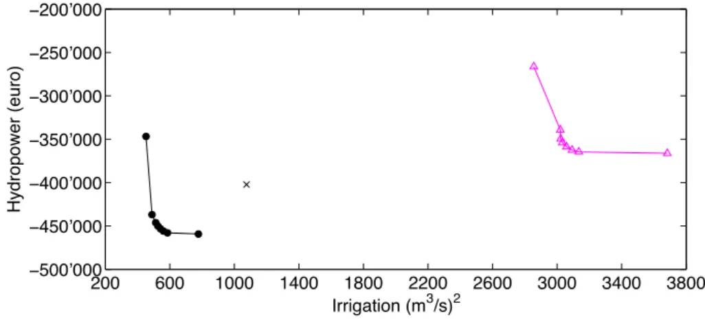
the inflow probability distribution is estimated over histor-ical time series, the result is optimal as long as the hydro-logical behaviour of the system remains stationary. For each Pareto-optimal policy reported in Anghileri et al. (2011), the expected values of the indicators can be assessed by Markov or Monte Carlo simulation. Alternatively, it is possible to use deterministic simulation and compute the indicator val-ues over a single finite horizon. The latter approach is com-putationally less demanding and can provide a more infor-mative output to stakeholders: for instance, using a histori-cal horizon they can compare the simulated behaviour of the system with the historical one, which they directly experi-mented. The performance indicators under the historical in-flow over the period 1967–1984 are shown in Fig. 5 (black dots). Note that even if produced by Pareto-optimal poli-cies, they do not necessarily belong to the Pareto Frontier of the two-objective control problem, as they are obtained under historical inflow and not under the inflow probability distribution used in optimization. For this reason they will be called the Image of the Pareto Frontier (IPF). It can be no-ticed that the historical IPF (black dots in Fig. 5) can greatly improve the satisfaction of both the water users with respect to the historical management (cross in Fig. 5) and represent an effective tool to mitigate the conflict between upstream and downstream water users.
200 600 1000 1400 1800 2200 2600 3000 3400 3800
ï500’000
ï450’000
ï400’000
ï350’000
ï300’000
ï250’000
ï200’000
Irrigation (m3/s)2
Hydropower (euro)
Fig. 5. Image of the Pareto Frontier (IPF) under historical inflow 1967–1980 (black dots) and forecast inflow scenario 2071–2100 by RACMO RCM (magenta triangles). The cross is the historical management. Hydropower revenue (on the vertical axis) is changed in sign.
200 400 600 800 1000 1200 1400 ï480’000
ï460’000 ï440’000 ï420’000 ï400’000 ï380’000 ï360’000 ï340’000 ï320’000
Irrigation (m3/s)2
Hydropower (euro)
(a)
200 400 600 800 1000 1200 1400 ï480’000
ï460’000 ï440’000 ï420’000 ï400’000 ï380’000 ï360’000 ï340’000 ï320’000
(b)
Irrigation (m3/s)2
Fig. 6. Left panel: IPFs under historical inflow over a sliding window of 10 years between 1967 and 1984. Black dots are the IPF under historical inflow over the entire horizon 1967–1980. Rigth panel: IPFs under backcast inflow scenario over a sliding window of 14 years between 1961 and 1990. Black dots are the IPF under historical inflow scenario over the entire horizon 1967–1980.
3.6 Validation of the assessment procedure
The trustability of the results presented in the previous sec-tion depends on the robustness of the adopted simulasec-tion procedure, which is affected by two major sources of un-certainty. First, the comparison is based on indicator values computed over finite system trajectories. Would results be significantly different under a different choice of the simula-tion horizon? Second, as in any impact assessment analysis we shall consider what is the contribution of modeling errors. The latter problem will be discussed in the next section, here we will focus on the problem of using finite simulation hori-zon, which is an intrinsic issue of the assessment procedure independently of the modeling error issue.
To assess the uncertainty in the indicator values due to the choice of the simulation horizon, we computed seven
different IPFs with a sliding window of h= 10 years over the period 1967–1984 (grey dots in Fig. 6a). It can be seen that differences are generally small, exception made for two IPFs, which present a strongly lower irrigation cost: they cor-respond to simulation horizon that do not include the year 1973, characterized by one of the most severe droughts of the 20th century. The estimated indicator values are indeed sensitive to single extreme events occurring or not occurring in the selected horizon. The length of the horizon also af-fects the results. The historical IPF (black dots), although including the dry year 1973, shows lower irrigation costs be-cause the same events are averaged over a longer simulation horizon (14 years instead of 10).
200 600 1000 1400 1800 2200 2600 3000 3400 3800
ï500’000
ï450’000
ï400’000
ï350’000
ï300’000
ï250’000
ï200’000
Irrigation (m3/s)2
Hydropower (euro)
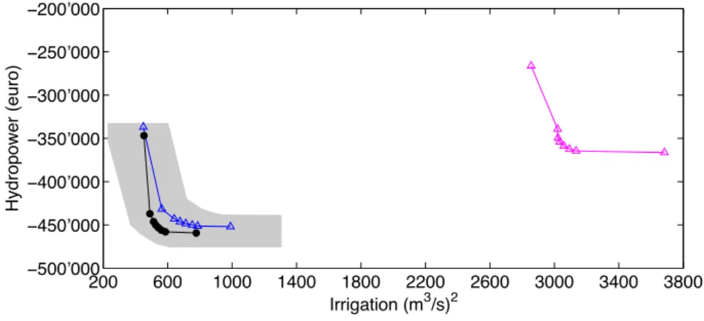
Fig. 7. IPF under historical inflow 1967–1980 (black dots), backcast inflow scenario 1961–1990 by RACMO RCM (blue triangles) and forecast inflow scenario 2071–2100 by RACMO RCM (magenta triangles). The grey region represents the natural variability of backcast climate scenario obtained as the envelope of the IPFs over a sliding window of 14 years reported in Fig. 6b.
precipitation and temperature, then projected into flows, can only be interpreted as equiprobable to observations (Royer, 2000). It follows that, even assuming that the RCM perfectly reproduced the climate dynamics (i.e. even neglecting the modeling error issue), we could not expect its output time series to perfectly overlap historical observations. Indeed, the observed climate over 1967–1980 is simply equiproba-ble to any 14-years long time series in the backcast period. To assess the uncertainty in the indicator values due to such statistical equiprobability, we computed several IPFs under the backcast scenario with a sliding window ofh= 14 years. They are shown in Fig. 6b: as expected, none of these IPFs is superimposed to the historical one, but they are scattered around it. Finally, the IPF under the entire backcast scenario of 30 years from 1961 to 1990 can be computed: it is rep-resented by the triangles in Fig. 7. This IPF may be used as a fair reference for comparison with the IPF under forecast scenario, in place of the historical IPF (1967–1984), since it is based on the same simulation model and horizon lengthh
as the forecast IPF.
Although the use of a finite horizon and the statistical in-terpretation of the RCM output do not allow for a univocal quantification of the system performances over the past, this intrinsic variability is negligible with respect to the variation that is expected to be induced by climate change, as shown in Fig. 7. This is consistent with other research: for instance, Arnell (2003) demonstrates that changes in mean seasonal discharge in many basins in Britain are outside the range of natural climate variability by 2050s, but that climate change signal and natural variability could be difficult to distinguish when considering nearer horizons.
4 Uncertainty analysis
In the previous paragraph, we showed how the natural vari-ability of the climate and the impossibility to use infinite time series (of observation or climate simulation) affect the robustness of the estimated impacts. Beside this intrinsic uncertainty in impact assessment, another source of uncer-tainty lays in the tools used to implement it, that is, the chain of simulation models shown in Fig. 2. We will distinguish two types of uncertainties: those introduced in modeling the physical system and those introduced in modeling the socio-economic system.
4.1 Uncertainty in modeling the physical system
The description of the physical system includes modeling the climate dynamics through the GCM, RCM and statistical downscaling; modeling the catchment response; and model-ing the reservoirs.
200 600 1000 1400 1800 2200 2600 3000 3400 3800 4200 4600 5000 5400
ï500’000
ï450’000
ï400’000
ï350’000
ï300’000
ï250’000
ï200’000
Irrigation (m3/s)2
Hydropower (euro)
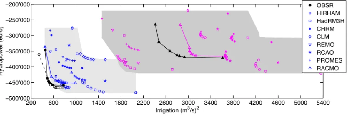
OBSR HIRHAM HadRM3H CHRM CLM REMO RCAO PROMES RACMO
Fig. 8.IPF under historical inflow 1967–1980 (black dots), IPF under historical inflow scenario 1967–1980 (white dots), IPFs under backcast inflow scenarios (1961–1990) using eight different RCM models (blue symbols), IPFs under forecast inflow scenarios (2071–2100) with the same eight different RCMs (magenta symbols), IPF under forecast RACMO inflow scenarios (2071–2100) using optimal management policies for future climate (black triangles).
can be considered as exact at the spatial and temporal scale of interest.
Besides structural uncertainty, the simulation output is also affected by parameter uncertainty. In particular for downscaling and the catchment model, the problem is that parametrizations were selected by minimization of the sim-ulation error over historical time series. This approach is highly questionable when the model is used for projecting future climate scenarios that are, by definition, violating the stationary assumption underlying calibration over historical time series. Unfortunately there is no solution to this para-dox: the past is the only testing ground we have to assess the validity of our models.
Regardless of the distinction between structural and pa-rameter uncertainty, the impact of the model error can be assessed, at least for the catchment model, by a simple ex-periment: to simulate the system under the historical inflow scenario, i.e. the discharge time series produced by the catch-ment model when fed by the historical climate. The corre-sponding IPF is shown in Fig. 8 (white dots). It can be seen that it does not perfectly overlap the historical IPF (black dots), as expected if there were no error in the catchment model. However the modeling error is rather limited com-pared to variability induced by the use of equiprobable cli-mate scenarios and the full range of indicator values is repro-duced.
As for the climate model, the impact of structural uncer-tainty may be assessed by simulating and comparing dif-ferent circulation models. Generally, since the winter cli-mate is mainly driven by global circulation while the sum-mer climate is largely influenced by local phenomena, the choice of the GCM is the main source of uncertainty in win-ter time, while the RCM is more important in the summer (Jacob et al., 2007). Besides this distinction, some studies (D`equ`e et al., 2007; Schaefli et al., 2007) seem to indicate that the choice of the GCM is the most critical. However, as for the RCM scenarios generated in the PRUDENCE project
and used in this analysis, Hingray et al. (2007) show that vari-ability among RCMs is comparable to the varivari-ability induced by the GCM choice. Following these considerations and for brevity’s sake, in this paper we will focus only on the RCM variability. Starting from the climate scenario from seven dif-ferent RCMs (beyond the RACMO model) provided by the PRUDENCE project, we applied the downscaling method to each of them and then projected climate input into inflow scenarios. Figure 8 shows the IPFs under these eight back-cast (blue) and foreback-cast (magenta) inflow scenarios. It can be seen that the spread of the IPFs is rather high even over the backcast scenario: the RACMO RCM, that we used so far as the reference model, produces an IPF quite close to the historical one, together with the REMO and HIRHAM, while other RCMs seem to be less accurate in reproducing the historical system performances. The spread of the IPFs strongly increases in the forecast scenario – although all fu-ture scenarios are derived from the same emission scenario, A2, and GCM boundary condition, HadAM3H.
To conclude, our study provides one more confirmation that circulation models, and specifically RCMs, are a ma-jor source of uncertainty in impact assessment studies, much more relevant than other sources like uncertainty from us-ing finite simulation horizon or inner climate variability, as it can be seen by comparing the extent of the uncertainty re-gions (grey area) in Figs. 6.a, b and 8. Notwithstanding this high uncertainty, comparison of the uncertainty regions over backcast and forecast scenarios (Fig. 8) suggests that a signif-icant worsening of the system performances can be expected: there is basically no overlapping between the backcast and forecast uncertainty region.
4.2 Uncertainty in modeling the socio-economic system
indicators. Uncertainty associated to these choices is rather different from uncertainty in modeling the physical system. In the latter case, uncertainty stems from our limited capacity of reproducing reality through models and, to some extent, it can be objectively quantified by comparison of model output with observations from the real system. Uncertainty in mod-eling the socio-economic system, instead, can rarely rely on observations or reference values. For instance, there is no exact choice of the emission scenario, and the only way to assess the impact of such choice is to repeat the entire simu-lation procedure under a different scenario.
The same holds for the choice of the performance indica-tors. Since they are aimed at reflecting the stakeholder pref-erences, stating whether they actually capture the stakeholder opinions is very difficult. For the hydropower producers, the choice of the revenue is rather straightforward, while for the farmers the definition of the indicator is more difficult. The proper choice would be the revenue from the crop produc-tion, however this indicator would need a model of the crop growth that is expensive to develop and often does not guar-antee reliable results. The average squared deficit that we used in our analysis is a proxy indicator easy to compute and that received the approval of the farmers’ representatives, and as such it is hardly questionable.
What can be argued is the value of the parameters inside the indicator formulation. So far, we implicitly assumed a business-as-usual scenario for the energy price and water de-mand. However, the pattern of energy price may change in the future following changed conditions in the energy mar-ket, while the water demand may be reduced thanks to im-provement in the irrigation technique (e.g. from submersion to more efficient systems) or changes in the crop. Climate change itself will probably drive such changes. Therefore, the analysis so far must not be interpreted as a prediction of the future conditions, which would be unrealistic because the socio-economic system will certainly evolve and adapt to re-duced water availability, but rather as the demonstration that the current socio-economic conditions cannot be maintained in the future.
The business-as-usual assumption involves also the sys-tem management. In fact, variations in the hydrological con-ditions, as well as potential variations in the energy price or water demand, will lead the reservoir managers to change their behaviour. In our analysis we simulated the manage-ment policies that proved Pareto-optimal over historical in-flow statistics, energy price, etc. but they will not be Pareto-optimal any more if these conditions will change. Even if we set aside the issue of energy prices or water demand, still the results shown so far are overly pessimistic because based on sub-optimal policies, and there is room for improvement by re-optimizing the management policies under the new in-flow scenarios. To explore this room for improvement, we ran the following experiment. We used the first years of the forecast inflow scenarios produced by the downscaled output of the RACMO RCM to re-estimate the probability
distribution of the reservoir inflows and, based on this new distribution, re-run Stochastic Dynamic Programming, thus obtaining eight Pareto-optimal policies for the new climate scenario. Then, we simulated the new policies under the en-tire forecasting horizon and derived the IPF represented by the black triangles in Fig. 8. It can be seen that the sys-tem performances improve with respect to the original, sub-optimal IPF (magenta triangles), especially for the irrigation objective. Nonetheless, the improvement is not sufficient to compensate for deteriorated hydro-climatic conditions, as it can be seen by comparison with the IPF under backcast in-flow scenario (blue triangles). Notice that the comparison between these two IPFs is not affected by uncertainty in mod-eling the manager behaviour, since in both cases we assume the best possible behaviour, in Pareto-sense, that a rational decision-maker could follow for the corresponding inflow scenario and the selected performance indicators.
5 Conclusions
This paper presents a general framework for the quantita-tive assessment of the climate change impacts on the water-related activities at the basin scale. The proposed simulation procedure starts from the downscaling of regional circulation model output, and through the projection into the hydrologi-cal input and simulation of the system management, ends up with the computation of performance indicators. One major feature of our approach is the multi-objective perspective that is preserved throughout the entire simulation procedure. In fact, instead of simply reproducing the current system man-agement, we first derive a set of Pareto-optimal policies and then simulate all of them over both the historical, backcast and forecast scenario. The advantage is that tradeoffs be-tween different objectives can be explored under present and future climate conditions, and further that the comparison of past and future performances is not affected by subjective choice of the management policy.
characterizing the measure under study, for instance a differ-ent yearly pattern of the water demand in the definition of the irrigation performance indicator.
The results are highly affected by uncertainty. We ana-lyzed both the uncertainty stemming from the inner variabil-ity of climate and the modeling uncertainty. The analysis proved that, although the contribution of the former is quite significant, it is negligible with respect to the latter. Also, among different sources of modeling uncertainty, the uncer-tainty in the climate modeling, specifically RCMs, seems to be the most significant. A reduction of this uncertainty may be expected when considering climate scenarios in the shorter term. As a result of these multiple uncertainties, the exact quantification of the impacts in terms of performance indicators is, at the state-of-the-art, not fully reliable. How-ever the comparison of the uncertainty regions where cur-rent and future performances are expected to fall, clearly indicates that a significant loss will be induced by climate change, especially for the irrigation sector.
In the case study area, most of the stakeholders were al-ready organized into associations with long-established pro-cedures for selecting their delegates and resolving disputes. This was a clear advantage in developing our study. How-ever, when stakeholders are fragmented and/or the analysis also includes issues where perceptions of individual stake-holders may be strongly different (like landscape changes or ecology), more sophisticated tools and spatial analysis should be considered to enhance true participation.
Several topics remain open for future research. For Lake Como system, the evaluation of climate change impacts should be extended to other important sectors like for in-stance ecosystem conservation. The system model should be improved, particularly the hydrological model of the catch-ment that, in its current version, does not include the glacier dynamics, and the uncertainty analysis may be further de-tailed considering the other sources of uncertainty (e.g. pa-rameter uncertainty) mentioned in this paper but not fully analyzed yet.
While increasing complexity and accuracy of the simula-tion model will increase the trustability of the results, we question this will be sufficient to compensate for the large uncertainty that affects the assessment analysis, because of the inner variability of climate, our limited capacity in re-producing the complex circulation dynamics, and the errors induced by mismatches in scale. Therefore we think that the research effort to improve the model accuracy should be coupled with an equal effort towards developing effective methods to evaluate model uncertainty and its propagation through impacts assessment studies. This is especially true when dealing with multi-objective problems, where mod-elling and optimization is aimed at providing the knowledge base for political discussion and decision-making, not at re-placing it. The role of uncertainty analysis in this process is very delicate. From the modeler standpoint, uncertainty analysis enhances the robustness of the assessment results,
while for political decision-makers it may be perceived as undermining their trustability. Communicating the informa-tion contained in the IPF graphs shown in this paper is dif-ficult and time consuming: it requires the decision-makers to make an effort towards understanding at least the general principles of the underlying assessment methodology; and the willingness to assimilate a sophisticated message rather than simple answers. Effective communication of modelling results and their associated uncertainty should become inte-gral part of the research in this area.
Acknowledgements. The authors are grateful to the anonymous
reviewers for their comments that helped to improve the paper. The research presented in this paper was partially sopported by
Fondazione Lombardia per l’Ambiente(www.flanet.org).
Edited by: D. Solomatine
References
Abbaspour, K. C., Faramarzi, M., Ghasemi, S. S., and Yang, H.: As-sessing the impact of climate change on water resources in Iran, Water Resour. Res., 45, W10434, doi:10.1029/2008WR007615, 2009.
Ajami, N. K., Hornberger, G. M., and Sunding, D. L.: Sustain-able water resource management under hydrological uncertainty, Water Resour. Res., 44, W11406, doi:10.1029/2007WR006736, 2008.
Anghileri, D., Soncini-Sessa, R., and Weber, E.: Joint management of irrigation and hydropower production in lake Como system, Tech. Rep. 2011.7, Dipartimento di Elettronica e Informazione, Politecnico di Milano, 2011.
Arnell, N. W.: Relative effects of multi-decadal climatic variability and changes in the mean and variability of climate due to global warming: future streamflows in Britain, J. Hydrol., 270, 195– 213, 2003.
Arnell, N. W.: Climate change and global water resources: SRES emissions and socio-economic scenarios, Global Environ. Change, 14, 31–52, 2004.
Bates, B., Kundzewicz, Z., Wu, S., and Palutikof, J.: Climate Change and Water, Tech. rep., IPCC, 2008.
Bergstrom, S.: Development and application of a conceptual runoff model for Scandinavian catchments, Tech. Rep. RH07, SMHI, Norrkoumlping, Sweden, 1976.
Bo`e, J., Terray, L., Habets, F., and Martin, E.: Statistical and dynamical downscaling of the Seine basin climate for hydro-meteorological studies, Int. J. Climatol., 27, 1643–1655, 2007. Brekke, L., Townsley, E., Harrison, A., Pruitt, T., Maurer, E. P.,
An-derson, J., and Dettinger, M. D.: Assessing reservoir operations risk under climate change, Water Resour. Res., 45, W04411, doi:10.1029/2008WR006941, 2009.
Bronstert, A., Kolokotronis, V., Schwandt, D., and Straub, H.: Comparison and evaluation of regional climate scenarios for hy-drological impact analysis: General scheme and application ex-ample, Int. J. Climatol., 27, 1579–1594, 2007.
Castelletti, A., Pianosi, F., Sachero, V., and Soncini-Sessa, R.: Re-ducing the Vulnerability of Societies to Water Related Risks at the Basin Scale, chap. TwoLe/P: a MODSS Implementing PIP Procedure for Participative Water Basin Planning, IAHS Press, Wallingford, UK, 2007.
Christensen, J. H. and Christensen, O. B.: A summary of the PRU-DENCE model projections of changes in European climate by the end of this century, Climatic Change, 81, 7–30, 2007. Christensen, N. S. and Lettenmaier, D. P.: A multimodel
ensem-ble approach to assessment of climate change impacts on the hydrology and water resources of the Colorado River Basin, Hy-drol. Earth Syst. Sci., 11, 1417–1434, doi:10.5194/hess-11-1417-2007, 2007.
Consorzio dell’Adda: Gli Afflussi al Lago di Como, Analisi statis-tiche e modelli di previsione e simulazione (The lake Como in-flows: Statistical Analisys and forecasting and simulation mod-els, in Italian), Tech. rep., Milano, 1986.
D`equ`e, M.: Frequency of precipitation and temperature extremes over France in an anthropogenic scenario: Model results and sta-tistical correction according to observed values, Global Planet. Change, 57, 16–26, 2007.
D`equ`e, M., Rowell, D. P., Luthi, D., Giorgi, F., Christensen, J. H., Rockel, B., Jacob, D., Kjellstrom, E., De Castro, M., and van den Hurk, B.: An intercomparison of regional climate simulations for Europe: assessing uncertainties in model projections, Climatic Change, 81, 53–70, 2007.
EEA: Regional climate change and adaptation – The Alps facing the challenge of changing water resources, Tech. Rep. 8, EEA, 2009.
Fowler, H. J., Blenkinsop, S., and Tebaldi, C.: Linking climate change modelling to impacts studies: recent advances in down-scaling techniques for hydrological modelling, Int. J. Climatol., 27, 1547–1578, 2007.
Frei, C., Scholl, R., Fukutome, S., Schmidli, J., and Vidale, P. L.: Future change of precipitation extremes in europe: an intercom-parison of scenarios from regional climate models, J. Geophys. Res., 111, D06105, doi:10.1029/2005JD005965, 2006.
Groves, D. G., Yates, D., and Tebaldi, C.: Developing and ap-plying uncertain global climate change projections for regional water management planning, Water Resour. Res., 44, W12413, doi:10.1029/2008WR006964, 2008.
Guariso, G., Rinaldi, S., and Soncini-Sessa, R.: The management of Lake Como: multiobjective analysis, Water Resour. Res., 22, 109–120, 1986.
Hingray, B., Mouhous, N., Mezghani, A., Bogner, K., Schaefli, B., and Musy, A.: Accounting for global-mean warming and scaling uncertainties in climate change impact studies: application to a regulated lake system, Hydrol. Earth Syst. Sci., 11, 1207–1226, doi:10.5194/hess-11-1207-2007, 2007.
IPCC: Special Report on Emission Scenarios, Tech. rep., IPCC, 2000.
Jacob, D., B¨arring, L., Christensen, O. B., Christensen, J. H., de Castro, M., D´equ´e, M., Giorgi, F., Hagemann, S., Hirschi, M., Jones, R., Kjellstr¨om, E., Lenderink, G., Rockel, B., S´anchez, E., Sch¨ar, C., Seneviratne, S. I., Somot, S., van Ulden, A., and van den Hurk, B.: An inter-comparison of regional climate mod-els for Europe: model performance in present-day climate, Cli-matic Change, 81, 31–52, 2007.
Jasper, K., Calanca, P., Gyalistras, D., and Fuhrer, J.: Differential impacts of climate change on the hydrology of two alpine river basins, Clim. Res., 26, 113–129, 2004.
Lenderink, G., van den Hurk, B., van Meijgaard, E., van Ulden, A., and Cuijpers, H.: Simulations of present day climate in RACMO2: first results and model developments, Tech. rep., Royal Netherlands Meteorological Institute, 2003.
Lopez, A., Fung, F., New, M., Watts, G., Weston, A., and Wilby, R. L.: From climate model ensembles to climate change impacts and adaptation: A case study of water resource management in the southwest of England, Water Resour. Res., 45, W08419, doi:10.1029/2008WR007499, 2009.
Mearns, L. O., Giorgi, F., Whetton, P., Pabon, D., Hulme, M., and Lal, M.: Guidelines for Use of Climate Scenarios Developed from Regional Climate Model Experiments, Tech. rep., IPCC, 2003.
OLL: Tech. rep., Regione Lombardia, ARPA Lombardia, Fon-dazione Lombardia per l’Ambiente e IRSA/CNR, 2005. Pope, V. D., Gallani, M. L., Rowntree, P. R., and Stratton, R. A.:
The impact of new physical parametrizations in the Hadley Cen-tre climate model: HadAM3, Clim. Dynam., 16, 123–146, 2000. Royer, J. F.: Numerical modeling of the global atmosphere in the climate system, chap. The GCM as a dynamical system, NATO Science Series C 550, Kluwer Academic Publishers, 29–58, 2000.
Schaefli, B., Hingray, B., and Musy, A.: Climate change and hydropower production in the Swiss Alps: quantification of potential impacts and related modelling uncertainties, Hydrol. Earth Syst. Sci., 11, 1191–1205, doi:10.5194/hess-11-1191-2007, 2007.
Smiraglia, C. and Diolaiuti, G.: L’acqua, una Risorsa per il Sis-tema Agricolo Lombardo, chap. I ghiacciai lombardi. Variazioni di una risorsa idrica, Water Resources Publications, ERSAF, Mi-lano, IT, 54–62, 2006.
Soncini-Sessa, R., Castelletti, A., and Weber, E.: Integrated and par-ticipatory water resources management, Theory, Elsevier, Ams-terdam, NL, 2007.