ACPD
10, 8189–8246, 2010Vertical structure of Antarctic tropospheric ozone
depletion events
A. E. Jones et al.
Title Page
Abstract Introduction
Conclusions References
Tables Figures
◭ ◮
◭ ◮
Back Close
Full Screen / Esc
Printer-friendly Version
Interactive Discussion Atmos. Chem. Phys. Discuss., 10, 8189–8246, 2010
www.atmos-chem-phys-discuss.net/10/8189/2010/ © Author(s) 2010. This work is distributed under the Creative Commons Attribution 3.0 License.
Atmospheric Chemistry and Physics Discussions
This discussion paper is/has been under review for the journal Atmospheric Chemistry and Physics (ACP). Please refer to the corresponding final paper in ACP if available.
Vertical structure of Antarctic
tropospheric ozone depletion events:
characteristics and broader implications
A. E. Jones1, P. S. Anderson1, E. W. Wolff1, H. K. Roscoe1, G. J. Marshall1, A. Richter2, N. Brough1, and S. R. Colwell1
1
British Antarctic Survey, Natural Environment Research Council, High Cross, Madingley Road, Cambridge, CB3 0ET, UK
2
Institute of Environmental Physics, University of Bremen, Otto-Hahn-Allee 1, 28359 Bremen, Germany
Received: 2 March 2010 – Accepted: 17 March 2010 – Published: 29 March 2010
Correspondence to: A. E. Jones ([email protected])
ACPD
10, 8189–8246, 2010Vertical structure of Antarctic tropospheric ozone
depletion events
A. E. Jones et al.
Title Page
Abstract Introduction
Conclusions References
Tables Figures
◭ ◮
◭ ◮
Back Close
Full Screen / Esc
Printer-friendly Version
Interactive Discussion
Abstract
The majority of tropospheric ozone depletion event (ODE) studies have focussed on time-series measurements, with comparatively few studies of the vertical component. Those that exist have almost exclusively used free-flying balloon-borne ozonesondes and almost all have been conducted in the Arctic. Here we use measurements from 5
two separate Antarctic field experiments to examine the vertical profile of ozone during Antarctic ODEs. We use tethersonde data to probe details in the lowest few hundred meters and find considerable structure in the profiles associated with complex atmo-spheric layering. The profiles were all measured at wind speeds less than 7 ms−1, and on each occasion the lowest inversion height lay between 10 m and 40 m. We also 10
use data from a free-flying ozonesonde study to select events where ozone depletion was recorded at altitudes >1 km above ground level. Using ERA-40 meteorological charts, we find that on every occasion the high altitude depletion was preceded by an atmospheric low pressure system. An examination of limited published ozonesonde data from other Antarctic stations shows this to be a consistent feature. Given the 15
link between BrO and ODEs, we also examine ground-based and satellite BrO mea-surements, and find a strong association between enhanced BrO and atmospheric low pressure systems. The results suggest that, in Antarctica, such depressions are re-sponsible for driving high altitude ODEs and for generating the large-scale BrO clouds observed from satellites. In the Arctic, the prevailing meteorology differs from that in 20
ACPD
10, 8189–8246, 2010Vertical structure of Antarctic tropospheric ozone
depletion events
A. E. Jones et al.
Title Page
Abstract Introduction
Conclusions References
Tables Figures
◭ ◮
◭ ◮
Back Close
Full Screen / Esc
Printer-friendly Version
Interactive Discussion
1 Introduction
The remarkable behaviour exhibited by tropospheric ozone during spring in both polar regions is well documented (see Simpson et al., 2007 for full overview). Concentrations of ozone can fall from background levels to below instrumentation detection limits and remain suppressed for timescales of the order of hours to days. These excursions are 5
observed sporadically from coastal locations, and are widely referred to as tropospheric ozone depletion events (ODEs). The ozone depletion is driven by halogen chemistry, most notably bromine, which has a source associated with the sea ice zone. The exact source(s) and mechanisms responsible for bromine-release are still subject to debate, but the combination of concentrated sea salt in a condensed phase substrate appears 10
to be a pre-requisite. Under these conditions, and with sufficient acidity, gaseous HOBr can react with sea salt bromide within the condensed phase and generate Br2 that is
then released to the atmosphere. Subsequent photolysis of this Br2generates Br rad-icals that can react with and destroy O3. Altogether, this process is referred to as the
“Bromine Explosion” (Fan and Jacob, 1992; Tang and McConnell, 1996; Vogt et al., 15
1996; Lehrer et al., 2004). Environmental, as well as chemical conditions are also crit-ical for ODEs. Various studies have suggested a role for temperature in driving ODEs (Tarasick and Bottenheim, 2002; Jacobi et al., 2006) although this influence remains debated (Bottenheim et al., 2009). The role played by meteorology has also been highlighted, with a critical influence both on the onset of ODEs and on their termination 20
(e.g. Hopper and Hart, 1994; Jones et al., 2006, 2009).
Surface ozone has been measured at a relatively large number of coastal research stations in both the Arctic and Antarctica (Helmig et al., 2007), and these data have been used in the majority of ODE studies. Recently, measurements over the frozen Arctic Ocean have been carried out from ships (Jacobi et al., 2006; Bottenheim et al., 25
ACPD
10, 8189–8246, 2010Vertical structure of Antarctic tropospheric ozone
depletion events
A. E. Jones et al.
Title Page
Abstract Introduction
Conclusions References
Tables Figures
◭ ◮
◭ ◮
Back Close
Full Screen / Esc
Printer-friendly Version
Interactive Discussion However, ODEs are 4-dimensional phenomena, with structure in the horizontal and
vertical components as well as in time. Relatively few measurements have been made of the vertical profile of ozone, given the demands of such a procedure. Those that ex-ist, however, have revealed important information. For example, it appears that ozone depletion generally extends from the surface up to a few 100 s of meters, but that oc-5
casionally depletion to a few kilometres is observed (Solberg et al. 1996; Bottenheim et al., 2002; Strong et al., 2002; Tarasick and Bottenheim, 2002; Ridley et al., 2003; Wessel et al., 1998). Sometimes ozone depleted air can be observed at several kilo-metres altitude while ozone at the surface is normal (Wessel et al., 1998; Roscoe et al., 2001). Further, the vertical extent of an ODE appears to be strongly modulated 10
by the physical behaviour of the atmosphere, with temperature inversions forming the upper boundary of depleted air masses (e.g. Wessel et al., 1998; Strong et al., 2002; Tarasick and Bottenheim, 2002).
The studies referenced above were all carried out using ozonesondes on free-flying balloons. These balloons and their payload access the ozone profile throughout the 15
whole of the troposphere providing information on, for example, the height to which ODEs extend. They are highly effective at providing the broad vertical picture. How-ever, the balloons rise rapidly so that, with the time required to make an ozone mea-surement, the vertical resolution is limited to∼100 m. As a result, much of the detail
in the profile is not accessible. An alternative to a free-flying system is offered by teth-20
ered platforms, such as blimps. They are limited in height by the additional weight of the tether line, but tethered platforms enable slow controlled vertical ascent and descent rates. They thus enable significantly enhanced measurement resolution with vastly increased detail in the ozone profile information. Only one tethersonde study of springtime tropospheric ozone has been reported in which one Arctic ODE was probed 25
in detail (Anlauf et al., 1994). The data, presented at a resolution of ∼17 m, show a
ACPD
10, 8189–8246, 2010Vertical structure of Antarctic tropospheric ozone
depletion events
A. E. Jones et al.
Title Page
Abstract Introduction
Conclusions References
Tables Figures
◭ ◮
◭ ◮
Back Close
Full Screen / Esc
Printer-friendly Version
Interactive Discussion There is thus considerable merit in both profiling techniques, with each revealing
different, but complimentary, information.
In terms of data coverage, the overriding majority of ozone profiling studies published to date have been carried out in the Arctic. Thus far, only one study using ozonesondes to focuss on the Antarctic troposphere has been published (Wessel et al., 1998), and a 5
few profiles measured from on-going launch programmes at Neumayer and McMurdo stations have been used as supporting data (Kreher et al., 1997; Roscoe et al., 2001; Frieß et al., 2004).
In this paper we analyse data from two separate field experiments and use the results to explore the characteristics and implications of low- and high-altitude tropospheric 10
ozone depletion events. The first, a tethersonde experiment carried out in spring 2007, allows us to probe details in the lowest few hundred meters of the ozone profile and to explore the influence of the complex layering within this region of the atmosphere. The second was a programme of free-flying ozonesondes that was carried out at Halley during austral spring 1987. The experiment was aimed at measuring profiles of strato-15
spheric ozone, and the observations made in the troposphere have not previously been analysed. The data enable us to select cases of high altitude ozone depletion (i.e. ex-tending of the order 1 to∼3 km above ground level) as a starting point for teasing out
mechanisms driving ODE chemistry on wider spatial scales. The combined results en-able us to move towards a generalised picture of ODEs in Antarctica and assess their 20
implications and the challenges for modelling them both on local and regional scales.
2 Location
The measurements reported here were made at the British Antarctic Survey station, Halley, in the Weddell Sea sector of coastal Antarctica (Fig. 1). The tethersonde ex-periment of 2007 was carried out at Halley V station (75◦35′S, 26◦34′W) while the 25
ACPD
10, 8189–8246, 2010Vertical structure of Antarctic tropospheric ozone
depletion events
A. E. Jones et al.
Title Page
Abstract Introduction
Conclusions References
Tables Figures
◭ ◮
◭ ◮
Back Close
Full Screen / Esc
Printer-friendly Version
Interactive Discussion Halley sits on the floating Brunt Ice shelf, 32 m a.s.l. The surrounding area is
snow-covered, but flat and featureless, with the nearest rock outcrops roughly 200 km away. Halley is roughly 15 km inland from the permanent ice edge, and as the coast effectively forms a promontory at this point, the station is close to the Weddell Sea in three direc-tions. During springtime, the Weddell Sea is extensively covered in ice, interspersed 5
with open water leads, of note being a large polynya to the south west of Halley known as Precious Bay (Anderson, 2003). To the east of Halley is the inland ice, and indeed, the prevailing wind direction at Halley is easterly. Beyond the grounding line to the south east of Halley, continental ice rises to the polar plateau. Katabatic winds from the plateau descend towards Halley, but remain aloft of the station, above a cold pool 10
below (Renfrew et al., 2002). For a significant amount of the time during spring, air arrives at the base from across the sea ice zone. There is thus a range of air masses with different histories in the vicinity of Halley.
3 Methodology
3.1 The 2007 tethersonde study
15
A variety of instruments and techniques were used during the 2007 experiment with measurements for surface ozone, ground-based routine meteorology, sondes for mea-suring profiles of ozone and temperature, and an acoustic radar that highlights lay-ers of atmospheric turbulence and thus provides considerable context for the profile data. Ideally, profiles of ozone would be measured on a continuous basis, in order 20
to provide maximum information. However, as tethersonde experiments are highly labour-intensive, it was necessary instead to make targeted measurements. This was achieved using the surface ozone monitor: when a rapid decline in surface ozone mix-ing ratios was measured, an alarm triggered which alerted the overwintermix-ing staff to the onset of an event and the chance to initiate a profiling experiment. It is worth noting 25
ACPD
10, 8189–8246, 2010Vertical structure of Antarctic tropospheric ozone
depletion events
A. E. Jones et al.
Title Page
Abstract Introduction
Conclusions References
Tables Figures
◭ ◮
◭ ◮
Back Close
Full Screen / Esc
Printer-friendly Version
Interactive Discussion so that all the ODEs probed using this method occurred at Halley at wind speeds less
than 7 ms−1.
3.1.1 Surface ozone and routine meteorology
Measurements of wind speed and direction are carried out on a routine basis at Halley. The anemometers and wind vanes are located near to the main station, at a height 5
roughly 10 m above the snow surface. The data have an accuracy of about 0.5 ms−1 for wind speed and 5◦ for wind direction (K ¨onig-Langlo et al., 1998) and are available at 1-min resolution.
Surface ozone was measured at the Halley Clean Air Sector Laboratory (CASLab), which is located roughly 1 km from the station generators, and in a sector that re-10
ceives minimal contamination from the base (Jones et al., 2008). Surface ozone was measured year-round during 2007 using a Thermo Electron Corp. model 49C. The instrument uses a UV absorbance technique and has a detection limit of 1 ppbv (parts per billion by volume) and a precision of 1 ppbv for 1-min averages of 10-s data.
3.1.2 Blimp profiling system
15
In order to provide detail in the very lowest region of the atmosphere, we employed a tethered AB400 blimp (Cameron Balloons Ltd) as the airborne platform, which allowed a controlled and indeed variable ascent/descent rate. The blimp was able to carry a payload of ∼2 kg (in addition to the tether line) and was made of lightweight fabric
(LAM30) that had been used successfully in previous profiling experiments carried out 20
at low temperatures (Rankin and Wolff, 2002). The blimp had an internal volume of 11.3 m3, and was stored inflated inside a 4S Weatherhaven between experiments. A single reel (1000 m length) of 2 mm diameter Dyneema SK75 performance cord (Dy-namic) (English Braids Ltd) was used as the tether line, providing a balance between tensile strength (900 kg breaking load) and weight. The ascent/descent rate for the 25
ACPD
10, 8189–8246, 2010Vertical structure of Antarctic tropospheric ozone
depletion events
A. E. Jones et al.
Title Page
Abstract Introduction
Conclusions References
Tables Figures
◭ ◮
◭ ◮
Back Close
Full Screen / Esc
Printer-friendly Version
Interactive Discussion time constant of the ECC sonde (see below), yielded a vertical measurement resolution
of between 4 and 19 m (varying from flight to flight) with a mean of 11 m.
3.1.3 Vertical profiles of ozone and temperature
Ozone was monitored using an electro-chemical cell (ECC) sonde (Komhyr, 1969, 1995). The sondes were Science Pump Corp. Model 5A, with customised electronics, 5
powered by three 9 V lithium cells in parallel. No correction was required for reduction in pump speed with height given that these were tropospheric measurements. However, below a battery voltage of 2.9 V, the pump voltage would fluctuate, resulting in fluctu-ating pump speeds. Data were therefore rejected once the battery voltage dropped below 2.9 V. The other calibration factors vary by a few percent depending on the con-10
centration of KI and buffers, but the calibration is otherwise close to absolute (standard formula given by Komhyr et al., 1995). For tropospheric measurements, where the partial pressure of ozone is small, errors in calibration are generally small compared to errors in determining the zero of the measurement (see below).
Before a flight, a sonde was prepared and the output signal checked using an 15
ozoniser set to deliver about 50 ppbv. The zero was checked by sampling through an active charcoal filter – if zero did not stabilise to within a few tens of mV of the zero of the electronics (250 mV) within 10 minutes, the sonde was set aside and another prepared. The zero was again checked outside before a flight.
The ozonesonde signal was transmitted to the ground via external inputs to a 20
custom-made meteorological sonde. The meteorological sonde included a wind vane, a radio transmitter (Radiometrix, 10 mW at 173 MHz), a temperature compensated pressure sensor (Vaisala PTB100B, resolution 0.1 hPa), a temperature sensor (Be-tatherm 1K7A329I, accuracy 0.2 K), and 3 rotating wind cups on a near-vertical axis with rotating disc and optical counter sampling speed for 1 s intervals. It also in-25
ACPD
10, 8189–8246, 2010Vertical structure of Antarctic tropospheric ozone
depletion events
A. E. Jones et al.
Title Page
Abstract Introduction
Conclusions References
Tables Figures
◭ ◮
◭ ◮
Back Close
Full Screen / Esc
Printer-friendly Version
Interactive Discussion microcontroller (Parallax STAMP II) and a 14-bit digitiser with 8 channel multiplexer
(AD7856). Sensors were sampled once every 10 s before powering the transmitter for a few ms to transmit data, a procedure that avoided RF interference to the sensor signals. The meteorological sonde was powered by a single 9 V lithium primary cell, which lasted many flights because of the small duty cycle of the transmitter.
5
The height of the sonde was subsequently calculated from the hydrostatic equation, and the ozone mixing ratio adjusted for the ozonesonde time constant (previously de-termined to be 100 s).
3.1.4 Sodar
A single axis, vertically pointing monostatic acoustic sounder (sodar) was used to gain 10
qualitative information about the physical structure of the lowest 600 m of the atmo-sphere. This technique has been used in a previous study at Halley and is more fully described elsewhere (Anderson, 2003; Jones et al., 2006). In brief, 10-s profiles of echo intensity are displayed as time-height images, or echogrammes, that indicate the intensity of atmospheric turbulence within a stratified atmosphere. Lack of echo can 15
arise either from lack of stratification, or lack of turbulence, so an exact interpretation is not possible. However, some known features of the lower atmosphere are visible. For example, the echogrammes from Halley often reveal multiple horizontal layering within the lower atmosphere which correlates with changes in the vertical potential tempera-ture gradient (more or less positive) (Anderson, 2003). The echogrammes also include 20
signals of convection, and “fossil convection”. Fossil convection refers to the residual signal after convection is no longer active and can be explained as follows. During convection, plumes of warm air rise from the surface. At the edge of these plumes there is both a temperature gradient and shear-generated turbulence, the combination of which generates strong sodar echo return. If the source of surface heating is re-25
moved, this echo structure takes some time (∼hour) to diffuse and disperse. Hence,
ACPD
10, 8189–8246, 2010Vertical structure of Antarctic tropospheric ozone
depletion events
A. E. Jones et al.
Title Page
Abstract Introduction
Conclusions References
Tables Figures
◭ ◮
◭ ◮
Back Close
Full Screen / Esc
Printer-friendly Version
Interactive Discussion The sodar used in this experiment was not able to probe the atmosphere below
∼20 m height due to ringing of the antennae, and the solid apparent echo shown in the
figures is spurious. Spurious echoes are also generated by surface winds in excess of 8 ms−1as these cause wind noise around the sodar antenna guy-lines. Finally, noise can be generated by people working near the antenna which is visible as thin vertical 5
strips in the echogramme.
3.2 The 1987 free-flying ozonesonde system
A programme of ozonesonde flights was conducted at Halley IV during 1987 in order to study stratospheric ozone depletion (Gardiner and Farman, 1988). ECC mark 3A sondes (Science Pump Corp.) were used to determine partial pressures of ozone at 10
various heights and were operated according to Komhyr (1986). The ECC sondes were linked to VIZ 403 MHz radiosondes which transmitted the data back to the station. Af-ter a flight, the ozonesonde calibration was checked with a Dobson spectrophotomeAf-ter measurement if available. Data were transmitted every 20 s, which, with an ascent rate of roughly 5 ms−1 yielded a vertical resolution of about 100 m. Data were stored at 15
standard pressure levels and at significant levels in the ozone profile, resulting in irreg-ularly spaced vertical grids. Ozonesonde launches began in mid April and continued until late November. For the majority of that time, sondes were launched every ten days or so, but from early August until late October they were launched roughly every 1 to 3 days, depending partly on weather conditions. They were released on a routine 20
basis at approximately the same time on each launch day (∼1600 GMT). There were
ACPD
10, 8189–8246, 2010Vertical structure of Antarctic tropospheric ozone
depletion events
A. E. Jones et al.
Title Page
Abstract Introduction
Conclusions References
Tables Figures
◭ ◮
◭ ◮
Back Close
Full Screen / Esc
Printer-friendly Version
Interactive Discussion
4 Results
4.1 The 2007 tethersonde study
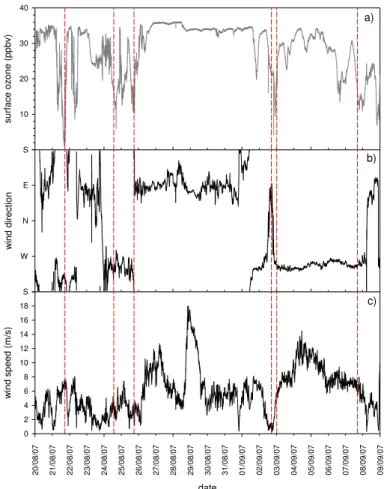
During the 2007 austral spring, six tethersonde flights were achieved, with surface air masses in each case approaching Halley from the west or south-west (see Fig. 2b), i.e. across the sea ice zone and/or Precious Bay. The wind speeds during each flight 5
ranged from 1 ms−1
to 7 ms−1
(see Fig. 2c), so all cases probed were relatively low wind speed ODEs. The timing of each flight relative to the condition of surface ozone is shown on Fig. 2a, and it is clear that launches were carried out during all stages of an ODE, i.e. during onset (24/8/07, 2/9/07 – flight a, 7/9/07), at totality (21/8/07), and during termination (25/8/07, 2/9/07 – flight b). The profiles of O3 and potential
10
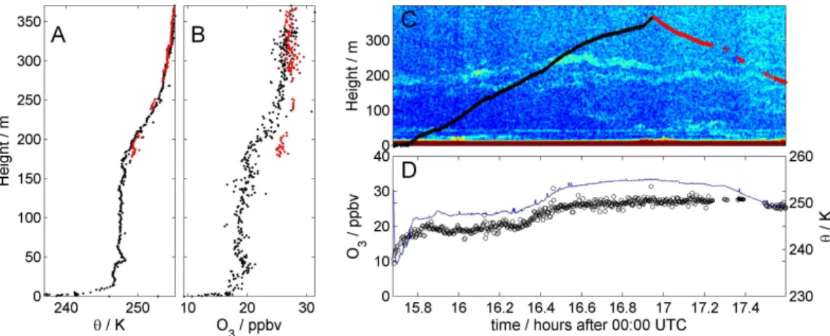
temperature measured during each experiment are shown in plots A and B of Figs. 3 to 8. Plot C of each figure shows the flight track of the tethersonde superimposed on the sodar trace to show the different air masses encountered by the sonde. Plot D shows the corresponding time-series of O3and potential temperature measured along
the flight track. Data were filtered according to battery voltage; once the voltage started 15
to drop, data were removed, so the amount of data recorded varies with each flight. As such data have not previously been assembled we examine them in some detail on a case by case basis.
ODEs are often referred to as boundary layer events, with the boundary layer top, or “inversion”, acting as the lid to the depletion. Indeed, an inversion is classically de-20
fined as the region of the boundary layer where the potential temperature gradient is positive. However, in polar regions, this becomes problematic. A key feature of polar regions is the persistent, deep, continually stratified lower atmosphere that is char-acterised by a positive temperature gradient throughout (Anderson and Neff, 2008). Within such a layer there is no inversion in the classical sense, and so no obvious 25
upper limit to the boundary layer based on temperature structure alone. For this rea-son, when presenting the tethersonde data we discuss atmospheric layering primarily in terms of the vertical potential temperature gradient, ∂θ
ACPD
10, 8189–8246, 2010Vertical structure of Antarctic tropospheric ozone
depletion events
A. E. Jones et al.
Title Page
Abstract Introduction
Conclusions References
Tables Figures
◭ ◮
◭ ◮
Back Close
Full Screen / Esc
Printer-friendly Version
Interactive Discussion height. The former gives an indication of atmospheric stratification, and the latter the
height to which mixing can be expected. To further assess degrees of mixing we cal-culate the Richardson number (Ri) when data quality allows. Ri is a measure of the balance between turbulence generation (by wind shear) and turbulence suppression by stratification (i.e. potential temperature gradient), and is defined as:
5
Ri=g
T
∂θ
∂z
∂U
∂z
2 (1)
whereU is the wind speed,gis the acceleration due to gravity (=9.81 ms−2
),T is am-bient temperature (K).Ri is thus a measure of stability (and hence degree of mixing) within an air mass; smallRi (large shear and small stratification) implies strong turbu-lence and hence strong vertical mixing; largeRi implies suppression or even absence 10
of turbulence, and hence low or zero mixing. A critical value ofRi =0.25 is often taken as a transition from one regime to the other (Stull, 1988). AsRi is based on gradients it is sensitive to measurement error, especially winds, and the relatively short sample time ofU at each level means theRi estimate will have error of up to 50%.
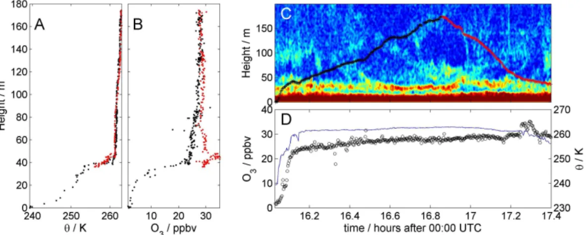
4.1.1 Profile experiment 21/8/07
15
During the flight of 21/8/07, ozone was almost completely depleted in a layer extending from ground level to∼30 m (Fig. 3b). This layer was characterised by a strong gradient
in potential temperature,∂θ
∂z, i.e. was highly stratified, andRi within this layer was
∼0.4, indicating intermittent or limited mixing. Between 30 m and 40 m there is a clear
discontinuity in both O3andθ, and above this discontinuity, little change in either O3or
20
θis visible up to the 175 m range of this flight. For the region from 40 m to 120 m, it is possible to calculateRi. Even though∂θ
ACPD
10, 8189–8246, 2010Vertical structure of Antarctic tropospheric ozone
depletion events
A. E. Jones et al.
Title Page
Abstract Introduction
Conclusions References
Tables Figures
◭ ◮
◭ ◮
Back Close
Full Screen / Esc
Printer-friendly Version
Interactive Discussion The sodar echogramme (Fig. 3c) shows little in the way of air mass structure above
40 m. Below 40 m, the echogramme shows a strong continual echo between 30 m and 40 m. Within the lowest 30 m there is evidence of residual structure, likely to arise from fossil convection (see Sect. 3.1.4).
The atmosphere thus appears to be split into two masses; a depleted layer extending 5
from the surface to ∼30 m and a layer above ∼40 m with background ozone mixing
ratios. Between is a transition region some 10 m deep.
During descent, no structure is evident in eitherθor O3until the sonde reaches the region of fossil convection (Figs. 3c and d), when small scale structure is again evident in both. The ozonesonde battery voltage dropped just after the instrument had once 10
again entered the transition region, so below this altitude data have been filtered out.
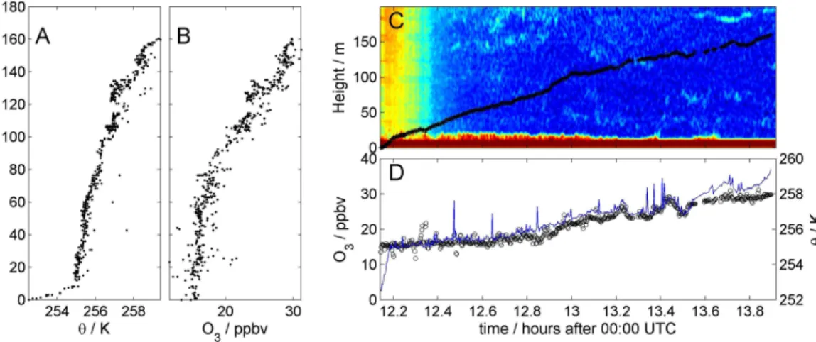
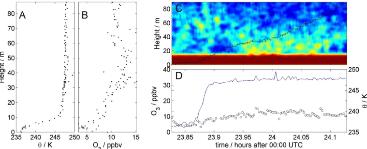
4.1.2 Profile experiment 24/8/07
During this flight, the ground-based surface ozone measurements (Fig. 2a) show that ozone was only partially depleted and that the ODE was still developing. The profile in potential temperature (Fig. 4a) shows a well-defined and extremely shallow layer 15
extending from the ground to ∼10 m height. This layer is also visible in the sodar
echogramme (Fig. 4c) which, after some initial wind noise, shows a shallow (∼20 m)
near-surface turbulent layer which decreases in height during the flight. Interestingly, there is no equivalent discontinuity in ozone visible from the sonde profile (Fig. 4b). Ac-cording to these data, ozone mixing ratios were depleted, but roughly constant from the 20
surface to a height of∼80 m, and above this altitude, mixing ratios gradually returned
to background amounts. The potential temperature data show that above the 10-m dis-continuity, the atmosphere is stratified throughout, and indeed, there is no turbulence signal on the sodar echogramme.
Our interpretation of these data is that a relatively warm air mass, already depleted 25
ACPD
10, 8189–8246, 2010Vertical structure of Antarctic tropospheric ozone
depletion events
A. E. Jones et al.
Title Page
Abstract Introduction
Conclusions References
Tables Figures
◭ ◮
◭ ◮
Back Close
Full Screen / Esc
Printer-friendly Version
Interactive Discussion depletion, however, was not affected, so the signals in ozone and potential temperature
are effectively decoupled.
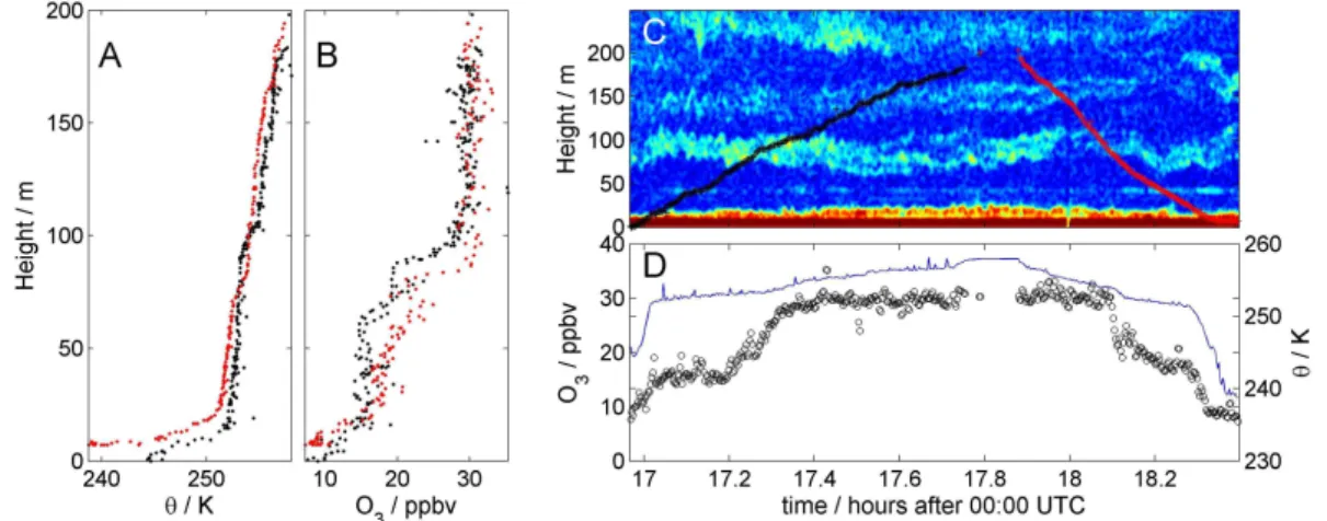
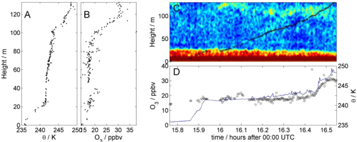
4.1.3 Profile experiment 25/8/07
The flight of 25/8/09 revealed more complex vertical profiles, with three distinct air masses probed. The greatest ozone depletion was evident in the well-defined and 5
highly-stratified layer that extended to∼20 m above the ground (Figs. 5a and b). The strongly positive∂θ
∂z indicates that heat was flowing from the atmosphere into the radiatively-cooling snow surface below. Ozone mixing ratios increased to between 15 and 20 ppbv in the region between ∼20 m and ∼80 m while ∂θ∂z, although small,
remained positive (indicating stratification). From∼80 m to∼100 m, a transition zone is
10
evident, characterised by an increase in stratification (∂θ
∂z=0.08 Km−1), and within which ozone mixing ratios increased rapidly. The sodar data (Fig. 5c) show a clear layer of increased turbulence within this region. Above 100 m, ozone mixing ratios reached, and remained at background amounts of roughly 30 ppbv to the top of the flight track at 200 m. On the descent flight, the∼100 m turbulent layer was still evident in the sodar
15
echogramme (Fig. 5c) and, according to the sharp discontinuity in ozone (Figs. 5a and d), was acting as a significant barrier to mixing.
We interpret these data as indicating three main air masses, with different histories that had been retained. Interestingly, in this example, a correlation between ozone and potential temperature is maintained in the lowest layer of the atmosphere.
20
4.1.4 Profile experiment 02/9/07 – daytime flight
The first flight on 2nd September was carried out mid-afternoon during the onset of an ODE. It revealed a series of layers in the atmosphere between the ground and the upper reaches of the sonde (see Fig. 6). The lowest was, once again, a well-defined and very shallow layer, reaching only∼15 m above the ground (Figs. 6a and b). Higher
25
ACPD
10, 8189–8246, 2010Vertical structure of Antarctic tropospheric ozone
depletion events
A. E. Jones et al.
Title Page
Abstract Introduction
Conclusions References
Tables Figures
◭ ◮
◭ ◮
Back Close
Full Screen / Esc
Printer-friendly Version
Interactive Discussion or no vertical gradient. The first spanned the region between∼60 m and 180 m, and
was characterised by ozone mixing ratios of∼20 ppbv and small potential temperature
gradient (<0.01 Km−1), i.e. neutrally stratified. The second extended above 250 m to the top of the profile (∼370 m), with ozone mixing ratios of ∼28 ppbv and ∂θ∂z =
0.02 Km−1. A region of mixing, with a clear gradient in both O
3 and θ, lay between
5
180 m and 250 m.
The surface winds on this occasion were light,∼2 ms−1, but the profile of wind speed,
and more significantly, wind direction (not shown) reveals that the two air masses were quite distinct. In the lower region, the air originated from the 270◦±20◦ sector (West),
while in the upper region, the air mass originated from 55◦±10◦ sector (North East).
10
Within the transition region, the winds drop to zero, and backs via North. In the lower region there is a local maximum in wind speed, (from near zero at the surface, and zero again in the transition region). Given the neutral stratification, the wind shear in this region should produce a well mixed air mass. In the upper region, the winds increase monotonically throughout, with∂U
∂z=0.033 s−1. This gives Ri =0.7, implying very 15
weak mixing.
The sodar data show two associated echo layers within the transition region, and we interpret these as the upper and lower limits of the shear region, where the air masses are sliding over each other. The clear difference in wind direction implies a different history for the air masses, the lower being recently advected over the ocean, the upper 20
being continental air (King 1989, 1993).
4.1.5 Profile experiment 02/09/07 – night-time flight
A second flight was carried out late on 2nd September which was only able to mea-sure to 85 m altitude. Above this height, the battery failed, probably because of the lower temperatures. It was dark during this flight, and, according to the surface ozone 25
ACPD
10, 8189–8246, 2010Vertical structure of Antarctic tropospheric ozone
depletion events
A. E. Jones et al.
Title Page
Abstract Introduction
Conclusions References
Tables Figures
◭ ◮
◭ ◮
Back Close
Full Screen / Esc
Printer-friendly Version
Interactive Discussion ground, but that, again, this structure was not reflected in the ozone profile (Fig. 7b).
During the dark, ozone-depletion chemistry would not be active, so a strong correlation betweenθand O3would not necessarily be expected.
4.1.6 Profile experiment 07/09/07
The final tethersonde flight of this campaign was carried out on 7th September during 5
daylight hours (Fig. 8). According to the surface ozone data (Fig. 2a), the air measured at Halley was only partially depleted, and the sonde was launched close to the maxi-mum depletion observed. Battery voltage was good to∼140 m on the ascent flight.
The flight shows three distinct atmospheric layers. A strong positive potential temper-ature gradient extends from the surface to∼20 m indicating highly stratified air (Fig. 8a).
10
This structure is not matched by structure in the ozone profile (Fig. 8b). These data suggest an air mass whose potential temperature structure is still evolvingen route to Halley, while ozone has not changed. Between 20 m and 100 m, the potential temper-ature gradient is much weaker, but nonetheless positive and therefore stratified. No significant change in ozone is measured over this distance. However, between 100 m 15
and 120 m, there is a transition zone with clear discontinuities in both ozone and po-tential temperature. Above∼120 m, ozone mixing ratios return to background amounts
(∼30 ppbv).
The sodar (Fig. 8c) shows associated echo return within the lowest 20 m, and again within the transition zone around 100 m altitude. Thus far, the event is similar to that 20
of the first flight on the 2nd of September (above), except in the amount of ozone de-pletion near the ground. Further similarity is observed in the winds, where, although not reversing in direction, the easterly component of the wind increases with height by 2 ms−1 within the transition zone, implying again maritime air advected underneath continental air. Further evidence is apparent in the sodar data, where fossil convec-25
ACPD
10, 8189–8246, 2010Vertical structure of Antarctic tropospheric ozone
depletion events
A. E. Jones et al.
Title Page
Abstract Introduction
Conclusions References
Tables Figures
◭ ◮
◭ ◮
Back Close
Full Screen / Esc
Printer-friendly Version
Interactive Discussion
4.1.7 Tethersonde study: implications
This was the first concentrated assessment of the detailed vertical structure of a num-ber of ozone depletion events. The overall technique used to study ODEs, using teth-ersonde launches triggered by surface ozone data, worked well, with a large number of ODEs probed and under a variety of stages of depletion. The tethersonde was able 5
to probe the lowest few hundred meters in great detail – a region of the atmosphere where free-flying sondes are essentially blind.
The tethersonde study revealed the enormous complexity within the lowest layers of the atmosphere and the influence exerted by atmospheric structure and dynamics on observed ozone profiles. The observations suggest that numerical modelling studies 10
aimed at reproducing ODEs observed at coastal sites will need to account in some detail for the influence of atmospheric dynamics on ozone mixing ratios. Such data would then provide excellent constraints against which to test ideas on local ozone depletion processes. It is also clear that the lowest atmospheric layer at Halley can be extremely shallow at times, something that is more closely associated with sites on the 15
Antarctic plateau.
The data, further, highlight the difficulty in defining a relevant boundary layer height. This issue is important, for example, when translating a measured surface flux into a boundary layer concentration, and also when deriving a mixing ratio from a slant or vertical column density. Assessment of mixing height would therefore seem a wel-20
come companion to many chemical measurement programmes. Further, considerable variability can exist in the profile of ozone, and it appears that concentrations can be influenced by several physical layers at different heights. For example, a significantly lower mixing height can be rapidly established as air moves from over the convective sea ice zone (mixing height of the order 100 m) to over the stably stratified ice shelf 25
(mixing height∼20 m). We note also that the relationship between ozone and potential
ACPD
10, 8189–8246, 2010Vertical structure of Antarctic tropospheric ozone
depletion events
A. E. Jones et al.
Title Page
Abstract Introduction
Conclusions References
Tables Figures
◭ ◮
◭ ◮
Back Close
Full Screen / Esc
Printer-friendly Version
Interactive Discussion Finally, as the blimp profiling system cannot be deployed under windy conditions,
the low altitude profiles reported here are, by definition, all relatively low wind speed events (∼1 ms−1 to ∼7 ms−1). Low wind speed ODEs are often associated with local
depletion (e.g. Simpson et al., 2007), and indeed two local ODEs previously studied at Halley were measured at wind speeds between zero and ∼5 ms−1 (Jones et al.,
5
2006). The majority of the tethersonde profiles reported here appear to arise from local processing under quiescent conditions, and it is interesting to note that the ozone depletion is restricted to the lowest 10s to ∼100 m altitude. Maps of BrO measured
by the satellite-borne SCIAMACHY (SCanning Imaging Absorption SpectroMeter for Atmospheric CHartographY) instrument (Richter et al., 1998; Bovensmann et al., 1999) 10
(not shown), indicate no major increases in the BrO column in the Halley region during the ODEs measured by the tethersonde. This may be linked to the low sun at the time of satellite overpass over Halley at this time of the year but alternatively may imply that on these occasions the local production of bromine compounds was not sufficient to significantly enhance the BrO column. In terms of export of halogens 15
or of air low in ozone that might affect the radiative balance of the atmosphere, it therefore appears that low wind speed ODEs, driven by local processing, have few wider atmospheric implications. Their merit, however, lies in their providing excellent cases against which to test kinetics and chemical mechanisms involved in depleting polar tropospheric ozone.
20
4.2 The 1987 free-flying ozonesonde study
4.2.1 Time-series of ozone profiles
Data from the free-flying ozonesonde study show considerably less fine-scale detail than the tethersonde profiles described above, but enable a much broader view to be gained of ozone behaviour throughout the troposphere. Figure 9 is a contour plot 25
ACPD
10, 8189–8246, 2010Vertical structure of Antarctic tropospheric ozone
depletion events
A. E. Jones et al.
Title Page
Abstract Introduction
Conclusions References
Tables Figures
◭ ◮
◭ ◮
Back Close
Full Screen / Esc
Printer-friendly Version
Interactive Discussion the data coverage, the degree of smoothing in the diagram and the days when no sonde
launches were made. The lack of at least daily data coverage becomes problematic later, when trying to understand mechanisms driving high altitude ozone depletion by linking with meteorological information available at 6-hourly resolution. The reason for the lack of sonde launch varies – sometimes due to the planned schedule, but 5
sometimes due to high wind speeds, a fact which becomes relevant later.
There are various features in Fig. 9 that are immediately obvious. Firstly, the data coverage varies quite considerably during this period shown. For example, from 25th August to 6th September, sondes were launched every day. In contrast, from 7th September to 15th September there were only 3 sonde launches. Also obvious are 10
the ODEs, indicated by the blues of the false colour scale, which were measured be-tween 22nd August and 7th October. The vertical extent of the ODEs varies consid-erably. There are various occasions when depletion extends only to a few hundred meters above the ground (e.g. 25th/26th August and 7th October). However, there are also profiles showing ozone depletion to several kilometres altitude, to a maximum of 15
∼3.5 km on both 29th September and 3rd October. Of note also are two dislocated
events, where ozone at ground level shows unperturbed background concentrations, but by an altitude of roughly 200 m, significant depletion is apparent. Such ODEs are by definition, transparent to surface ozone measurements, and are an example that the ground-based record does not reveal the complete picture regarding ODEs. Studies 20
aimed at addressing trends in ODEs would need to take that into account.
The data thus hold significant amounts of information, but, as the record is somewhat limited by periods when no sondes were launched, they must be interpreted with care. For example, a severe ODE is evident on 22nd August with less extensive depletion apparent on 25th and 26th August. However, as there were no sonde launches on 25
ACPD
10, 8189–8246, 2010Vertical structure of Antarctic tropospheric ozone
depletion events
A. E. Jones et al.
Title Page
Abstract Introduction
Conclusions References
Tables Figures
◭ ◮
◭ ◮
Back Close
Full Screen / Esc
Printer-friendly Version
Interactive Discussion They can nevertheless considerably extend our understanding of ODEs that occur
at Halley. For example, a key question that can be addressed with these data is: what drives ODEs to such remarkable altitudes? Given that the depletion of ozone is caused by a source associated with sea ice, i.e. initially ground-based, how can the signature of depletion attain heights to several kilometres above the ground? We explore this 5
issue in the rest of this paper, focussing on events where ozone depletion was evident in the profile up to and above 1 km altitude. We initially consider the air mass origin of dislocated events using 5-day back trajectories. We then consider profiles where depletion is continuous upwards from ground level, and the regional meteorological situation around the time of the profile measurements.
10
4.2.2 Origin of the dislocated events
Back trajectories were calculated for both of the dislocated events using the on-line trajectory service of the British Atmospheric Data Centre (www.badc.rl.ac.uk). The tra-jectories were calculated at a resolution of 2.5◦, the maximum available for this time period, and were run backwards from Halley for 5 days. In each case trajectories end-15
ing at different pressure levels were calculated in order to provide information on the history of air mass at different heights in the ozone profile.
Figures 10a and b shown the histories of air arriving over Halley on 21st and 28th September. On each occasion, air at ground level shows unperturbed concentrations of ozone while those at altitude show significant depletion. The back trajectories show 20
that in both cases, air arriving close to ground level (980 and 950 hPa) had originated over the cold continent to the east of Halley. Air arriving at higher altitudes, shown by the sonde data to be depleted in ozone, had tracked over the sea ice zone. On 21st September the route was over the frozen southern Weddell Sea with an approach to Halley from the south west. On 28th September, air had originated much further north, 25
ACPD
10, 8189–8246, 2010Vertical structure of Antarctic tropospheric ozone
depletion events
A. E. Jones et al.
Title Page
Abstract Introduction
Conclusions References
Tables Figures
◭ ◮
◭ ◮
Back Close
Full Screen / Esc
Printer-friendly Version
Interactive Discussion (not shown) reveals, in both cases, an increase in moisture in the ozone-depleted layer.
The fact that the profile at Halley was dislocated thus appears to be driven simply by different large-scale air mass origins. This conclusion is in line with observations re-ported by Wessel et al. (1998) where an ozonesonde launched at Neumayer station (8◦W, 70◦S) revealed air with limited ozone depletion at ground level that was overlain 5
by a highly depleted air mass. Wessel et al. explained their observation as cold kata-batic surface winds, originating over the continental ice shelf, lifting up warmer and less dense marine air masses that had lower ozone mixing ratios. We return to this later.
4.2.3 The broader picture
To further explore the drivers of high altitude ODEs we consider charts of mean sea 10
level pressure (mslp), together with 10-m wind vectors, to gauge the regional mete-orological situation around the time of the observed ODEs. We utilise the European Centre for Medium Range Weather Forecasts (ECMWF) 40-year reanalysis (ERA-40), which is described in Uppala et al. (2005). The reanalysis has been retrieved on a Gaussian N80 grid, with a grid cell spacing of∼125 km.
15
In the relevant plots the 10-m wind speed vectors are classified by a series of colours according to their speed. The thresholds were chosen according to a study on an Antarctic ice shelf (Mann et al., 2000) which concluded that when the 10-m wind speed reached between 8 ms−1and 12 ms−1(shown in amber on the plots) particles of snow or ice were dislodged from the snow surface and bounced into a∼10 cm deep
“salta-20
tion layer”. At 10-m wind speeds in excess of 12 ms−1 (shown in red on the plots) particles were lofted out of the saltation layer and formed what is classically referred to as blowing snow. ERA-40 wind vectors are likely to give a good indication of wind speed, and therefore reflect whether snow was lofted or blowing.
Figure 11a shows the profile of ozone as measured using the free-flying balloon-25
ACPD
10, 8189–8246, 2010Vertical structure of Antarctic tropospheric ozone
depletion events
A. E. Jones et al.
Title Page
Abstract Introduction
Conclusions References
Tables Figures
◭ ◮
◭ ◮
Back Close
Full Screen / Esc
Printer-friendly Version
Interactive Discussion with a huge low pressure system situated off-shore of Halley and encompassing the
majority of the Weddell Sea area. The 10-m wind vectors on 21/8/87 are shown in Fig. 11c and their colouring shows that over large areas, snow/ice will be lofted either into a saltation layer or higher into the atmosphere as blowing snow. Unfortunately no sonde was launched from Halley on 21/8/87 precisely because of the high winds. By 5
22/8/87, ERA-40 charts show that the depression is still present over the Weddell Sea, but that it is much less intense than on the 21st.
Figure 12a shows the ozone profile on 21st September 1987, the first dislocated event for which we calculated trajectories, above. Again a typical un-depleted profile from the middle of the month is also shown, and it is clear that on 21/9/87, ozone is 10
depleted to∼2000 m, but with the largest bite from the profile extending from∼200 m to ∼1000 m. The back trajectories in Fig. 10a show that the air originating within the most
depleted layer arrived at Halley from over the southern Weddell Sea. Figure 12b shows the mslp on this day, and the presence of a large, moderately deep low pressure system over the Weddell Sea. Figure 12c shows that the wind speeds at 10-m maximise in the 15
8 ms−1to 12 ms−1range, suggesting that snow and ice would be lofted into a saltation layer. The air, shown by the back trajectory analysis to arrive at altitudes over Halley of between 900 and 800 hPa, with its route across the southern Weddell Sea, is thus highly likely to have been impacted by the depression. The following day the winds were too high to launch a sonde, so we have no information on whether depletion was 20
sustained.
The ozonesonde launched on 24th September 1987 shows small but limited amounts of depletion in the ozone profile (not shown). That launched on 25th Septem-ber 1987, in contrast, shows clear and significant depletion in the ozone profile to over 2000 m altitude (see Fig. 13a). From the mean sea level plot of the 24/9/87 (Fig. 13b), 25
ACPD
10, 8189–8246, 2010Vertical structure of Antarctic tropospheric ozone
depletion events
A. E. Jones et al.
Title Page
Abstract Introduction
Conclusions References
Tables Figures
◭ ◮
◭ ◮
Back Close
Full Screen / Esc
Printer-friendly Version
Interactive Discussion storm, but no response was evident at that time in the Halley profile. On 25th
Septem-ber 1987, it is clear from the ERA-40 data (not shown) that the depression, although still present, was considerably weaker than on the 24th. By the 26th September 1987, although depletion is still evident in the ozone profile (Fig. 14a), the centre of the de-pression had shifted northwards (Fig. 14b) and the wind speeds across the Weddell 5
Sea had eased considerably (Fig. 14c). It is likely that the depletion evident on the 26th was a remnant of earlier ozone destruction.
Figure 15a shows the ozone profile measured on 28th September, the second dislo-cated event described above. The back trajectory calculation (Fig. 10b) shows that air in the layer between 900 and 700 hPa (∼3000 m) had passed over the sea ice zone to
10
the north west of Halley before arriving over the base. The mean sea level plot for 27th September 1987 (Fig. 15b) shows that a large low pressure system was present in this area on the day before the depleted profile was measured at Halley. The 10-m wind speed vectors suggest that the depression resulted in considerable amounts of blowing or saltating snow in the atmosphere (Fig. 15c). Similar to the event described above, 15
mslp and 10-m wind vector charts (not shown) indicate that on 28th September, the low was still present although weaker, but with wind speeds still sufficient to cause sus-pended snow. By 29th September, the depression influencing Halley had completely dissipated (Fig. 16b) such that the winds in the vicinity of Halley had eased (Fig. 16c) – a new low pressure system had formed in the western Weddell Sea area but with 20
no influence on air masses at Halley at that time. The ozonesonde released at Halley on September 29th shows that ozone depletion extended from the surface to well over 3000 m altitude (Fig. 16a) most likely a remnant of processing over the previous days.
The final sonde launch of 1987 that showed ozone depletion at considerable altitudes was that of 3rd October. The sonde was launched around 1600, and Fig. 17a) shows 25
that depletion was evident from the surface to∼2500 m, with a maximum around 800 m
ACPD
10, 8189–8246, 2010Vertical structure of Antarctic tropospheric ozone
depletion events
A. E. Jones et al.
Title Page
Abstract Introduction
Conclusions References
Tables Figures
◭ ◮
◭ ◮
Back Close
Full Screen / Esc
Printer-friendly Version
Interactive Discussion vectors (Fig. 17c) suggest that the atmosphere would have been influenced by lofted
and blowing snow in the Halley region around 0600. No significant depletion is evident in the ozonesonde launch of 2nd October. These data help to provide some time constraints for ozone processing and suggest that significant depletion can occur within 10 h of the low pressure maximum.
5
4.2.4 Free-flying ozonesonde study at Halley: conclusions
In a recent paper we derived a relationship describing the likelihood of ODEs based upon wind speed (see Jones et al., 2009, Fig. 12d). The pre-requisite of low wind speeds and a stable boundary layer has been described by a number of authors (e.g. Jacobi et al., 2006; Jones et al., 2006; Simpson et al., 2007). In addition, Jones 10
et al. (2009) demonstrated that ODEs can develop under conditions of high winds and blowing snow. The conclusion was arrived at from a detailed case study around Hal-ley and the Weddell Sea in which an active ODE appeared to be generated during an intense Antarctic storm. Ground-based measurements at Halley showed that during the storm, saline blowing snow was lofted into the atmosphere. Concurrent satellite 15
data revealed an extensive region of enhanced BrO across the Weddell Sea. These observations added considerable support to a 3-D modelling study of Yang et al. (2008) which suggested that blowing snow events over sea ice could be a major source of sea salt aerosol, and that this aerosol could in turn generate bromine that would destroy tropospheric ozone. No information about the vertical profile of ozone was available for 20
the Halley case study.
Windy conditions in themselves are of course not sufficient to drive ozone deple-tion, and the 1987 observations clearly demonstrate this point. For example, on 24th September 1987, a large and vigorous low pressure system was operative across the Weddell Sea, with lofted and blowing snow likely present in the region of Halley. How-25
ACPD
10, 8189–8246, 2010Vertical structure of Antarctic tropospheric ozone
depletion events
A. E. Jones et al.
Title Page
Abstract Introduction
Conclusions References
Tables Figures
◭ ◮
◭ ◮
Back Close
Full Screen / Esc
Printer-friendly Version
Interactive Discussion that temperatures across the Weddell Sea were significantly higher on 24th September
than on the following day when ozone depletion was observed to over 2 km.
So, although windy conditions in themselves are not enough, the reverse appears to be true – it is clear from the data presented here that all the 1987 events with high alti-tude ozone loss were associated with significant atmospheric depressions, windy con-5
ditions, and lofted or blowing snow. In each case, the low pressure system preceded the measurement of the depleted profile, but unfortunately the temporal resolution of the data is too limited to allow a clear statement on the timescales involved in process-ing and depletion which might be used to test/confirm the mechanisms proposed by Yang et al. (2008).
10
5 Discussion
5.1 Re-visiting earlier published studies
Although the analyses from 1987 Halley are very consistent, these are a limited number of events measured at a single location. In order to expand our dataset, we consider here published ozone soundings made at other Antarctic stations that also show high 15
altitude ozone loss. To gain the broader picture, we again turn to ECMWF re-analyses. For the period up to 2001 we utilise the ERA-40 reanalysis (described earlier), and for more recent data we analyse the ECMWF Interim Reanalysis, which starts in 1989 and is updated to the present time. The latter has also been retrieved on a Gaussian N80 grid, with a grid cell spacing of∼125 km.
20
Wessel et al. (1998) focussed on dynamical processes occuring during ODEs ob-served at Neumayer station in austral spring 1993. They highlighted three dislocated events, the most intense featuring depletion to∼3000 m altitude. From back-trajectory
calculations, they concluded that the dislocation arose because air low in ozone, with a source over the sunlit sea ice, was uplifted over continental air. They further noted 25
ACPD
10, 8189–8246, 2010Vertical structure of Antarctic tropospheric ozone
depletion events
A. E. Jones et al.
Title Page
Abstract Introduction
Conclusions References
Tables Figures
◭ ◮
◭ ◮
Back Close
Full Screen / Esc
Printer-friendly Version
Interactive Discussion developed over the ice-covered South Atlantic Ocean. Although the discussion was
in terms of transport, rather than as a key player in the depletion process, a clear link was nonetheless made between high altitude ODEs and low pressure systems.
A paper by Kreher et al. (1997) presents a number of ozone profiles, and extends the picture by including halogen data. They describe measurements of BrO made in 5
austral spring 1995 at Arrival Heights, part of the New Zealand station on the edge of the Ross Sea (77.8◦S, 166.7◦E). The observations were made with a zenith sky DOAS (Differential Optical Absorption Spectrometer) at high solar zenith angle (86◦ and 90◦) – i.e. twilight dawn and dusk. In particular, they focus on two events with enhancement in tropospheric BrO, the first from dusk on 24th to dusk on 26th August and the second 10
from dusk on 15th to dusk on 16th September. The authors link their BrO data with ozonesonde measurements made at the nearby McMurdo station on 25th August and 15th September, which show depletion in the profile to several kilometres altitude. We studied the ERA-40 meteorological charts for that region and time period, and found that on 23rd August, the day before enhanced BrO was observed, a low pressure 15
system was situated in the area which by noon was over the Ross Sea. By 1800, its position was such that, as well as enhancing katabatics descending from the Antarctic Plateau, it was drawing air from the sea ice zone to Arrival Heights (see Fig. 18a). Wind speeds were sufficiently high to cause saltation and blowing snow (Fig. 18a). The storm lasted through the night but ERA-40 charts show that it eased over the following 20
day, such that by 1800 on 24th, 10-m wind speeds around Arrival Heights were below the threshold for lofted snow. A similar situation arose around the time of the second enhanced BrO event. An atmospheric depression, centred over the boundary between the Ross Ice Shelf and the Ross Sea on 14th September resulted in high wind speeds in the region around Arrival Heights and generally high winds across the whole area 25
ACPD
10, 8189–8246, 2010Vertical structure of Antarctic tropospheric ozone
depletion events
A. E. Jones et al.
Title Page
Abstract Introduction
Conclusions References
Tables Figures
◭ ◮
◭ ◮
Back Close
Full Screen / Esc
Printer-friendly Version
Interactive Discussion A subsequent paper by Roscoe et al. (2001) used the results of Kreher et al. (1997)
and expanded them to include some additional data from Neumayer. Specifically, the authors considered zenith sky DOAS and ozonesonde measurements from Neumayer that showed enhanced tropospheric BrO on 2nd August 1995 that coincided with an ozone profile that was severely depleted to∼3 km altitude. ERA-40 charts show that
5
on 1st August 1995, a moderate depression was situated offshore of Neumayer, with winds in the coastal region above the threshold for saltating and blowing snow (see Fig. 18c). By 2nd August, this low pressure system had eased considerably, although, according to ERA-40 charts (not shown), wind speeds were still sufficient to loft snow into a saltation layer. No ozone sonde was launched on 1st August, so we have no 10
way of knowing the state of the ozone profile during the windier preceding day. Again, however, a high altitude ODE and enhanced BrO were associated with an atmospheric low pressure system.
In a more recent paper, Frieß et al. (2004) focused on measurements made at Neu-mayer station in austral spring 1999 and 2000. Their data set included zenith sky DOAS 15
observations of BrO as well as ozone soundings and they interpreted their results in the context of duration of sea ice contact. From their data they derived a meteorological scenario to describe conditions responsible for depletion in the ozone profile, in which an air mass located over the sea ice is driven south towards the station by an eastward moving depression. They further note that air masses from the sea ice are transported 20
to altitudes of∼4000 m by advection processes caused by cyclonic activity above the
ice covered ocean. We discuss the Frieß et al. paper further below.
Thus, in all previous studies of Antarctic ozone profiles, there is either a stated link to low pressure systems, or a link that can be derived by some additional analysis (using the ERA-40 charts). There are also the first hints of a link between low pressure 25
ACPD
10, 8189–8246, 2010Vertical structure of Antarctic tropospheric ozone
depletion events
A. E. Jones et al.
Title Page
Abstract Introduction
Conclusions References
Tables Figures
◭ ◮
◭ ◮
Back Close
Full Screen / Esc
Printer-friendly Version
Interactive Discussion
5.2 Expanding the low pressure system/BrO link
The papers by Jones et al., (2009) and Yang et al., (2008) described above raise the idea that atmospheric low pressure systems with sufficient wind speeds to loft saline blowing snow can be a source of bromine to the atmosphere with the potential to deplete tropospheric ozone. Considerable evidence to support this idea can be 5
found within earlier publications. For example, Kreher et al. (1997) note that the initial phase of both BrO events they observed coincided with high surface winds and blowing snow. Frieß et al. (2004) note that most periods of elevated BrO were accompanied by strong enhancement in O4absorption, a diagnostic for tropospheric light path. The authors suggest that this may have been due to sea salt particles, but also state that 10
snow drift could provide the scattering particles.
Importantly, satellite observations of BrO are available from the GOME (Global Ozone Monitoring Experiment) instrument (Richter et al., 1998; Burrows et al., 1999) from 1996 to 2004, so are available for the period of measurements reported by Frieß et al. (2004). Indeed maps of BrO are presented for a number of days to support the 15
zenith sky DOAS observations reported in the paper. We are thus able to combine, for some days, observations of surface ozone, the ozone profile, BrO from both ground-based zenith sky DOAS and satellite-borne imaging, together with ERA-40 charts of regional meteorology. The satellite maps show total column BrO, so do not separate troposphere and stratosphere, but provide a qualitative indication of BrO enhancement. 20
We refer to data published by Frieß et al. where it exists, and supplement with other sources where necessary. We focus on the three days from the Frieß et al. paper that show the most severe depletion in the surface ozone record. Firstly, on 9th September 1999, Frieß et al. show that measured surface ozone was∼5 ppbv; the ozonesonde
launched that day shows that the depletion extended to roughly 1.5 km altitude; the 25
ACPD
10, 8189–8246, 2010Vertical structure of Antarctic tropospheric ozone
depletion events
A. E. Jones et al.
Title Page
Abstract Introduction
Conclusions References
Tables Figures
◭ ◮
◭ ◮
Back Close
Full Screen / Esc
Printer-friendly Version
Interactive Discussion over the Weddell Sea, with wind speeds in excess of 12 ms−1, that is co-located with a
cloud of enhanced BrO.
Equally severe depletion is evident in the surface ozone record for 11th Septem-ber 1999, and again, BrO observed by the DOAS is enhanced. No ozone pro-file data is presented in the Frieß et al. paper for this day, but the propro-file is 5
available from the Neumayer web service (http://www.awi.de/en/infrastructure/ stations/neumayer station/observatories/meteorological observatory/data access/ upper air soundings/full vertical resolution/) (K ¨onig-Langlo, 2007a). Ozone depletion (not shown) is clear to roughly 3 km altitude. The GOME map for 11th September 1999 (Fig. 19b) shows an extensive cloud of BrO to the north of Neumayer, which, according 10
to the ERA-40 charts of mslp and 10-m wind vectors (Fig. 19b), again coincides with a vigorous atmospheric low pressure system.
On 23rd September 2000, the third example, Frieß et al. show that surface ozone is depleted to∼5 ppbv, while BrO is enhanced. They further present GOME BrO showing
a “hotspot” offshore of Neumayer. The ozone profile, again from the Neumayer web 15
service (K ¨onig-Langlo, 2007b), shows that ozone depletion extended to roughly 2 km altitude, and the ERA-40 charts show a low pressure system offshore of Neumayer (see Fig. 19c). This case raises the issue of timing, as the low pressure system of 23rd September is the residual of a more vigorous system that was influencing the Neumayer region over the previous two days.
20
The maps and charts presented in Fig. 19 also show other occasions of coincident low pressure systems and enhanced BrO. These are particularly evident around the Ross Sea, with a very clear example being the BrO hot spot and low pressure system on 23rd September (Fig. 19c).
It thus appears from this ensemble of data and analyses that high altitude ozone 25
ACPD
10, 8189–8246, 2010Vertical structure of Antarctic tropospheric ozone
depletion events
A. E. Jones et al.
Title Page
Abstract Introduction
Conclusions References
Tables Figures
◭ ◮
◭ ◮
Back Close
Full Screen / Esc
Printer-friendly Version
Interactive Discussion
5.3 Why atmospheric low pressure systems?
Satellite imagery and high resolution meteorological analyses reveal that there is a spectrum of atmospheric low pressure systems in high southern latitudes from the mesoscale (less than 1000 km horizontal resolution) “polar lows” to synoptic-scale de-pressions with a diameter of 2000 to 3000 km. Polar lows tend to have a lifetime of 5
less than 24 h, but they can be very vigorous with winds in excess of gale force (Ras-mussen and Turner, 2003). The synoptic-scale lows usually have a lifetime of several days, although the detailed structure of the systems can change considerably during its evolution.
On satellite imagery most depressions are characterised by having the cloud or-10
ganised into comma-shaped or spiraliform bands, which often define the boundaries between air masses. The imagery also shows that many polar lows develop in the southerly air flow to the west of a large depression during cold air outbreaks.
By definition, all low pressure systems are associated with low level convergence and general ascent, with divergence at upper levels. However, the cloud bands indicate 15
areas of particularly marked ascent, and models and radar data have shown that the air flow in these areas consists of a number of “conveyor belts”, streams of rapid advection with slope, and not just simple ascent up a frontal surface. A warm conveyor takes air from the surface to the upper levels of the cyclonic system, the air being replaced by the descending cold air. Larger depressions can have ascent from the surface to the 20
upper troposphere.
Polar depressions thus provide the conditions for high wind speeds, and thereby blowing snow, at ground level, and a mechanism to transport processed air to consid-erable altitudes.
While blowing snow appears to contribute to the mechanism for ODEs at high wind 25